Three-dimensional inversion of magnetotelluric impedance tensor data and full distortion matrix

Geophysical Journal International

Geophys. J. Int.(2015)202,464–481 doi: 10.1093/gji/ggv144

GJI Geomagnetism, rock magnetism and palaeomagnetism

Three-dimensional inversion of magnetotelluric impedance tensor data and full distortion matrix

A. Avdeeva,

M. Moorkamp,

D. Avdeev,

M. Jegen

and M. Miensopust

1GEOMAR, Wischhofstrasse1-3, D-24148Kiel, Germany. E-mail:aavdeeva@geomar.de

2Department of Geology, University of Leicester, University Road, Leicester, LE1 7RH, United Kingdom

3Institute of Terrestrial Magnetism, Ionosphere and Radiowave Propagation, Russian Academy of Sciences,142190, Troitsk, Moscow Region, Russia

4Dublin Institute for Advanced Studies,5Merrion Square, Dublin2, Ireland

Accepted 2015 March 30. Received 2015 March 28; in original form 2014 May 7

S U M M A R Y

Galvanic distortion of magnetotelluric (MT) data due to small-scale surficial bodies or due to topography is one of the major factors that prevents accurate imaging of the subsurface. We present a 3-D algorithm for joint inversion of MT impedance tensor data and a frequency- independent full distortion matrix that circumvents this problem. We perform several tests of our algorithm on synthetic data affected by different amounts of distortion. These tests show that joint inversion leads to a better conductivity model compared to the inversion of the MT impedance tensor without any correction for distortion effects. For highly distorted data, inversion without any distortion correction results in strong artefacts and we cannot fit the data to the specified noise level. When the distortion is reduced, we can fit the data to an RMS of one, but still observe artefacts in the shallow part of the model. In contrast, in both cases our joint inversion can fit the data within the assumed noise level and the resulting models are comparable to the inversion of undistorted data. In addition, we show that the elements of the full distortion matrix can be well resolved by our algorithm. Finally, when inverting undistorted data, including the distortion matrix in the inversion only results in a minor loss of resolution. We therefore consider our new approach a promising tool for the general analysis of field MT data.

Key words: Inverse theory; Electromagnetic theory; Magnetotellurics.

1 I N T R O D U C T I O N

One problem that has prevented the wider use of magnetotelluric (MT) data in the geophysical community is the influence of gal- vanic distortion. This term describes the distortion of the measured electric fields at all frequencies by small-scale inhomogeneities due to charge accumulation at the boundaries (Berdichevskiy &

Dmitriev1976). As a consequence the observed MT impedances Z^obs(ω), which are transfer functions between electric and magnetic fields are also distorted at all frequenciesω. This distortion can be described by multiplying the complex regional impedance ten- sorZ(ω) by a frequency independent real valued distortion matrix C=

Cx x Cx y

CyxCyy

, viz.

Z^obs(ω)=CZ(ω)=

Cx xZx x+Cx yZyx Cx xZx y+Cx yZyy

CyxZx x+CyyZyx CyxZx y+CyyZyy

.

(1)

∗Now at: Leibniz Institute for Applied Geophysics, Stilleweg 2, D-30655 Hannover, Germany.

Galvanic distortion can be caused by any inhomogeneities which are smaller than the inductive scale length of the highest considered frequency. As long as we include these inhomogeneities in our modelling and inversion, the effect will be correctly considered when analysing the data. However, in the most extreme case the inhomogeneities can be on the order of centimetres and therefore will be inaccessible to precise physical modelling for the foreseeable future.

For 1-D and 2-D structures, a large number of techniques exist to deal with or to remove galvanic distortion of MT data. Good overviews of these methods can be found in Jiracek (1990), Groom

& Bahr (1992) and Jones (2011). In a 1-D environment we can determine the distortion matrixCup to one unknown scale factor (Bibbyet al.2005; Weidelt & Chave2012) and in a 2-D environment we can determine Capart from two unknown scale factors (e.g.

Groom & Bailey 1989; Bibbyet al. 2005). In both cases these scale factors shift the apparent resistivities at all frequencies by an unknown amount and they are therefore termed static shifts.

Mathematically this is equivalent to factoring the distortion matrix into a determinable part C^det multiplied with an indeterminable diagonal matrixS=

S1 0 0 S₂

, and in 1-D we haveS1=S2. Once 464 ^CThe Authors 2015. Published by Oxford University Press on behalf of The Royal Astronomical Society.

3-D MT inversion of distorted data 465 we have considered the effect ofC^det, for example through Groom-

Bailey decomposition (Groom & Bailey1989), the unknown matrix Sonly affects the apparent resistivities, but not the phases.

For 3-D structures the problems caused by galvanic distortion become more complex, as we now cannot make simplifying as- sumptions about the form ofC(see Bibbyet al.2005, for more details). The unknown elements ofCnot only shift the apparent re- sistivities, but the elements ofZ^obsare now mixtures of the elements ofZ(see eq. 1). This means that in a general 3-D environment, not only the apparent resistivities, but also the phases, are different compared to the undistorted impedances (see also Fig.2below).

Thus, 3-D inversion of distorted data requires new approaches.

Patro & Egbert (2011) and Kelbertet al.(2012) allow the 3-D in- version to put conductive and resistive small scale anomalies at the surface layers to compensate for distortion effects. Sasaki & Meju (2006) jointly invert for resistivity structure and static shift. They test their inversion on various synthetic data and obtain encourag- ing results. However, Jones (2011) points out that the simplifying assumption of static shift, that is assuming that the matrixChas diagonal form, might not be appropriate for 3-D structures.

When high frequency (>10 Hz) MT data are acquired, it is pos- sible to determine static shifts from central-loop transient electro- magnetic (TEM) soundings performed at the same locations as the MT measurements. ´Arnasonet al.(2010) describe a procedure to incorporate static shifts determined from coincident MT and TEM into 3-D MT inversion. However, they also assume a diagonal form ofCand therefore the comment of Jones (2011) applies in a similar way as it does for Sasaki & Meju (2006).

Patro et al.(2013) take a different approach to circumventing problems with galvanic distortion. They invert MT phase tensor data (Caldwellet al.2004) which is not affected by galvanic distortion.

They show encouraging results for both synthetic and real data, but also report that the quality of their inversion results is much more sensitive to the starting model than with full tensor MT data. From a theoretical perspective it is plausible that reducing the number of data by a factor of two results in a loss of resolution. However, no detailed resolution analysis for phase tensor inversion has been published, yet.

A combination of the approach by ´Arnasonet al. (2010) and the phase tensor analysis of Bibbyet al.(2005) is used by Heise et al.(2008) to invert data from the Taupo Volcanic Zone. Where the phase tensor analysis of their high-frequency data indicate a 1-D Earth, they determine Cup to an unknown scale factor and then use TEM soundings to determine that factor. Where the phase tensor analysis does not indicate a 1-D situation, they determine an approximate resistivity and revert to a diagonal form ofCto correct their data before inversion.

In this paper, we propose a similar approach to Sasaki & Meju (2006), but we include the frequency-independent elements of the full distortion matrix C, rather than static shifts, as additional parameters into our 3-D inversion. It should be noted that de Groot-Hedlin (1995) and Ogawa & Uchida (1996) presented a sim- ilar approach for 2-D inversion, and Miensopust (2010) describes an analogous strategy to deal with galvanic effects in her 3-D inver- sion code, but does not show any tests of the distortion aspects of her code.

We test our inversion on several distorted synthetic data sets generated from a benchmark model with a range of near-surface structures. We show that the joint inversion of MT impedance tensor data and full distortion matrix can very well recover the elements of the distortion matrix and obtain a resistivity model similar to the

true model. Furthermore, it is possible to fit the distorted data to an RMS value of one regardless of the amount of distortion when the joint inversion strategy is used. For an inversion of the MT impedance tensor alone, it is impossible to fit the highly distorted data to a desirable value of RMS and the inversion result contains many strong artefacts. When the distortion is relatively small we can fit the data within the assumed noise, but still observe significant artefacts in the near surface layers.

2 I N V E R S I O N M E T H O D

Our inversion is based on the 3-D MT inversion codex3Diand de- tails about the method are described in Avdeev & Avdeeva (2009) and Avdeevaet al. (2012). It employs a limited-memory quasi- Newton optimization method to minimize a Tikhonov-type regular- ized objective functionϕ. Our objective function is a weighted sum of three parts, the data misfitϕd(σ,C), the smoothness constraint ϕs(σ), and a constraint on the amount of galvanic distortionψ(C), viz.

ϕ(σ,C, λ, ν)=ϕd(σ,C)+λϕs(σ)+νψ(C)−→

σ,C min. (2) The parametersλandνare trade-off parameters. For largeλwe do not allow strong spatial parameter variations and the recovered model will be smooth. Whenνis large, the inversion does not allow the distortion matrixCto be significantly different from the identity matrixI, so the data are assumed to be undistorted.

In eq. (2), the data misfit is defined as ϕd(σ,C)= 1

2

N_S

j=1 NT

n=1

βj ntrA¯^T_{j n}(σ,Cj)Aj n(σ,Cj)

, (3)

where, NS and NT are the number of MT sites and periods, re- spectively, andβjnare positive weights, which are computed from estimated data errors. The superscriptTmeans transpose, the over- bar stands for the complex conjugate and tr[·] is the trace of its matrix argument.

The matrixAj nis defined asAj n=CjZj n−Dj n, whereZj nand Dj nare the complex-valued predicted and observed impedance ten- sors, respectively.Cj is a real-valued distortion matrix at each site andσ =(σ1, . . . , σN)^T, whereσk,k=(1, . . . ,N) is the conduc- tivity value of thekth cell of the inversion domain. The inversion domain is discretized by Nrectangular prisms with volumesV_k. Within the inversion the conductivities of the cellsσkand the ele- ments of the distortion matricesCj are sought.

In eq. (2),ϕs(σ) is a regularization function, which stabilizes the inverse problem solution. In all the experiments presented in this pa- per,ϕs(σ)=log(σ)^TW^TWlog(σ), whereWis finite-difference ap- proximation of the Gradient operator, which controls model smooth- ness (for more details, see Avdeevaet al.2012).

There is some trade-off between near-surface structure and the amount of distortion, and thus the third term of the objective function

ψ(C)= 1 2

N_S

j=1

tr

(Cj−I)^T(Cj−I)

(4) keeps the distortion to a minimum.

Since the quasi-Newton method requires the gradient of the ob- jective functionϕ, we modify the gradients presented in Avdeev &

Avdeeva (2009) to account for distortion. As in Avdeev & Avdeeva (2009)

∂ϕd

∂σk

=

N_T

n=1

V_k

tr u^T_nEn

d V

. (5)

Here, the electric fieldEn, with corresponding magnetic fieldHn, are the solutions of the system of Maxwell’s equations

∇ ×Hn =σEn+Jn (6a)

∇ ×En=iωnμHn (6b)

and the electric fieldun, with corresponding magnetic fieldvn, are the solutions of the adjoint system of Maxwell’s equations

∇ ×vn =σun+j^ext_n + ∇ ×h^ext_n (7a)

∇ ×un =iωnμvn. (7b) However, the sourcesj^ext_n and h^ext_n now include the distortion matrix

j^ext_n =

NS

j=1

βj np^TC^T_jA¯j nH^−T_{j n}δ(r−rj) (8) and

h^ext_n = − 1 iωnμ

N_S

j=1

βj np^TZ^T_{j n}C^T_jA¯j nH^−T_{j n}δ(r−rj). (9) In the above eqs (5)–(9),En, Hn, un andvn are 2×3 matrices where the first and second row contain the vector of the field for first and second polarizations, respectively. Symbolδdenotes the Dirac’s delta function, andrandrj are vectors defining Cartesian coordinates (x,y,z) and the position (xj,yj,zj) of thejth MT site, respectively. The matrixpis defined asp=

1 0 0

0 1 0

. Due to the fact that the elements of the full distortion matrixC are now also parameters of the inversion, we have to compute the derivatives of the objective function with respect to these parame- ters. The computation of the derivatives of functionψwith respect to the elements of distortion matrixCis straightforward and we do not describe it here. The equation for the derivative of the function ϕdwith respect to (Cxx)jis

∂ϕd

∂(C_{x x})_j = ^NT

n=1

βj ntr

∂Aj n

∂(C_{x x})_j T

A¯j n

=

⎧⎨

⎩

N_T

n=1

βj ntr

⎡

⎣

Zx x 0 Zx y 0

j n

A¯j n

⎤

⎦

⎫⎬

⎭.

(10)

The formulae for the derivatives ofϕdwith respect toCxy,Cyxand Cyycan be derived in a similar manner.

In the following section, we investigate the robustness and ef- fectiveness of this new inversion strategy on a number of synthetic data sets.

3 VA L I D AT I O N O F M E T H O D 3.1 Distortion according to the

Groom-Bailey-decomposition

The distorted data set was generated by M. Miensopust, P. Queralt and A. Jones for the 3-D MT Inversion Workshop II held in Dublin

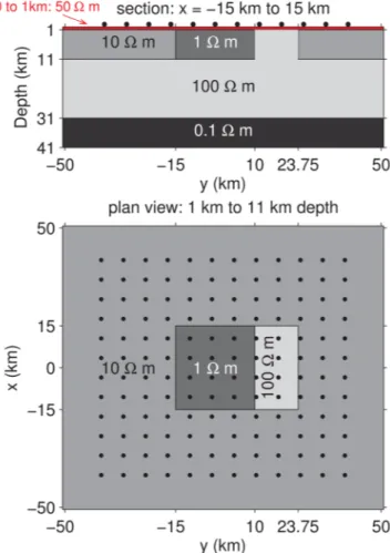
Figure 1.Sketch of the synthetic model used to test the inversion. A section (top) and a plan view (bottom) show the structure of the model. Black dots indicate the locations of MT sites. The site spacing is 7 km.

in March 2011. It was computed for a model which was originally unknown to the participants and was only disclosed at the end of the workshop. Various researchers inverted this data set and a comparison of the inversion results can be found in Miensopust et al.(2013). The model is based on the COMMEMI 3D-2 model (Zhdanovet al.1997), but a 1 km thick, near-surface cover layer of 50m is introduced to avoid numerical problems and effects due to outcropping structure. The lateral dimensions of the two adjacent blocks were also slightly modified. The model is covered with 144 MT sites, located at the surface of the Earth (z=0 km).

The sites are arranged along 12 profiles with equal site spacing of 7 km between sites and profiles. A sketch of the model and the position of the MT sites is shown in Fig.1. The data were simulated for 30 periods in the range from 0.016 to 10 000 s.

Random galvanic distortion has been applied to these data, by multiplying the undistorted impedance tensor by a distortion ma- trixC^obs. The matrixC^obswas calculated according to the Groom- Bailey-Decomposition (Groom & Bailey1989) from randomly gen- erated values for the twist angle (within ±60^◦), the shear angle (within ±45^◦) and anisotropy (within ±1). The gain value was fixed to be equal to one at all locations. Finally, at each site and each individual frequency random Gaussian noise of 5 per cent of the maximum magnitude of the components of the impedance tensor was added to the distorted data. In other words, the noise atjth MT site andnth frequency is equal to 0.05∗r nd∗max

cmp |Zcmp|j n, where cmp=(xx,xy,yx,yy) andrndis a random number drawn from the standard normal distribution.

3-D MT inversion of distorted data 467

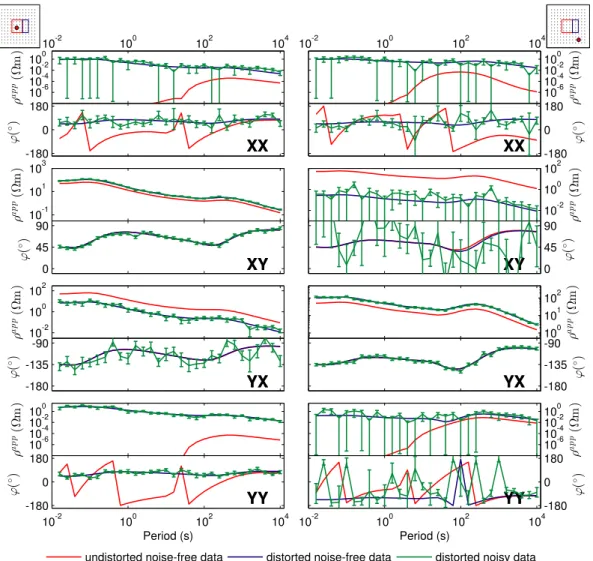
Figure 2. Comparison of undistorted, distorted and noisy distorted apparent resistivities and phases for two exemplary MT sites. From top to bottom each row shows thexx,xy,yxandyycomponents. The left column shows the responses at the site, whose location is indicated by the red dot in the small sketch on the top left. Similarly, the red dot in the sketch on the top right indicates the location of another site, whose responses are shown in the right column. Undistorted data are shown in red, while blue colour represent responses after applying the distortion, green corresponds to the final data, where both distortion and 5 per cent Gaussian noise were applied. Green error bars show the data uncertainties.

The data for two exemplary stations are presented in Fig. 2.

From the figure we see that the distortion not only shifts the off-diagonal apparent resistivities, but also significantly modifies the diagonal elements. Even if the diagonal elements were a few orders of magnitude smaller than the off-diagonal elements before distortion, they can become as large as the off-diagonal elements after distortion. In this case the diagonal elements play as important a role as the off-diagonal ones when inverting the distorted data set.

For more details on the generation of the data see Miensopustet al.

(2013).

For the inversion we divide the volume of interest into 145 × 145 × 14 cells, covering ≈100 × 100 × 70 km³. All cells in horizontal directions have an area of dx×dy= 0.7 × 0.7 km², the vertical cell sizes are growing with depth fromdz1= 250 m to dz14 = 10 km. This model discretization was chosen when the true model was unknown and the cell boundaries do not correspond to the boundaries of the anomalies. Furthermore, the distorted data set was generated with a finite-difference forward modelling solver, while the forward engine for our inversion is based on an integral equation approach. Thus, the numerical errors are different for the observed and predicted data sets.

We use nine periods in the range from 0.063 to 3981 s, since we found that this number of periods is sufficient and the time of the inversion is directly proportional to the number of periods.

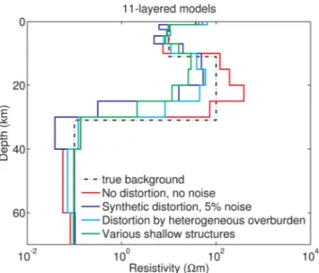
To find the starting model for inversion we compute the averaged Berdichevsky invariant over all sites and than invert it with a 1-D inversion. With this procedure we obtain two 11-layered models, one for undistorted noise-free data and one for distorted and noisy data. These models are shown in Fig.3in red and blue, respectively.

Even though the models do not exactly fit the true background (shown in black), they represent its main features. This technique proved to work well for defining a starting model and in our ex- perience is better than starting the inversion with a homogeneous half-space.

In our first experiment we compare three different inversion runs.

The first run is for undistorted and noise-free data, and we use the standard MT inversion code without distortion correction. For the second and third runs the distorted and noisy data are inverted. For these data we use both versions of the code: (1) the standard MT inversion without distortion correction, and (2) joint inversion of MT impedance data and full distortion matrix. The comparison of the inversion results is shown in Fig.4.

Figure 3.Initial models used for inversion of various data sets. The true background is shown in black. The 11-layered models are generated from a 1-D inversion of the Berdichevsky invariant averaged over all sites. The red line corresponds to the data simulated for model presented in Fig.1, blue line is the same data, but distorted, according to the Groom-Bailey- Decomposition, and with 5 per cent noise added. The cyan and green lines are the starting models for the inversions described in later Sections 3.2 and 3.3, respectively.

For all the inversions presented in the figure, the regularization parameterλwas manually modified during the inversion, starting with a relatively largeλand then gradually decreasing it during the inversion. We run many inversions with various sequences of the regularization parameter and present here only our preferred inversion results. With respect to the trade-off parameterνwe found that the inversion is not particularly sensitive to its value as was also observed by Sasaki & Meju (2006) for their 3-D inversion with static shift correction. For the examples shown in this study, we increased and decreased the value ofνby a factor of 10 and did not observe major changes to the final model or the misfit. For all the runs presented in Fig.4and for our later experiments we therefore use a fixed parameterν=0.01.

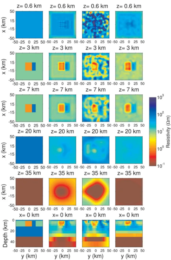
The standard MT inversion code works well on the undistorted data set (second column in Fig.4). Both resistive and conductive blocks are recovered well. The bottom of the conductive anomaly and the bottom of the resistive layer are smeared out and the value of resistivity of the 100m layer is underestimated. However, this is to be expected from a smooth inversion and given the induc- tive nature of MT. In case of inverting highly distorted data, the result of standard MT inversion is not satisfactory (third column in Fig.4). The resulting model has little resemblance to the true model, and contains many small resistive and conductive anoma- lies, especially within the shallow layers of the inversion domain.

More importantly, it is virtually impossible to distinguish the two adjacent blocks. When we apply our joint inversion strategy (fourth column in Fig.4) the two adjacent blocks are clearly seen, and the location and resistivity of the blocks are well resolved. The top layer of 50m and bottom layer of 0.1m are also quite well recovered.

The resistivity of the 100m layer is again slightly underestimated and boundaries of the blocks and layers are smeared out due to reg- ularization. Overall the result is comparable to inverting undistorted data with the standard MT inversion.

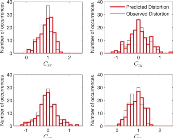
When we include elements of the distortion matrix in the list of the inversion parameters our result is not only a resistivity model but the recovered elements of the distortion matrix as well. The resolved elements of the distortion matrixC^predat each site are presented in Fig.5. To see how well we recover the distortion parameters we also show the elements of the distortion matrix actually applied to the data. The true distortion elements were not known to us before the workshop and were only provided later. From the figure it is seen that the predicted distortion matrix is very close to the true one. The histograms of distortion matrix elements are shown in Fig.6and provide an alternative view on the distortion added to the data and the values recovered by the inversion. Both observed and predicted diagonal elements of the distortion matrix agree well and represent slightly skewed Gaussian distributions around one. The off-diagonal elements of observed and predicted distortion matrix are also in a good agreement and are symmetrically distributed around zero. To analyse the differences in more detail we also calculate relative er- rors between the predicted and observed distortion matrix elements.

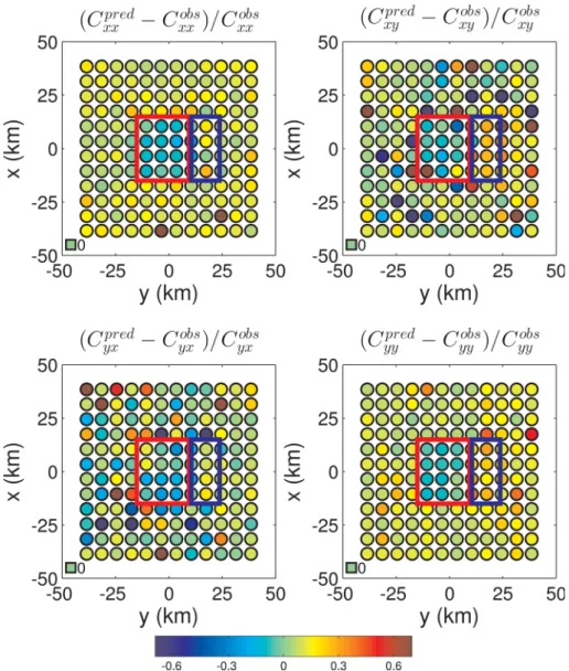
These errors are plotted in Fig.7. The fit is good, especially for the diagonal elements of the distortion matrix. As can be observed from Figs7and5, the largest errors are for the very small elements of the distortion matrix. Even though the fit is good in general, the re- solved elements of the distortion matrix are slightly underestimated below the conductive block and overestimated below the resistive block. This means that a small part of the structural information gets attenuated towards the distortion matrix elements.

The models presented in the second and fourth columns of Fig.4 fit the data to an

RMS= 1

2

N_S

j=1 N_T

n=1

βj ntr

A^T_{j n}Aj n

(11) value of one. However, when inverting the distorted and noisy data with standard MT inversion, the final RMS value does not decrease below≈3.5. To compute the weightsβjnwhich we also use in our objective function (see eq. 3), we assume an error floor ofε=5 per cent of the absolute value of the observed impedance tensorD. In other words,

βj n= 2

NSNTtr

δD^TδD

j n

, (12)

where δD=

max(ε|Dx x|, δDx x) max(εD_{x y}, δDx y) max(εDyx, δDyx) max(εD_yy, δDyy)

. (13)

In eq. (13),δDxx,δDxy,δDyxandδDyyare the error estimates pro- vided with the data.

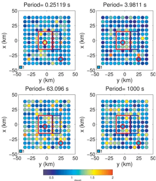
To show how well the joint inversion fits the data at various sites and for four exemplary periods, we plot RMS maps in Fig.8.

These maps also help to understand where we should be careful with interpretation of the inversion results. In general the RMS is around one. Only at the shortest period four sites close to the interface between the two anomalies exhibit significantly larger values of RMS. This is the typical trade-off between smoothness and data misfit in regularized inversion. By tweaking the regularization parameter we could lower the misfit at these sites, but at the expense of over-fitting the data at other sites and periods.

Apart from the higher misfit for the four sites near the inter- face, we do not observe any systematic patterns of over-fitting or under-fitting the data. Both spatially as well as with frequency, the data with RMS above one appear to be randomly distributed as we

3-D MT inversion of distorted data 469

Figure 4. Comparison of the inversion results. The true model is presented in the first column. The second column corresponds to the result of the standard MT inversion of the undistorted and noise-free data. The third and fourth column presents the inversion results for distorted and noisy data set. While the third column is the result of standard MT inversion, the fourth column shows the result of joint inversion, where the elements of the full distortion matrix are sought together with the conductivity distribution. Top five rows show horizontal slices through the model at the depth written above each panel. The last row corresponds to the vertical cross-section through the middle of the inversion results.

Figure 5.The comparison of the elements of the distortion matrixCretrieved by our joint inversion to the distortion actually applied to the data. All the panels show the deviations of the distortion matrix from the identity matrix. Four panels on the left correspond to the distortion matrix as retrieved by our joint inversion, while four panels on the right show the distortion actually applied to the data. The square markers at the bottom left-hand side of the maps are for colour reference.

Figure 6.The comparison of histograms of the elements of the distortion matrixCretrieved by our joint inversion to the distortion actually applied to the data.

3-D MT inversion of distorted data 471

Figure 7.The relative difference between the resolved and the true values of the distortion matrix elements. The colour of the circle corresponds to the value of this difference. The red and blue rectangles show the position of the conductive and the resistive blocks, respectively.

would expect for a least-squares inversion. We also do not observe any obvious correlation of the RMS with the distortion parameters retrieved by the inversion (left-hand panels in Fig.5).

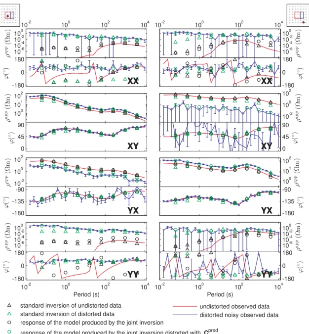
In addition to such RMS maps, it is always useful to look at various components of the data itself. In Fig.9, we present observed and predicted apparent resistivities and phases for two exemplary sites. These sites are also marked by red circles in Fig. 8. From Fig.9we see that the standard MT inversion of the distorted data not only produces a model which is far from the true model, but also fails to fit the distorted data (compare green triangles and blue lines). This is especially evident for the short periods. However, with the joint inversion the fit to the distorted and noisy observed data is good (compare green circles to blue lines). After correcting the predicted data, using the distortion matrix obtained by the joint inversion (black circles) we obtain data which is comparable to the undistorted and noise-free data (red line). For the site presented on the right of the figure and for theyxcomponent, the distortion is slightly overestimated by our joint inversion. On the other hand, for the site presented on the left the predicted distortion is slightly underestimated. However, overall the results of the joint inversion are encouraging.

In practical applications the values and patterns of the data misfit and predicted distortion matrix elements, and the fits to the individ- ual components of the data are the main pieces of information that we can use to assess the quality of our inversion results. The fact that the distortion parameters do not exhibit a regular pattern and are not correlated with the RMS indicates that the inversion is not affected by any systematic bias and the comparison with the true model confirms this.

This first experiment shows that our new joint inversion algorithm is able to recover the resistivity distribution from highly distorted data. However, we also need to check in how far our approach pro- duces significant artefacts when used with undistorted data. Fig.10 presents the result of joint inversion of undistorted and noise-free data. In this experiment, we again use a 1-D layered model pro- duced by 1-D inversion of the averaged Berdichevsky invariant as a starting model for the inversion (see red line in Fig.3). We use a fixed parameter ν = 0.01 and use a cooling approach for the regularization parameterλstarting from 10⁻⁵ and reducing it to 10⁻⁷.

Overall the results from the two algorithms are comparable con- sidering how one would interpret the models if these were field

Figure 8.The data fits for the joint inversion result presented in the fourth column of Fig.4. The colour of the circle corresponds to the value of RMS at this MT site. The period is written above each panel.

data. In particular, the conductive and resistive blocks are resolved well by the standard and joint inversion algorithms. In the deeper parts (>10 km depth) we see remnants of the layered starting model in the joint inversion results (compare to Fig.3). As we explain below, this is a result of the different behaviour of the regulariza- tion in the joint inversion compared to the standard MT inversion.

The distortion matrix obtained by the joint inversion algorithm is close to the identity matrix and therefore we do not present it here.

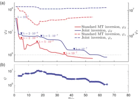
Fig.11presents the comparison of convergence curves of the standard and joint inversions for the case of undistorted and noise- free data. The curves are presented as a function ofnfg. The number nfg is increasing by one after computation of one objective func- tionϕand its gradient _∂{σ,^∂ϕ_C}. We plot convergence with respect to n_fg, rather than with respect to the number of quasi-Newton (QN) iterations, since this number is directly related to the computation time. The number of QN iterations is always smaller thannfg, since the QN optimization at some iterations has to compute the values ofϕand its gradient more than once within the line search. From the figure we see that the standard inversion reaches the target data- misfit of one after 37 objective function and gradient evaluations, compared to 58 for the joint inversion. This is due to the fact that at

the first stages of the joint inversion the algorithm is reducing the data misfit by adjusting the distortion matrix elements and keeping the model nearly unchanged. The functionalψ is growing for the first 17 objective function evaluations, and only then the algorithm is starting to change the model. We think that extra computations are a small price to pay for preventing possible artefacts due to galvanic distortion.

Even though the overall convergence characteristics are similar, the differences in how the data misfit and model regularization terms vary highlight the fact that we are dealing with two different inverse problems. It is therefore not possible to apply identical strategies for choosing the regularization parameterλfor both inversions, since for the same values, the inversions will behave differently. Instead for all examples shown in this study, we run several inversions with different sequences of regularization parameters. From those runs that reach an RMS of one, we choose a preferred model based on its smoothness and fit to various parts of the data. This is similar to the typical strategy one would apply for field MT data.

The differences in convergence behaviour also help to explain the difference between the two inversion results in the deep parts of the models. As the vertical cross-section in Fig.10show, the deep conductive layer is smeared upwards in the standard MT inversion.

3-D MT inversion of distorted data 473

Figure 9. Comparison of predicted and observed apparent resistivities and phases for two exemplary MT sites. The left column shows the responses at the site, whose location is indicated by the red dot in the small sketch on the top left. Similarly, the red dot in the sketch on the top right indicates the location of another site, whose responses are shown in the right column. The responses from three inversion runs are shown: the responses of the models obtained by standard MT inversion of undistorted and distorted data are shown as black and green triangles, respectively, and the responses of the model obtained by the joint inversion of distorted data presented by black circles. The green circles show the responses from the model obtained by the joint inversion distorted with the matrixC^pred. Red and blue curves show the undistorted noise-free and distorted noisy observed data, respectively.

Examining the evolution of models with iteration (not shown here), we see that for the standard inversion the smoothing part of the objective functional reduces the contrasts between the layers of the initial layered model, and makes the deep conductive layer more resistive. Only at the last iterations the conductivity of this layer is increased. The circular structure appears due to the lack of sites above the edges of the presented portion of the model.

The joint inversion works differently. By distorting the data in the initial iterations, the joint inversion improves the data fit and changes the balance between the regularization term and the data misfit term. Therefore, when the inversion starts to work with the model the regularization parameter was already reduced and the balance between the regularization part and the data misfit part is not the same as in case of the standard inversion. The convergence

curves of the regularization partϕsin Fig.11also show that the joint inversion makes much less drastic changes to the model compared to the standard inversion. As a consequence, the layered structure of the starting model can still be seen in the final inversion result.

It is also important to notice that the inversion grid is embed- ded in a layered background with conductivities shown in Fig.3.

For the depths corresponding to the deep conductor, these back- ground conductivities are close to the true conductivity and the circular structure with increased resistivities produced by the stan- dard inversion only occupies a relatively small volume and does not significantly affect the value of the data misfit. In addition, since this circular structure is located outside the array of measurement sites it would not be considered in a practical interpretation of the inversion results.

Figure 10.Comparison of the inversion results. The true model is presented in the first column. The second column corresponds to the result of the standard MT inversion of the undistorted and noise-free data. The third column presents the joint inversion result again for undistorted and noise-free data set. Top five rows show horizontal slices through the model at the depth written above each panel. The last row corresponds to the vertical cross-section through the middle of the inversion results.

3-D MT inversion of distorted data 475

Figure 11. Comparison of the convergences for the standard and joint inversions of noise-free and undistorted data. (a) Convergence of the data misfit,ϕd, and the regularization function,ϕs. The triangular markers show the iterations when we reduce the regularization parameterλ. (b) Convergence of functionψ that keeps galvanic distortion to a minimum.

3.2 Distortion by heterogeneous overburden

In this section, we use the model described in the previous section and shown in Fig.1, but with a heterogeneous overburden. This overburden consists of two 50 m thick layers where the resistivities of each of the 325×325×50 m³cells of these layers are randomly generated from a Gaussian distribution with mean of 1000m and standard deviation of 0.7 in a log scale. In other words resistivity values are 1000×10^0.7∗rnd, whererndis a random number drawn from the standard normal distribution. Fig.12shows a part of the horizontal slice through the first 50 m of the model.

The purpose of this experiment is to use a different mechanism to generate distortion without explicitly generating a distortion matrix C. Instead we try to mimic the structures in the Earth that are thought to be the major source of distortion. However, given the current

Figure 12. A portion of the first layer of the model with heterogeneous overburden. The layers below 100 m are identical to the model shown in Fig.1.

Figure 13. Strength of the galvanic distortion generated by the heteroge- neous overburden of Fig.12. The strength is shown by circles placed in the position of MT sites. Both the size and the colour of the circle correspond to the distortion strength. The black circles show the position of the MT sites shown in Fig.14.

limits in forward modelling, the size of our distorting structures is still larger than what could cause galvanic distortion of real field measurements.

In Fig. 13, we show the strength of the distortion generated by such an overburden plotted as a circle at the position of each MT site. The strength is computed as a Frobenius norm of the difference between the distortion matrix and the identity matrix, tr[(C^obs−I)^T(C^obs−I)]. From Fig.13we see that for most of the sites the difference between the effective distortion matrix and the identity matrix is small, and only about 20 sites have the norm greater than 0.2.

A comparison of the responses of the models with and without the heterogeneous overburden is shown in Fig.14for two exemplary MT sites. The location of these sites is also marked by black circles in Fig. 13. The strength of the distortion of the sites presented on the left and on the right are 0.055 and 0.45, respectively. The left column in Fig.14 demonstrates that even when the norm is small, and therefore the distortion matrix is close to identity, there is a significant effect on the diagonal elements of the impedance at short periods. This is because the undistorted diagonal elements of the impedance at these periods are several orders of magnitude smaller than the off-diagonal elements. Thus, even very small off- diagonal elements of the distortion matrix have a significant effect on the diagonal elements of the impedance tensor, as can also be seen from eq. (1). In contrast, the off-diagonal elements in the left column of Fig.14 are identical for the models with and without

overburden. We observe this behaviour at most of the MT sites. In the right column the distortion strength is relatively large and we observe significant shift of thexy-element of apparent resistivity.

For some MT sites, the distortion generated according to Groom- Bailey decomposition and described in the previous section largely modified the diagonal elements making them as large or even larger than the off-diagonal ones. With the heterogeneous overburden de- scribed in this section, the diagonal elements are also significantly distorted, especially for the short periods, but they still remain less than the off-diagonal elements. We expect that in the case of the field MT data the contribution of the diagonal elements of the distorted impedance tensor can be more pronounced. In its current form the distortion considered in this experiment is a sub-set of the distortion examined in the previous section. It is instructive to see however in how far our inversion approach can deal with such a situation and

Figure 14.Comparison of predicted and observed apparent resistivities and phases for two exemplary MT sites. From top to bottom each row shows thexx, xy,yxandyycomponents. The left column shows the responses at the site, whose location is indicated by the red dot in the small sketch on the top left.

Similarly, the red dot in the sketch on the top right indicates the location of another site, whose responses are shown in the right column. The predicted data are obtained by inversion of the data distorted by heterogeneous overburden. The predicted responses obtained by the standard MT inversion are shown as green triangles, while the predicted data from the joint inversion are circles. Black circles correspond to the responses of the resulting model, and green circles are these responses corrected with the distortion matrix obtained by the joint inversion. The observed data for the model with homogeneous top is shown in red.

And blue colour represent responses for the model with 100 m thick heterogeneous overburden.

3-D MT inversion of distorted data 477

Figure 15. The comparison of histograms of the elements of the distortion matrixCretrieved by our joint inversion to the distortion produced by the heterogeneous overburden.

what the effect on a standard MT inversion is. A similar overburden was considered by Sasaki & Meju (2006) to test their approach to correct for the static shift parameters and thus this experiment also provides some comparability to the results of their study.

We invert the data distorted by the heterogeneous overburden with both standard and the joint inversion. Since the distortion ef- fects caused by the heterogeneous overburden are relatively mild, we do not add noise to the data to be able to see the influence of such a distortion on the inversion. It would be interesting to perform a systematic study with different levels of noise and distortion, but this is out of the scope of this manuscript. As in the previous sec- tion we use nine periods in the range from 0.063 to 3981 s. The starting model for the inversion is again generated by 1-D inversion of averaged Berdichevsky invariant (see cyan line in Fig.3) and the grid dimensions are identical to the previous section. Therefore, the horizontal and vertical dimensions of the inversion grid are not an integer multiple of the forward modelling grid used to generated the synthetic observed data and generally the cell boundaries for the two grids do not coincide. We use a cooling approach for reg- ularization starting withλ=10⁻⁵and reducing it to 10⁻⁷. For the joint inversion we again keep the parameterν fixed and equal to 0.01. Considering an error floor of 2 per cent we fit the observed distorted data to an RMS of one for both the standard and joint in- versions. The resulting data for two MT sites is presented in Fig.14.

Since the diagonal elements of the data are much smaller than the off-diagonal elements for most of the sites and periods we do not fit these data as well as the diagonal ones. For both sites we fit the off-diagonal elements of the distorted data well with both standard and joint inversion. This means that where the effective distortion

is small, for example theyx-component of the site plotted on the right, the standard inversion provides an adequate representation.

However, where we have significant distortion, for example thexy- component of the site plotted on the right, the standard inversion fits biased apparent resistivity values. In contrast, the data corrected by the distortion matrix estimated from the joint inversion lies on top of the undistorted observed data (compare black markers and red line).

In Fig.15we show a summary of the effective distortion matrix elements and the fit by the joint inversion . Overall, the agreement between the histograms of the observed distortion (black) and the distortion recovered by the joint inversion (red) is very good for all four elements. In all cases, we recover the mean and the overall vari- ability of the elements ofC. At some sites, the inversion produces slightly larger values than the observed distortion though. Still, we consider the agreement between observed and recovered distortion values as excellent.

The resulting models are presented in Fig.16. The top layers of the model produced by the standard inversion contain several artefacts (see second column of the figure). These artefacts appear, since the inversion is trying to model the surface inhomogeneities. However, due to the fact that the cell sizes in the inversion are larger than the sizes of the small scale anomalies and due to the regularization, it is impossible to resolve such small features. In contrast to the previous section, the resistivity contrast between these artefacts and the 50m background is not very large and the lower two adjacent blocks are still well seen. The joint inversion helps to clear the top layers of the model from the unnecessary artefacts (see third column).

Figure 16.Comparison of the inversion results for the data produced by the model with heterogeneous overburden. The true model is presented in the first column. The second and third columns correspond to the result of the standard MT inversion and the joint inversion, respectively. Top five rows show horizontal slices through the model at the depth written above each panel. The last row presents the vertical cross-section through the middle of the inversion results.

3-D MT inversion of distorted data 479

Figure 17.Comparison of the inversion results to the true model. The true model is presented in the first column. The second and third column corresponds to the result of the standard MT inversion and the joint inversion, respectively. The panels show horizontal slices through the model at the depth written above each panel.

These tests with distorted data generated through two different mechanisms suggest that our approach can deal with the types of distortion typically encountered in field MT data. As a final test we will investigate in how far correcting for distortion within the inver- sion reduces the ability to image moderate size shallow structures.

3.3 Recovering various shallow structures

In this section, we show the application of the joint inversion to a model containing shallow 10m anomalies of various horizontal sizes. The vertical extent of all structures is 500 m. Other than these shallow structures the model is kept the same as in Section 3.1. The idea is to see which of these anomalies are recovered by the joint inversion and which are substituted by distortion effects. The syn- thetic data were generated using a horizontal cell size ofdx×dy= 1.25×1.25 km²and a vertical mesh withdzgrowing from 500 m to 10 km. For this data set we ran many inversions with various grids and various sets of regularization parameters. Here, we only present the result which in our opinion resolves shallow anomalies the best.

For this inversion, we used a grid consisting of 72×72×14 cells, covering≈100×100×70 km³. All cells in horizontal directions have an area ofdx×dy=1.4×1.4 km², which is coarser than the grid used in the previous sections. The vertical discretization was kept the same as for the other experiments withdzgrowing from 250 m to 10 km. As before, the cell boundaries of the inversion grid and the grid used to calculate the synthetic data do not coin-

cide. The periods were also kept the same and ranging from 0.063 to 3981 s. The initial model for the inversion is again obtained by 1-D inversion and is shown as a green line in Fig.3. In Fig.17we compare the top two layers of the resulting models from standard and joint inversion to the true model. The deeper parts of the model are similar to the inversion results for undistorted data presented earlier.

Both standard inversion and joint inversion retrieve at least some indication of most of the shallow anomalies. The quality of the recovery of these shallow structures is directly related to the site coverage for both inversions. For example, anomaly A is only cov- ered by a single row of sites along the southern edge. In east-west direction the coverage is good and as a result we recover the east- west extent of the anomaly well. However, in north-south direction we only recover the southern half of the anomaly where we have measurement sites. Similar effects can be observed for anomalies C and E. Anomaly D is not recovered by either of the two inversions, as the sites are located right at the boundary of the anomaly.

Another effect that we observe in both inversion results is some interaction of the shallow layers with the two deeper blocks. Over the conductive block on the left the resistivity of the background is overestimated and over the resistive block on the right the resistiv- ity of the background is underestimated. This Gibbs phenomenon is caused by the relatively coarse sampling in terms of MT fre- quencies used in the inversion. Adding more high-frequency data would reduce this effect, but for the purpose of this study it is not particularly relevant.

Figure 18.Comparison of the data fits for the standard and joint inversion results presented in Fig.17. The top row shows the RMS maps obtained by the standard inversion, while the bottom row presents RMS maps for the joint inversion. The RMS values are plotted as circles placed at the position of MT sites and the colours of the circles correspond to the RMS value. The period is written above each panel.

The joint inversion results show essentially the same character- istics as the standard inversion results. The position and extent of recovered anomalies is comparable for anomalies A, B, C and E.

Only anomalies F and G are recovered differently by standard and joint inversions. Anomaly F is not thick enough in case of standard inversion, while the joint inversion correctly recovers the vertical extent of this structure. In contrast, while anomaly G is relatively well recovered by standard inversion, the top of this anomaly is not seen in the joint inversion result. In general, the main difference between two inversion results is that the expression of all anomalies is slightly weaker for the joint inversion. These observations are in agreement with the results of the previous experiments. Including distortion in the inversion tends to produce a resistivity image with less pronounced contrasts at the shallow layers of the model. As a result the smallest shallow anomalies that we can recover with standard inversion are weakened in comparison.

Fig.18compares RMS maps for three exemplary periods for the standard and joint inversions, respectively. Close inspection of the misfit for individual sites and periods reveals that the short periods show an error weighted misfit significantly larger than unity for both inversion approaches. In comparison with the joint inversion though, the standard inversion shows an increased misfit above anomaly D while the joint inversion fits the data satisfactorily. So, in contrast to the joint inversion, the standard inversion provides us with an indication that the model is missing anomaly D. Generally, it is possible to improve the recovery of all anomalies by continuing the inversion with less regularization and improving the data fit.

The price for this is overfitting the long period data and introducing artefacts at depth. It is a general problem in geophysical inversion to balance overall fit with the fit for individual data points and finding suitable strategies is an important challenge for the future.

Thus, when maximum resolution of small near-surface structures is required and the data can be assumed to be free of distortion, the standard MT inversion approach is superior. However, as the pre- vious experiment with small inhomogeneities demonstrates, even a small amount of distortion can affect the recovery of near surface structures. For this reason we consider our distortion correction method a suitable general purpose approach. In most scenarios we expect the safeguard against artefacts from galvanic distortion to outweigh the loss in resolution. In general, it is our experience with geophysical inversion that if some a-priori information is available, for example that the data are not affected by distortion, utilizing this information results in better models.

4 C O N C L U S I O N

Galvanic distortion of MT data is one of the major factors that pre- vents accurate imaging of the subsurface. To circumvent this prob- lem, we have developed and present here a new effective approach that considers galvanic distortion effects during MT inversion. This is achieved by including the frequency-independent elements of the full distortion matrix as additional inversion parameters and adding an extra term to the objective functional which keeps galvanic dis- tortion to a minimum.

3-D MT inversion of distorted data 481 The first two tests consider data with different types of distortion

and demonstrate that we can robustly recover the conductivity of the subsurface and at the same time retrieve information about the galvanic distortion with our new approach. When inverting these data with a standard smooth inversion approach we observe spu- rious artefacts in the inversion results. These artefacts are mostly concentrated in the shallow subsurface, but also hinder the interpre- tation at deeper layers. In contrast, our methodology yields results with a resolution that is close to inverting undistorted data.

To further test our new joint inversion approach we invert undis- torted data. The results of the new approach, in this case, are com- parable to the standard smooth MT inversion. Even though the final models are quite similar, the two algorithms exhibit different con- vergence behaviour, particularly with respect to the regularization term. As a result, the inversion needs more iterations to reach the target RMS and we have to adapt our strategy to choose the regular- ization parameter. In this study we use a simple cooling approach that works for the examples presented here. However, it would be instructive to investigate more generally how the regularization pa- rameter needs to be chosen for a wide range of noise and distortion characteristics. This is out of the scope of this study, but will be the subject of future work.

When trying to image shallow structures of various sizes, we ob- tain similar resistivity models with both standard and joint inversion approaches. Both resulting models only recover small structures that are covered by several measurement sites. In case of the standard MT inversion, although the overall RMS is one, at the sites located close to the missing structures the RMS is significantly greater than one. Therefore, close inspection of the RMS maps at high frequen- cies for the standard inversion points to the missing structures. In comparison, for the joint inversion it is more difficult to identify the missing structures from the RMS maps.

The synthetic tests discussed above suggest that including dis- tortion parameters into the inversion is a promising approach for the general analysis of MT data. However, as all practitioners of MT inversion know though, even the most sophisticated inversion approach can not replace the careful and critical analysis of the observed data and the inversion results. Thus, part of the appraisal of any inversion result has to be an investigation of the impact of the underlying assumptions and parameter choices. It is always valuable to perform many inversion runs with various sets of input parameters and to compare the results with and without distortion correction.

A C K N O W L E D G E M E N T S

We would like to thank the organizers of the 3-D MT Inversion Workshop Pilar Queralt and Alan Jones for simulating the synthetic distorted MT data set and making it available. We also acknowl- edge editors Oliver Ritter and Ute Weckmann and two anonymous reviewers, whose comments and suggestions improved the paper tremendously.

R E F E R E N C E S

Arnason, K., Eysteinsson, H. & Hersir, G.P., 2010. Joint 1D inversion of´ TEM and MT data and 3D inversion of MT data in the Hengill area, SW Iceland,Geothermics,39(1), 13–34.

Avdeev, D. & Avdeeva, A., 2009. 3D magnetotelluric inversion using a limited-memory quasi-Newton optimization,Geophysics, 74(3), F45–

F57.

Avdeeva, A., Avdeev, D. & Jegen, M., 2012. Detecting a salt dome overhang with magnetotellurics: 3D inversion methodology and synthetic model studies,Geophysics,77(4), E251–E263.

Berdichevskiy, M.N. & Dmitriev, V.I., 1976. Distortion of magnetic and electrical fields by near-surface lateral inhomogeneities, Acta Geod.

Geophys. Montanist. Acad. Sci. Hung.,11,447–483.

Bibby, H.M., Caldwell, T.G. & Brown, C., 2005. Determinable and non-determinable parameters of galvanic distortion in magnetotellurics, Geophys. J. Int.,163,915–930.

Caldwell, T.G., Bibby, H.M. & Brown, C., 2004. The magnetotelluric phase tensor,Geophys. J. Int.,158,457–469.

deGroot-Hedlin, C., 1995. Inversion of regional 2-D resistivity structure in the presence of galvanic scatterers,Geophys. J. Int.,122,877–888.

Groom, R.W. & Bahr, K., 1992. Corrections for near surface effects: decom- position of the magnetotelluric impedance tensor and scaling corrections for regional resistivities: a tutorial,Surv. Geophys.,13,341–379.

Groom, R.W. & Bailey, R.C., 1989. Decomposition of magnetotelluric impedance tensors in the presence of local three-dimensional galvanic distortion,J. geophys. Res.,94,1913–1925.

Heise, W., Caldwell, T.G., Bibby, H.M. & Bannister, S.C., 2008. Three- dimensional modelling of magnetotelluric data from the Rotokawa geothermal field, Taupo Volcanic Zone, New Zealand,Geophys. J. Int., 173(2), 740–750.

Jiracek, G.R., 1990. Near-surface and topographic distortions in electro- magnetic induction,Surv. Geophys.,11,163–203.

Jones, A.G., 2011. Three-dimensional galvanic distortion of three- dimensional regional conductivity structures: comment on “Three- dimensional joint inversion for magnetotelluric resistivity and static shift distributions in complex media” by Yutaka Sasaki and Max A. Meju, J. geophys. Res.,116,B12104, doi:10.1029/2011JB008665.

Kelbert, A., Egbert, G.D. & deGroot Hedlin, C., 2012. Crust and upper mantle electrical conductivity beneath the Yellowstone Hotspot Track, Geology,40(5), 447–450.

Miensopust, M.P., 2010. Multidimensional magnetotellurics: a 2D case study and a 3D approach to simultaneously invert for resistiv- ity structure and distortion parameters, PhD thesis, Department of Earth and Ocean Sciences, National University of Ireland, Galway, Ireland.

Miensopust, M.P., Queralt, P. & Jones, A.G. the 3D MT modellers, 2013.

Magnetotelluric 3-D inversion—a review of two successful workshops on forward and inversion code testing and comparison,Geophys. J. Int., 193(3), 1216–1238.

Ogawa, Y. & Uchida, T., 1996. A two-dimensional magnetotelluric inversion assuming Gaussian static shift,Geophys. J. Int.,126,69–76.

Patro, P.K. & Egbert, G.D., 2011. Application of 3D inversion to magnetotel- luric profile data from the Deccan Volcanic Province of Western India, Phys. Earth planet. Inter.,187,33–46.

Patro, P.K., Uyeshima, M. & Siripunvaraporn, W., 2013. Three-dimensional inversion of magnetotelluric phase tensor data,Geophys. J. Int.,192, 58–66.

Sasaki, Y. & Meju, M.A., 2006. Three-dimensional joint inversion for mag- netotelluric resistivity and static shift distributions in complex media, J. geophys. Res.,111,B05101, doi:10.1029/2005JB004009.

Weidelt, P. & Chave, A.D., 2012. The magnetotelluric response function, in The Magnetotelluric Method: Theory and Practice,Cambridge University Press.

Zhdanov, M.S., Varentsov, I.M., Weaver, J.T., Golubev, N.G. & Krylov, V.A., 1997. Methods for modelling electromagnetic fields; Results from COMMEMI—the international project on the comparison of mod- elling methods for electromagnetic induction, J. appl. Geophys., 37, 133–271.