Three–dimensional inversion of transient electromagnetic data: A comparative study

of transient electromagnetic data:

A comparative study

I N A U G U R A L – D I S S E R T A T I O N ZUR

E RLANGUNG DES D OKTORGRADES

DER M ATHEMATISCH –N ATURWISSENSCHAFTLICHEN F AKULT AT ¨

DER U NIVERSIT AT ZU ¨ K ¨ OLN

VORGELEGT VON

M ICHAEL C OMMER

AUS B ONN

K ¨ OLN 2003

Tag der m¨undlichen Pr¨ufung: 12.12.2003

Inversion of transient electromagnetic (TEM) data arising from galvanic types of sources is approached by two different methods. Both methods reconstruct the subsurface three–

dimensional (3D) electrical conductivity properties directly in the time–domain. A principal difference is given by the scale of the inversion problems to be solved. The first approach rep- resents a small–scale 3D inversion and is based upon well–known tools. It uses a stabilized unconstrained least–squares inversion algorithm in combination with an existing 3D forward modeling solver and is customized to invert for 3D earth models with a limited model com- plexity. The limitation to only as many model unknowns as typical for classical least–squares problems involves arbitrary and rather unconventional types of model parameters.

The inversion scheme has mainly been developed for the purpose of refining a priori known 3D underground structures by means of an inversion. Therefore, a priori information is an important requirement to design a model such that its limited degrees of freedom describe the structures of interest. The inversion is successfully applied to data from a long–offset TEM survey at the active volcano Merapi in Central Java (Indonesia). Despite the restriction of a low model complexity, the scheme offers some versatility as it can be adapted easily to various kinds of model structures. The interpretation of the resistivity images obtained by the inversion have substantially advanced the structural knowledge about the volcano.

The second part of this work presents a theoretically more elaborate scheme. It employs imaging techniques originally developed for seismic wavefields. Large–scale 3D problems arising from the inversion for finely parameterized and arbitrarily complicated earth mod- els are addressed by the method. The algorithm uses a conjugate–gradient search for the minimum of an error functional, where the gradient information is obtained via migration or backpropagation of the differences between the data observations and predictions back into the model in reverse time. Treatment for electric field and time derivative of the magnetic field data is given for the specification of the cost functional gradients. The inversion algorithm is successfully applied to a synthetic TEM data set over a conductive anomaly embedded in a half–space. The example involves a total number of more than 376000 model unknowns.

The realization of migration techniques for diffusive EM fields involves the backpropagation of a residual field. The residual field excitation originates from the actual receiver positions and is continued during the simulated time range of the measurements. An explicit finite–

difference time–stepping scheme is developed in advance of the imaging scheme in order to

accomplish both the forward simulation and backpropagation of 3D EM fields. The solution

uses a staggered grid and a modified version of the DuFort–Frankel stabilization method and

is capable of simulating non–causal fields due to galvanic types of sources. Its parallel im-

plementation allows for reasonable computation times, which are inherently high for explicit

time–stepping schemes.

Im Rahmen dieser Arbeit werden zwei Verfahren f¨ur die Inversion von transient–elektro- magnetischen (TEM) Daten von galvanisch gekoppelten Quellen vorgestellt. Beide Meth- oden rekonstruieren die dreidimensionale (3D) Leitf¨ahigkeitsstruktur des Untergrundes im Zeitbereich. Ein wesentlicher Unterschied ist durch die Gr¨oßenordnung des jeweiligen Inver- sionsproblems gegeben. Der erste Ansatz l¨ost kleinskalige Inversionsprobleme und basiert auf bekannten Methoden. Die Rekonstruktion von 3D Modellen mit beschr¨ankter Kom- plexit¨at wird durch die Kombination des Marquardt–Inversionsverfahrens mit einem existier- enden 3D Simulationsalgorithmus f¨ur EM Felder verwirklicht. Das Verfahren ist auf solche Anzahlen von Modellparametern beschr¨ankt, die typisch f¨ur klassische “least–squares” Prob- leme sind. Daher werden eher untypische Arten von Modellparametern eingesetzt, um 3D Strukturen zu beschreiben.

Das Verfahren ist haupts¨achlich daf¨ur geeignet, das Modell einer im Vorfeld grob bekan- nten Untergrundstruktur durch eine Inversion zu verfeinern. Daher sind Vorinformationen eine wesentliche Voraussetzung. Sie werden herangezogen, damit die in ihrer Anzahl be- schr¨ankten Modellparameter so gew¨ahlt werden k¨onnen, dass die interessierenden Strukturen abgedeckt werden. Die Inversionsmethode wird erfolgreich auf Daten einer LOTEM Mes- sung am aktiven Vulkan Merapi (Zentral–Java, Indonesien) angewandt. Trotz der einge- schr¨ankten Modellkomplexit¨at in der Inversion bietet die Methode ein gewisses Maß an Flexibilit¨at. Die Modellparametrisierung kann leicht an verschiedene Untergrundstrukturen angepasst werden. Die Interpretation der Inversionsergebnisse hat wesentlich zum Wissen

¨uber die Verteilung der Leitf¨ahigkeit am Merapi beigetragen.

Der zweite Teil dieser Arbeit stellt ein aus theoretischer Sicht anspruchsvolles Verfahren vor. Es benutzt Techniken, die urspr¨unglich zur Migration seismischer Daten verwendet wurden. Die Methode ist geeignet zur L¨osung großskaliger Inversionsprobleme, die durch komplizierte Modelle mit großer Parameteranzahl entstehen. Der Algorithmus verwendet das Verfahren der konjugierten Gradienten zur Minimierung eines Fehlerfunktionals. Die Gradienten ergeben sich durch Migration der Residuen von gemessenen und durch Model- lannahme berechneten Daten. ¨ Ahnlich wie bei der seismischen Migration bewegen sich die Residuenfelder zeitlich r¨uckw¨arts. Ihre erste Anregung erfolgt zum Zeitpunkt der sp¨atesten Daten und wird bis zum fr¨uhesten Meßpunkt simuliert. Daten von elekrischen Feldern und zeitlicher Ableitung von Magnetfeldern werden in der Herleitung der Gradienten behandelt.

Das Verfahren wird erfolgreich auf einen synthetischen Datensatz angewandt. Dabei wird eine blockf¨ormige Leitf¨ahigkeitsanomalie in einem homogenen Halbraum rekonstruiert. Das Beispiel beinhaltet die L¨osung eines Inversionsproblems mit mehr als 376000 Unbekannten.

Die Anregung der Residuenfelder erfolgt an den Empf¨angerpunkten und setzt sich w¨ahrend

ihrer Simulation fort. F¨ur die Felder der Vorw¨artssimulation und der Migration wird ein

explizites Zeitschrittverfahren speziell f¨ur galvanische Sendertypen entwickelt. Die 3D Sim-

ulation beruht auf einer r¨aumlichen Diskretisierung der Maxwell Gleichungen, die unter dem

Namen ”staggered grid” bekannt ist. Außerdem wird die sogenannte DuFort–Frankel Sta-

bilisierungsmethode benutzt. Explizite Zeitschrittverfahren zeichnen sich durch einen hohen

Rechenzeitbedarf aus. Daher wird der Simulationsalgorithmus f¨ur Parallelrechner entwickelt.

1 Introduction 1

2 Three–dimensional constrained inversion 7

2.1 Methodology . . . . 8

2.1.1 The forward modeling code . . . . 8

2.1.2 The Marquardt–Levenberg inversion scheme . . . . 9

2.2 Synthetic data examples . . . . 13

2.2.1 Inverting for layered background and block resistivity . . . . 14

2.2.2 Inverting for block position and resistivity . . . . 16

2.2.3 Conclusions . . . . 18

2.3 Case history: Mount Merapi, Indonesia . . . . 19

2.3.1 The inverted LOTEM data . . . . 19

2.3.2 A priori information . . . . 21

2.3.3 Constrained mountain model and FD discretization . . . . 23

2.3.4 Stability checks . . . . 26

2.3.5 Results . . . . 29

2.3.6 Interpretation and conclusions . . . . 46

3 A parallel FD scheme for 3D TEM modeling 49

3.1 Methodology . . . . 50

3.1.1 The staggered grid . . . . 52

3.1.2 Time–stepping of the EM field for causal sources . . . . 52

3.1.3 Numerical stability . . . . 55

3.1.4 Boundary conditions . . . . 58

3.1.5 Time–stepping of the EM field for non–causal sources . . . . 60

3.1.6 Parallel implementation . . . . 62

3.2 Synthetic data examples . . . . 66

3.3 Discussion . . . . 74

4 Large–scale TEM inversion 75 4.1 Principles of EM migration . . . . 76

4.2 Background: Maxwell’s equations, Green dyadics and adjoints . . . . 79

4.3 Specification of the gradients . . . . 82

4.3.1 Gradient specification for electric field data . . . . 84

4.3.2 Gradient specifications for voltage and combined data . . . . 88

4.4 Time–stepping backpropagated fields . . . . 89

4.5 Numerical gradient checks . . . . 90

4.6 Solution of the inverse problem by a NLCG scheme . . . . 93

4.7 Solution stabilization . . . . 95

4.7.1 Regularization . . . . 95

4.7.2 Logarithmic model parameters . . . . 96

4.8 Synthetic data inversion example . . . . 96

4.9 Discussion . . . 102

5 Comparative conclusions 103 A Additional notes and derivations 111 A.1 Stability condition for the DuFort–Frankel method . . . 111

A.2 Numerical solution of the 3D Poisson problem . . . 114

A.3 Reciprocity relationship for electric and magnetic fields . . . 116

A.4 Integration order of the gradient . . . 116

A.5 Gradient specification for voltage type data . . . 117

Bibliography 119

Acknowledgments 131

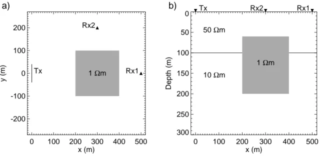
2.1 Model of a 3D conductive body embedded in a two–layered host used to invert for different examples of model parameterizations. (a) Plan view, (b) vertical section. . . . 13 2.2 Synthetic data inversion for the resistivity and position of a block embed-

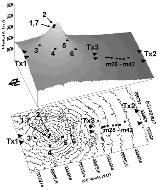
ded in a homogeneous half–space. (a) Plan view and vertical section of the true (shaded rectangle), initial (dashed lines) and final (solid lines) block po- sition of an inversion with conforming block geometry. (b) Synthetic data at Station Rx1 in comparison with initial and final model response for both inverted data sets. (c) Initial and final model results for an inversion with nonconforming block geometry and (d) corresponding data fits. . . . 17 2.3 Digital elevation model and contour map of the survey area. Triangles mark

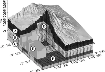
the transmitter electrode points, circles mark receiver positions. . . . 20 2.4 Final 3D resistivity model obtained from MT measurements (after M¨uller, A.,

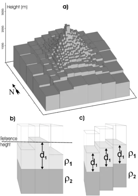
pers. comm.). Here, Merapi is viewed from a SW point. Each letter indicates a region of different resistivity: (A) upper layer, 100 Ωm, (B) intermediate conducting layer, 10 Ω m, (C) conducting layer, 1 Ω m, (D) central conductor, 10 Ωm, (E) SW–anomaly, 1 Ωm, (F) two 2D extended conductors, 0.1 Ωm. . 22 2.5 (a) Modeling of the terrain structure of Mount Merapi with a vertical column

model. (b) Design of horizontal layering. (c) Design of a layering which follows the topography. . . . 24 2.6 Illustration of the approximation scheme used to simulate nonconforming (to

the FD grid) and elongated sources (see Druskin and Knizhnerman [1994]

for further details). (a) Small inclination angles require appropriately small

grid spacings in order to simulate the correct source orientation with respect

to given geographical data included in the FD grid. (b) With an appropriate

transformation of the geographical data, this can be avoided. . . . 25

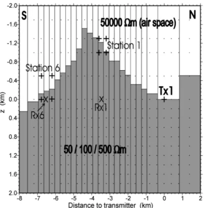
2.7 North–south oriented section of a homogeneous mountain model through the summit. In order to verify FD grid stability, the 3D responses for different mountain resistivities are calculated at Stations 1 and 6 and are compared with the corresponding analytical solutions without topography at the posi- tions Rx1 and Rx6, respectively. . . . 27 2.8 Grid verification results of the 3D volcano model for different resistivity con-

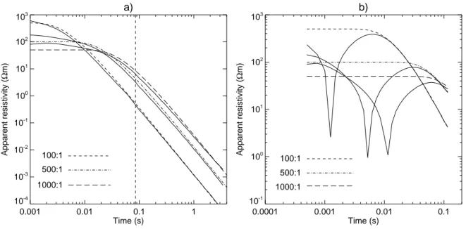
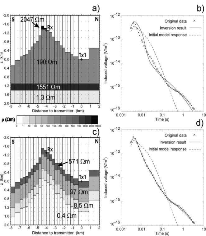
trasts between a homogeneous mountain and the air space (5 10 ⁴ Ωm) for (a) station 1 and (b) station 6. Solid lines are SLDM solutions, dashed lines are analytical solutions over a flat surface. The three curve pairs in each plot correspond to a mountain resistivity of 500 Ωm (contrast 100:1), 100 Ωm (contrast 500:1) and 50 Ω m (contrast 1000:1). . . . 28 2.9 Inversion of a single vertical voltage transient recorded at Station 1. (a) and

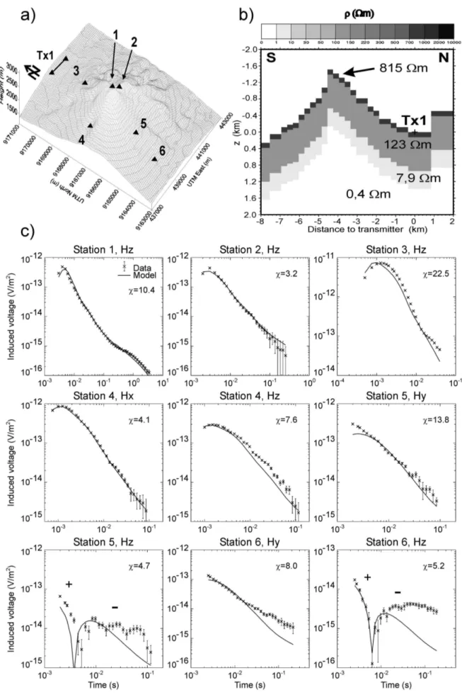
(b) Resulting model and data fit for a horizontally four–layered mountain, respectively. (c) and (d) Resulting model and data fit for four layers which follow the terrain shape. . . . 31 2.10 Joint inversion of the combined data set including Stations 1–6 for a dome–

shaped four–layered mountain model. (a) Transmitter and receiver positions of the combined data set. (b) Resulting mountain model. (c) Final data fits.

The transients are named by the station location and the magnetic component. 33 2.11 Model results from joint inversions of the combined data set (Stations 1–

6) for a dome–shaped four–layered mountain model and an additional block below the summit. The block represents (a) a vertical conduit, (b) a shallow magma reservoir and (c) a deep magma reservoir. Note the larger vertical scale in (c). . . . 35 2.12 Model results from a joint inversion of the combined data set including Sta-

tions 1–7 for a dome–shaped layered mountain model with four layers. (a) Final model result. (b) Final data fit for Station 7. (c) Final data fit for Sta- tions 1–6. . . . 37 2.13 2D pseudo section from 1D inversion results of a southern flank profile [Kal-

scheuer, 2003]. The 1D Occam inversion results are shown for each station with respect to its elevation on the profile. . . . 38 2.14 Model results from a joint inversion of the combined data set including Sta-

tions 1–7 for a dome–shaped layered mountain model with a fault plane be- low the southern flank. (a) Final model result. (b) Final data fit for Station 7.

(c) Final data fit for Stations 1–6. . . . 39 2.15 Transmitter and receiver positions of the stations m28–m42 located on Mer-

api’s southern flank. . . . 41 2.16 Combined inversion of Stations m28–m42. Observed data with both initial

and resulting model response. The upper and lower signs correspond to the

signs of the observed and predicted data, respectively. . . . 43

2.17 Initial and final model producing the corresponding responses in Figure 2.16.

The model parameters are represented by both the lateral and vertical position of the WE–oriented conductive block. The initial and final model are shown in (a) a plan view and (b) a vertical section along the profile. . . . 45

3.1 The 3D staggered grid as used for discretizing Maxwell’s equations. The electric field is sampled at the centers of the prism edges, and the magnetic field is sampled at the centers of the prism faces. (a) Elementary magnetic loops curl around electric fields, (b) elementary electric current loops curl around magnetic fields. (c) Realization of the discrete divergence for mag- netic fields or voltages for a given cell (i,j,k) using the six components of the surrounding cell faces. The corresponding divergence of the current density incorporates the six components of the surrounding cell edges. (a)–(c) also illustrate the communication scheme for the parallel implementation of the field update explained in detail in Section 3.1.6. . . . 53

3.2 Parallel field upward continuation scheme for a distribution of the surface grid layer among four processors. The upward–continuation procedure in- volves remapping, interpolation, forward and inverse 2D FFT steps carried out along both horizontal dimensions x and y of the surface grid layer. The sequence of steps: (a) Initial distribution. (b) Remap, y–interpolation. (c) Re- map, x–interpolation. (d) FFT(x). (e) Remap, FFT(y), upward continuation, FFT ¹ (y), remap, FFT ¹ (x). (f) x–interpolation, (g) Remap, y–interpolation.

(h) Remap to initial distribution. . . . 64

3.3 FD solution (solid lines) over a four–layered host in comparison with an an- alytical solution (dashed lines). (a) Earth model with transmitter–receiver setup. The transmitter is perpendicular to the receiver profile. (b) Electric field response. (c) Vertical voltage response. (d) Horizontal voltage response. 67

3.4 Comparison of the FD vertical voltage (cross symbols) and an analytical (Hanstein, 2003, pers. comm.) solution (solid lines) for a half–space with homogeneous resistivity and a permeable layer (see text for details). Dashed lines show the analytical response over a non–permeable half–space. The transients are calculated for a source–offset of (a) 100 m and (b) 400 m. . . . 68

3.5 FD solution (solid curve) over a homogeneous host with an embedded 3D

block in comparison with an IE solution (cross symbols). The block’s effect

is made visible by the analytical response (dashed curve) over a half–space

without block. (a) Earth model with transmitter–receiver setup. Electric field

responses are calculated at the x coordinates (b) 75 m, (c) 150 m and (d) 225 m. 69

3.6 FD solution (solid lines) from a complex 3D anomaly at a vertical contact and a layered overburden in comparison with a SLDM solution (dashed lines). (a) Earth model. The transmitter is perpendicular to the receiver line. (b) Electric field responses at 100 m, 500 m and 900 m distance from the transmitter. (c) Vertical voltage responses at 200 m, 400 m and 1000 m distance from the transmitter. . . . . 71 3.7 FD simulation of the 3D model from the underground gas storage site at

St. Illiers (France) as derived from a priori information [H¨ordt et al., 2000a].

(a) Section view of the earth model. The transmitter is inline with the receiver profile. (b) Comparison of the electric field FD response (solid lines) with the SLDM solution (dashed lines) at the receiver positions 500 m, 1000 m, 1500 m and 2000 m. (c) Electric field FD response comparisons at 1400 m and 2000 m distance from the transmitter for a downsized reservoir (solid lines) and the full reservoir (dashed lines). To realize the downsized reservoir, the resistivity of the left and right edges (white blocks) is set equal to the resistivity of the surrounding layer. . . . 73 4.1 Illustration of the geometry for the reciprocal relationship between a point at

r in the model space and a receiver at r. Both the external source (Tx) and the receiver (Rx) are electric dipoles. . . . 77 4.2 Checks on the gradients by comparison with a perturbation method. The

contour plots show the absolute differences in % between gradients computed from perturbation and backpropagation. Panel (a) shows comparisons for electric field data, panel (b) shows the corresponding comparisons for vertical voltage data and panel (c) for a combination of both data types. . . . 92 4.3 Transmitter and receiver (R) setup of the synthetic inversion example. Also

shown is the reconstructed conductivity model at the earth surface after 87 iterations. The white rectangle shows the profile of the conductive block buried in a depth of 60 m. . . . 97 4.4 The total normalized (dashed line) error functional is plotted against the in-

version iterations. The solid curve corresponds to the data error component of the normalized error functional. . . . 98 4.5 Reconstructed models in a horizontal plane view at z=100 m (left side) and

data fit for both electric field and vertical voltage data (right side) after 10, 30, 50 and 70 iterations. The shown data corresponds to the receiver position at x=500 m and y=0 m. The true location of the conductive block is indicated by the white rectangle. . . 100 4.6 Reconstructed model after 87 iterations. In each plot the actual location of

the conductive block is indicated by a white rectangle. (a) The x–z cross

section bisects the transmitter at y=0 m. (b) The y–z cross section is located

at x=300 m. (c) The x–y plane of the reconstructed model at 100 m depth. . . 101

A.1 Discretization of the Poisson operator by a seven–point scheme for a grid node (i,j,k) of the 3D mesh. A potential is assigned to each of the seven nodes.

The arrows illustrate the discretization of the right–hand side of the Poisson

equation, involving the current density components of the six surrounding

edges. . . 115

2.1 Inversion results for different data receiver positions and data types. The model parameterization involves the layer unknowns ρ 1 z ₁ and ρ 2 and the block resistivity ρ b . Results 1–6 involve a conforming block geometry, re- sults 7 and 8 a nonconforming geometry. . . . 15 2.2 Inversion results for the data computed at Rx1 from the model shown in Fig-

ure 2.1. In addition to the block parameter ρ b , three layer unknowns are allowed to describe the two–layered background. . . . 15 3.1 Summary of the estimated computation times required by the presented so-

lutions. The factors that govern the computational effort shared between the

n _x

n _y

n _z processors are FD grid size, initial time step and latest simulation

time. . . . 74

I NTRODUCTION

Transient electromagnetic (TEM) methods are made to determine the electrical and properties of the earth. The methods have a well–established place in exploration geophysics, because they have the potential to provide very useful additional information for problems associated for example with mineral exploration [Sarma et al., 1976; Palacky, 1983; Helwig et al., 1994], oil exploration [Spies, 1983; Strack et al., 1989], volcanological hazards [Kauahikaua et al., 1986; Lienert, 1991; Jones and Dumas, 1993] and hydrological investigations [Stewart, 1982;

Mills et al., 1988]. An excellent review of the TEM method and its uses is given by Nabighian and Macnae [1991]. A collection of related publications can be found in the special TEM issue of Geophysics, Vol. 49 (7), 1984.

In the field of environmental geophysics, with shallow exploration depths, TEM methods have become increasingly popular [Frischknecht et al., 1991]. Shallow exploration typically involves systems that employ loops as transmitting antennas with an inductive coupling to the ground. A fundamental description of the physical basis for the TEM sounding technique, with particular attention paid to a configuration where a magnetic receiver coil is located at the center of the transmitter loop (in–loop array), is given by Fitterman and Stewart [1986].

Loop transmitters can be deployed rapidly and more easily than grounded wires. Although the grounded wire is a more complex source, it is often used in deep soundings, because the field falls off less rapidly at large distances and generation of adequate field levels is difficult with loop sources [Spies and Frischknecht, 1991]. The presented work focuses on grounded–

wire transmitters, which have a galvanic coupling to the ground and involve the presence of non–causal source fields. The long–offset TEM (LOTEM) technique [Petry, 1987; Strack, 1992] typically uses a long grounded wire for deep crustal studies [de Beer et al., 1991;

Thern et al., 1996; H¨ordt et al., 2000b] and has been continuously developed at the Institute for Geophysics and Meteorology of the University of Cologne.

In general, data quality and quantity arising from TEM surveys have tended to increase to-

gether with computational capabilities. Therefore, routine interpretation is likely to become multi–dimensional in character. This is important in order to enable multi–disciplinary in- terpretation approaches as a means to achieve earth models with minimum ambiguity in the future. However, the interpretation of TEM data containing effects from multi–dimensional conductivity structures is still non–trivial. First, TEM systems employ artificial sources, which is rather complicated to simulate due to finite source sizes and generation of fields that vary in three dimensions. Second, the solution of multi–dimensional inverse problems is usually large in scale. If arbitrarily complex earth models are taken into account, the number of model unknowns may amount to as much as several tens or hundreds of thousands in real exploration problems.

Therefore, the routine interpretation of TEM data is still based on one–dimensional (1D) earth models (e.g. Macnae and Lamontagne [1987]; Nekut [1987]; Eaton and Hohmann [1989]).

In a 1D inversion (e.g. Anderson [1982]; Raiche et al. [1985]; Huang and Palacky [1991]), a least–squares problem is solved for a conductivity–versus–depth profile of a layered earth model. Different ways of parameterizing a 1D earth exist. For the interpretation of data generated by loop sources Fullagar and Oldenburg [1984] and Farquarson and Oldenburg [1993] use many more layers (with fixed thicknesses) than observations and thus solve an under–determined inverse problem. This greatly increases the non–uniqueness of the mathe- matical solution and thus requires imposing model smoothing constraints in order to generate a model that contains only as much structure as required to fit the data. The inversion for smooth models is also known as the Occam scheme [Constable et al., 1987] and was applied to LOTEM data by Commer [1999]. If, on the other hand, an unconstrained over–determined least–squares problem is solved, one typically allows the variation of both resistivity and thickness of a very limited number of layers, perhaps half–a–dozen. This approach has the potential for generating a plausible representation of the underground, yet the result shows more dependence on the number of free parameters and the starting model. On the other hand, in contrast to smoothing constraints, an unconstrained model is more adequate to incorporate a priori information that may indicate a rich model structure.

In addition to the large–scale difficulties and the complicated 3D source fields, the lack of a sufficient amount of observations may also be a reason for restricting the variation of a model to one dimension. Although the high non–uniqueness problem of a large–scale 3D solution can be addressed by regularization, using smoothing constraints, it still requires an area–wide distribution of detectors above the target to guarantee a reasonable resolution.

However, in many cases, only profiles of observations exist. Such situations suggest to image the lateral variation of the conductivity along the profile direction, in addition to the vertical variation, by means of 2D inversion schemes. At present 2D inversions of direct current (DC) and magnetotelluric (MT) data are common tools and are widely used, whereas the multi–dimensional inversion of TEM data has been developed slower, mainly due to the more difficult simulation of artificial sources. Because of the situation of a 3D source field in a 2D subsurface structure, such inversions for controlled–source methods are often referred to as 2.5D problems [Hohmann, 1988].

Recently, some progress in the solution of the 2.5D EM inverse problem for controlled source

data has been made. Torres-Verdin and Habashy [1994] used the extended Born approxima-

tion for EM tomography. A 2.5D subspace inversion technique based on a finite–element (FE) forward modeling scheme was presented by Unsworth and Oldenburg [1995]. Its effec- tiveness was demonstrated by an application to sea–floor EM surveys. Using a fast integral equation (IE) forward modeling method, Ellis [1998] and Chen et al. [1998] demonstrated the advantage of 2.5D inversions in the interpretation of airborne EM data. Lu et al. [1999]

developed a rapid relaxation inversion of controlled–source audio frequency magnetotelluric (CSAMT) data including the transition–field and near–field data, and Unsworth et al. [2000]

applied this inversion to CSAMT data from a potential radioactive waste disposal site. Mit- suhata et al. [2002] transformed time–domain LOTEM data into the frequency domain and carried out a 2.5D linearized least–squares inversion with a smoothness constraint based upon Bayesian statistics.

The most realistic image of the Earth can be obtained if a model variation in all three Carte- sian dimensions is allowed in an inversion. The development of 2D and 3D inversion schemes for controlled sources has been almost simultaneously, because both types employ 3D source fields. Eaton [1989] formulated an inversion procedure based on frequency–domain, volume integral equations and a pulse–basis representation for the internal electrical field. Using a Born approximation to the 3D IE, Pellerin and Hohmann [1993] iteratively refine a piece–

wise 1D interpretation at a receiver using the data from neighbouring receivers. The EM inverse scattering problem associated with recovering a 3D conductivity model from air- borne TEM data was solved by Ellis [1999], employing a fast IE forward modeling algorithm embedded in a regularized Gauss–Newton optimization driver. Xie and Li [1999] proposed an algorithm for 3D EM inversion that works with the magnetic–field IE, where both forward and inverse IE systems are discretized by the finite–element (FE) method. Zhdanov et al.

[2002] introduced an adaption of the thin sheet method, based on an approximation of the conductivity cross–section by a set of conductive thin sheets with local inclusions.

This work presents two different 3D inversion approaches for time–domain EM data in a comparative study. The first scheme developed in Chapter 2 addresses the large–scale dif- ficulty of full 3D inversion methods. Furthermore, it is optimized for the case when only a limited amount of field data is available for an inversion. The idea of the scheme is to apply an unconstrained least–squares inversion algorithm, usually employed for small–scale uncon- strained 1D problems, to 3D problems. This implies a limitation to only as many model un- knowns as typical for classical least–squares problems. Rather than defining a numerous set of cell–based unknowns given by a simulation grid’s spatial discretization, as is the common approach in large–scale 3D inversions, the shape of larger volumes of constant conductivity is controlled by the model variables. Several different types of untypical model parameters will be shown in the course of Chapter 2. To allow a quick reference, the inversion scheme will also be referred to as SINV ¹ .

The constrained inversion scheme SINV has mainly been developed for the purpose of refin- ing a priori known 3D underground structures by means of an inversion. Therefore, a priori information is an important requirement to design a model such that its limited degrees of freedom describe the structures of interest. Such prior information is often given by geologi-

1 The strong constraints on the model complexity and the limited amount of field data to be inverted suggested

to call the method a “Sparse INVersion”.

cal studies, borehole or other geophysical measurements. An example will be given by a case history from a LOTEM survey at a volcano. Both the mountain topography and lateral con- ductivity variations in the underground require to take 3D structures into account. Because of the mountainous terrain, the survey was made difficult by logistical problems. Therefore, a full large–scale approach is prohibited due to only a sparse distribution of the observa- tions above the target. However, the inversion for “low–parameterized” models involves an over–determined problem and thus makes SINV a practicable tool for the data analysis.

The scheme is based on a stabilized iterative inversion scheme combined with an existing solution for the 3D forward simulation of EM fields. The widely used 3D modeling code developed by Druskin and Knizhnerman [1988] is employed. It has been used a number of times for the 3D simulation of LOTEM responses [H¨ordt, 1992; H¨ordt et al., 2000a;b; H¨ordt and M¨uller, 2000]. The modeling algorithm is based on the spectral Lanczos decomposi- tion method (SLDM) [Druskin and Knizhnerman, 1988; 1994]. The Maxwell equations are solved using Krylov subspace techniques which provides for a fast explicit 3D solver for the diffusion of EM fields in arbitrarily heterogeneous media. The modeling code will be referred to as SLDM code. Its implementation of a material averaging scheme supports the design of arbitrary model parameters. Both the fast 3D forward simulation and the small scale of the inversion problem lead to a relatively low computational effort. The computation time for an inversion is further minimized by distributing the multiple forward simulations during an iteration to several processors of a parallel computer.

In contrast to the constrained inversion scheme, the second part of this work presents a large–

scale inversion approach. The scheme adapts an imaging method originally developed for seismic wavefields [Claerbout, 1971; Loewenthal et al., 1976; Tarantola, 1984] and known as seismic migration to diffusive EM fields. An inversion formulation that applies migration techniques to EM data is not entirely new. Zhdanov and Frenkel [1983] have advanced the idea of migrating or backpropagating the scattered EM field into a homogeneous background medium in order to image the source of the scattering. Lee and Xie [1993] transformed low–

frequency EM fields by an integral transformation into wavefields in order to apply seismic imaging methods. It was along these lines, Wang et al. [1994] developed the theory for solv- ing the full non–linear 3D TEM inverse problem in the time–domain by an efficient way of a conjugate–gradient search for the minimum of an error functional. Zhdanov and Portni- aguine [1997] introduced a new formulation of the time–domain electromagnetic migration technique, based on the minimization of the residual–field energy flow through a profile of observations.

The inversion algorithm presented in this work uses a non–linear conjugate–gradient search

for the minimum of an error functional. While Wang et al. [1994] made much progress

in proposing a tractable approach to 3D TEM imaging, they only applied their solution to

2D synthetic examples from causal sources. This involved the solution of the scalar wave

equation for electric fields and neglected crucial details for implementing the technique for

general 3D imaging. Here, the specifications of the cost functional gradients are formulated

for the full 3D treatment of non–causal source fields arising from galvanic sources. It will

become evident that the problem related to causal source fields is contained in the more

general non–causal case.

The actual solution formulation of the inverse problem by means of migration techniques for diffusive EM fields is outlined in Chapter 4 and involves both forward simulation and backpropagation of the EM field. Therefore, the preceding Chapter 3 develops an adequate explicit finite–difference (FD) time–stepping scheme in order to enable the migration of EM fields, which cannot be realized by the SLDM code. It is in principle based on the FD time–

domain solution for 3D modeling presented by Wang and Hohmann [1993]. However, mainly due to the involvement of 3D non–causal source fields, there are differences in several key aspects as will be outlined in more detail in Chapter 3. Moreover, the solution has been developed for parallel computing platforms.

Preliminary notes

For brevity, following Goldman et al. [1994], in all chapters the word voltage shall be used instead of both “magnetic field time derivative” or “magnetic induction time derivative”. Al- though it may be argued that electric field measurements also effectively involve voltages, it will become clear from the context which kind of field is considered. Vectors and matrices will be represented by bold characters. Lower case characters are used for vectors, upper case letters are used for matrices.

This work treats EM fields generated by sources with a galvanic coupling to the underground.

Such sources and its generated EM fields are also referred to as non–causal. This expression

is chosen due to the presence of a DC electric and magnetic field in the underground before

the source signal is generated by a shut–off. Inductive source types without comparable DC

fields will be referred to as causal.

A 3D CONSTRAINED INVERSION APPROACH AND ITS APPLICATION TO LOTEM ^{DATA FROM}

MOUNTAINOUS TERRAIN

In the geophysical literature, a large number of examples can be found for data interpretation situations, which are characterized as follows:

1. The collected data are insufficient, in terms of the spatial covering of the target, in order to determine a numerous set of model unknowns in a large–scale inversion approach.

This may have several reasons, where logistic and/or economic limitations might be dominant. In other cases, a survey may have the aim of a preliminary investigation of a target and thus involves only a limited amount of measurements.

2. There exists prior knowledge about the target. This can be given by other geophysical disciplines, geological information or borehole measurements. In many cases, TEM surveys are carried out on the basis of a priori information in order to refine the model of an a priori known target (e.g. Taylor et al. [1992]; H¨ordt et al. [2000b]).

3. Simplified 1D inversion approaches fail to take multi–dimensional effects contained in the data into account. Even if a data fit can be achieved, laterally biased interpretations can be expected when 1D methods are applied to the response of more complex struc- tures. Examples where 1D inversions do not accurately recover 2D or 3D resistivtiy distributions are shown by Newman et al. [1987] and Blohm et al. [1991].

Without regard to the complexity of the underground, 1D inversion routines are often em-

ployed, because of the computational expense of a full 3D inversion and the current lack of

available inversion codes for TEM measurements. Even with the capability of inverting for a

large parameter set, the poor resolution due to insufficient data remains. Multi–dimensional forward modeling is often used alternatively (e.g. H¨ordt et al. [1992]; Helwig et al. [1994]).

Starting from an initial guess, a model refinement can be achieved by a trial–and–error proce- dure. However, this method is likely to be more time–consuming, because of erroneous model guesses. Second, such an approach automatically limits the complexity of the earth model, because the manual control of a large set of unknowns is hardly feasible. Finally, a certain amount of experience with the EM responses of multidimensional structures is required.

2.1 Methodology

The inversion method presented in this chapter, also referred to as SINV, is optimized for problems characterized by the above listed aspects. The idea of the scheme is the combination of a Marquardt–Levenberg [Levenberg, 1944; Marquardt, 1963] method as a stable inversion scheme with the 3D forward modeling code from Druskin and Knizhnerman [1988]. The approach addresses the large–scale difficulty by limiting the number of model unkowns to as many unknowns as typical for Marquardt inversions. Inverting for a low–parameterized model involves an over–determined system to be solved. This provides for the capability of resolving multi–dimensional structures even if only a limited amount of field data is available.

The large–scale character of full 3D inversions originates from the usual practice of treating the discrete cells of a finite–difference or finite–element mesh as model unknowns. Such a fine model parameterization quickly leads to a huge set of parameters, but offers a maximum of degrees of freedom during an inversion. Here, the model variation is constrained in a way that a resistivity structure, given by the parameters of the starting model, cannot be changed to a completely new structure. To describe a 3D earth, this involves alternative types of model unknowns, which need to be adapted to the structures of interest. Therefore, it is crucial that sufficient a priori information exists to define proper model parameters. If not present at all, a trial–and–error forward modeling may be the only practical alternative to find a suitable parameterization of the underground. Examples for rather unconventional parameterizations are shown in the course of this chapter. It will be seen that even low–parameterized models can lead to relatively complex 3D structures.

2.1.1 The forward modeling code

The forward modeling code is based on the spectral Lanczos decomposition method (SLDM).

The theory of this solution method is described by Druskin and Knizhnerman [1988; 1994];

Druskin et al. [1999]; a brief summary is also given by H¨ordt et al. [1992]. The solution of the

3D diffusive Maxwell equations by SLDM involves Krylov subspace techniques. Traditional

Krylov subspace techniques include the conjugate–gradient method, biconjugate–gradient

method, and quasiminimal residual methods [Madden and Mackie, 1989; Alumbaugh et al.,

1996; Smith, 1996]. These techniques are very efficient for the solution of large linear systems

with a sparse matrix. The application of SLDM for solving Maxwell’s equations involves

approximating the equations on a spatial FD, thus yielding a system of ordinary differential

equations. The system’s solution is written as the product of functions of its stiffness matrix and the vector describing the initial conditions. The solution on a Krylov subspace can be thought of as a natural extension of the conjugate–gradient method to the computation of arbitrary matrix funtionals [Druskin and Knizhnerman, 1994].

It is crucial that the convergence characterisics of SLDM are taken into account when de- signing a FD discretization for a given earth model. Here, the most important aspects are outlined. A detailed and more theoretical description is given by Druskin and Knizhnerman [1994]. The convergence of SLDM depends on the differential equation system’s condition number, that is the ratio between largest and smallest eigenvalue. The condition number de- pends on the aspect ratio of a FD grid. Ill–conditioning due to a large condition number is introduced by high conductivity contrasts. This results from the requirement that for the ap- plication of SLDM the grid discretization should be fine in conductive regions and coarse in more resistive regions in order to achieve a proper simulation of the attenuation characteristics of EM fields. Hence, convergence problems may occur in the presence of high contrasts if a compromising grid discretization cannot be found. Furthermore, a fine grid should be used to ensure accurate results at early times, whereas low frequency fields need coarse spacings for a quick convergence. Therefore, the simulation of late times also decrease the convergence due to large FD grid aspect ratios.

The forward simulation code allows to define the material properties of the earth, i.e. electric conductivity and magnetic permeability, by means of rectangular blocks. Both conductivity and magnetic permeability do not vary over the block volume. The corners of the blocks are not required to be confined to the cells of the FD grid. However, conductivity contrasts between adjacent blocks should be taken into account when designing the FD grid. The inverse interpolation of the distribution of material properties onto the FD grid is realized by a material averaging scheme described by [Moskow et al., 1999]. This scheme allows to define arbitrary model parameters by the composition of one or more blocks such that they form volumes of constant resistivity.

2.1.2 The Marquardt–Levenberg inversion scheme

The Marquardt–Levenberg inversion scheme (e.g. Jupp and Vozoff [1975]; Lines and Treitel [1984]; H¨ordt [1989]) represents a stable iterative method in the presence of ill–posed inver- sion problems, where small changes in the data can lead to large changes in both the solution and in the process that finds the solution. First consider the classical least–squares approach for inverting a set of observed data for a given earth model parameterization m [Jackson, 1972]. Basically, this involves minimizing the cost functional φ, quantified as the difference between the vectors of the observed and predicted measurements d ^o and d ^p , respectively,

φ m

d ^o

d ^p

^T d ^o

d ^p

(2.1)

which is also called the Gauss–Newton approach [Lines and Treitel, 1984]. The cost func-

tional is connected with a model guess by the implicit dependence of the predicted data on

m. In order to treat the non–linearity of minimization problems related to TEM inversion

problems, the model response

f m

d ^p

is typically assumed to be a linear function of the parameters such that a perturbation of the model response about a given starting model m ₀ can be represented by a first–order Taylor expansion

f m

f m ₀

Jδm

with δm

m

m ₀ defining the model perturbation. The matrix J represents the partial derivatives of the predicted data with respect to the model parameters,

J _{i j}

∂ f i

∂m j

m

m 0

i

1 N; j

1 M (2.2)

and is also referred to as parameter sensitivity matrix or Jacobian. The size of J is N

M, given by the number of observed data points and the number of model unknowns, respec- tively. For the solution of Equation (2.1) it follows [Lines and Treitel, 1984]

δm

J ^T J

¹ J ^T δd (2.3)

where δm now represents the parameter change vector that has to be applied to a model guess m ₀ in order to decrease the data misfit δd

d ^o

d ^p . The linear approximation of the non–linear forward function f involves a step–wise minimum search by evaluating the Gauss–Newton solution (2.3) in an iterative manner, starting from the initial model guess.

The unconstrained least–squares solution (2.3) has the undesirable property of being unstable in the presence of a singular or nearly singular matrix J ^T J. Therefore, the basic strategy of the Marquardt–Levenberg scheme consists of adding a further constraint to the least–squares problem (2.1). To reduce the difficulties with a singular matrix J ^T J, a Lagrange multiplier problem is solved subject to the constraint of a bounded energy of the parameter change, specifically

φ m

δd ^T δd

β δm ^T δm

δm ² ₀

(2.4)

where δm ² ₀ is a finite quantity. The minimization of this functional leads to the so–called damped least–squares solution for the model update [Jupp and Vozoff, 1975]

δm

J ^T J

βI

¹ J ^T δd (2.5)

where the matrix I denotes the identity matrix. The potential singularity of J ^T J is thus re- lieved by adding a constant to its main diagonal ¹ . The degree of damping is controlled by the parameter β . As common practice in Marquardt schemes, for the inversions shown in this work a threshold level is raised by the damping parameter in the first iteration so that only the basic features of the model will be resolved. A gradual decrease of β accounts for less resolved model parameters at later iterations. To define a stopping criteria for an inversion, a lower treshold for the relative error functional decrease, with respect to the previous iteration, is chosen in advance.

1 This can also be understood as adding a DC level to the eigenvalues of J ^T J such that none of the eigenvalues

can vanish.

The presence of data errors assigned to the observations d ^o is addressed by incorporating a weighting matrix W into the minimization problem (2.4). Usually, W is a diagonal matrix, where its entries are the reciprocal values of the standard deviations of d ^o [Jackson, 1972].

Incorporating the data weighting changes the solution in (2.5) to [H¨ordt, 1989]

δm

J ^T W ² J

βI

¹ J ^T W ² δd

(2.6)

The types of model parameters and its small number do not require a further regulariza- tion using smoothing constraints (e.g. Tikhonov and Arsenin [1977]; Constable et al. [1987];

DeGroot-Hedlin and Constable [1990]). However, bounding only the energy of the parame- ter change may still lead to physically unreasonable parameter contrasts. This becomes more severe with the presence of parameters that are poorly resolved by the data. Therefore, the model parameters have to be chosen such that an ill–posedness through irrelevant parameters is avoided. Generally, there is a limit to the number of well defined or important parameters that may be resolved from the data [Jupp and Vozoff, 1975].

Information about the resolution of a model parameter can be obtained from the spectral de- composition of the Jacobian [Jackson, 1972; Jupp and Vozoff, 1975]. H¨ordt [1989] and Petrat [1996] describe the derivation of the so–called importance values from the inversion statistics resulting from the Singular Value Decomposition [Lanczos, 1958] of the Jacobian. Impor- tances represent a means of estimating a model parameter’s degree of resolution and thus help to find the optimal number of parameters. Such importance estimations are employed for the later presented data analysis. Here, it shall only be recapitulated that importances vary between 0 and 1, which means a minimal and maximal resolution of a parameter, respectively.

The calculation of the sensitivity matrix J is usually the most time–consuming part of an inversion procedure, because this requires calculating the variation in the data produced by a change in the model parameters at each iteration. If a perturbation method is employed, each model parameter requires a separate forward simulation for its perturbed quantity. More efficient possibilities exist to calculate parameter sensitivities. McGillivray et al. [1994] cal- culate sensitivities for inversion of frequency–domain data using an adjoint equation method.

A time–domain equivalent for LOTEM data is presented by H¨ordt [1998]. The principles of the adjoint method will be described in detail in Chapter 4. The method is appropriate for a numerous set of unknowns in the form of cell–based grid elements. Here, both the lim- ited number and the types of model parameters suggest the classical perturbation method for calculating the sensitivities.

Data and model parameter transformation

Diffusive EM fields have widely different amplitudes at different times and receiver locations.

To reduce the dynamic range of the data, transformations are preferable in order to equalize

the influence of each datum. Otherwise, the error functional of Equation (2.4) may be domi-

nated by high amplitude data points, thus deteriorating the convergence in an inversion [Meju,

1994]. A simple logarithmic transformation [Jupp and Vozoff, 1975] can be used if all data

points possess the same sign. However, TEM measurements over 3D structures often involve

sign reversals over the measurement time range, thus requiring to distinguish between pos- itive and negative data. Different methods exist to take both large amplitude variations and different signs into account. For example, Wang et al. [1994] use a logarithmic transformation with a linear scale straddling amplitudes near zero and a discrimination between positive and negative logarithms of data values. The transformation scheme realized in SINV is described by Scholl [2001] and is based upon the Area–Sinus–Hyperbolicus function. The funtion has a logarithmic behaviour for arguments 1 or

1 and a linear one for arguments close to zero. This transformation has proven to be suitable for the 1D inversion of LOTEM data containing sign reversals [Scholl, 2001]. Depending on the LOTEM transmitter–receiver ge- ometry and the type of the field component, sign reversals can occur over a 1D earth [Petry, 1987].

An important constraint on model parameters such as electrical conductivity or layer thick- ness is that they must be positive quantities. To enforce this constraint on the inverse solution, a logarithmic transformation is applied to the parameters for all inversions presented in this chapter. A discussion about alternative transformations for parameters describing model fea- tures that can involve negative values will be given at a later stage.

It needs to be taken into account that both data and model parameter transformations carry over to the calculation of the Jacobian in Equation (2.2). Furthermore, the data transformation affects the data errors and thus the weighting matrix W. Scholl [2001] outlines these aspects in great detail for different types of transformations.

Parallel implementation

To update the Jacobian at each iteration makes up the majority of the computational effort for an inversion. It needs one forward simulation for each perturbed model parameter plus one extra simulation for the unperturbed model. The case history in Section 2.3 will show that the forward modeling procedure with the SLDM code may involve more than one FD simulation grid. In this case, the number of forward computations for the model perturbation has to be carried out for each grid.

Calculating the Jacobian can be highly accelerated if a parallel computing platform is used.

As the forward simulations for the perturbed model parameters are carried out independently from each other, they can be distributed among several processors. The optimum number of processors would therefore equal the number of forward simulations required for one itera- tion. This would reduce the computation time by a factor of that number in an ideal case. No inter–processor communication is needed and thus a serial version of the forward modeling code can be used. Communication between the forward simulation code and the inversion algorithm is done via temporary disk files. This way of parallelizing SINV represents not an optimally coded program, because a parallelized version of the SLDM code may be more efficient. However, the implementation is simple achieving a significant gain in computation time. Moreover, as shown by Scholl et al. [2002], this parallelization scheme is also suitable for several stand–alone computers connected by a network.

In a test inversion run, altogether 264 forward simulations were required. A single simulation

needed an average of 2.5 minutes real computation time on a single node of a SUN ^TM Fire 6800 compute server which would sum up to a total time of approximately 11 hours. Using 8 processors this time could be decreased to 2.5 hours.

2.2 Synthetic data examples

In the following SINV is tested on different model parameterizations. Concerning the aspects related to the convergence of SLDM, a stable FD grid for the SLDM code could easily be found, because no excessively high resistivity contrasts are involved in the shown examples.

A more thorough discussion about the preliminary procedure of finding a proper FD grid discretization will be given in Section 2.3. There, designing a stable grid becomes far more difficult due to higher resistivity contrasts. All synthetic data to be inverted for the tests is created by another 3D code presented later in Chapter 3. No artificial noise is added to the data, because here only the case of an optimal data quality shall be treated. The stopping criteria is fulfilled in the case of a relative data misfit decrease dropping below 1 %, relative to the previous iteration. In order to avoid that the inversion finishes too early due to a low relative misfit decrease, a minimum of 4 iterations is enforced.

0 100 200 300 400 500 x (m)

-200 -100 0 100 200

y (m)

Tx Rx1

Rx2

1 Ωm

a)

0 100 200 300 400 500 x (m)

300 250 200 150 100 50 0

Depth (m)

Rx1 Rx2

Tx

1 Ωm 50 Ωm

10 Ωm

b)

Figure 2.1: Model of a 3D conductive body embedded in a two–layered host used to invert for different examples of model parameterizations. (a) Plan view, (b) vertical section.

Consider the 3D model in Figure 2.1. The model represents a 1 Ωm conductive cube embed- ded in a two–layered half–space. The horizontal dimensions of the body are 200 m on a side with a vertical size of 140 m and its depth starting at 60 m. The thickness and resistivity of the upper layer are 100 m and 50 Ωm, respectively, above a 10 Ωm basement. A horizontal grounded–wire source of length 80 m is located at 200 m distance to the block. The example shall demonstrate that SINV is suitable for problems with smaller dimensions of the field–

setup than exemplified in the later shown case history. The data simulated at the receivers

comprises the electric field component in a direction parallel to the source orientation and the time derivative of the vertical magnetic induction _∂ ^∂ _t b z (voltage).

2.2.1 Inverting for layered background and block resistivity

The model parameterization of the first series of inversions assumes the true position and geometry of the block as known in advance and as fixed. Also, the existence of a two–

layered background without its exact structure shall be given as a priori information. The free parameters are thus given by the layer parameters, these are the resistivities ρ 1 and ρ 2 of both layers and the thickness z 1 of the top layer. The fourth parameter is represented by the block’s resistivity ρ b . Altogether 6 inversions are carried out, each one using a different input data set in terms of the receiver position and the data type, where both separate and combined sets are involved.

For each inversion, the input data originates from only a single receiver location in order to simulate the case of a sparse data covering of the target. The inversion results numbered by 1–6 are summarized in Table 2.1. The first and the second line of the table contain the parameters describing the true case and the chosen initial model, respectively. For these examples, all resistivities are initialized to a value of 50 Ωm and the top layer’s thickness is set to a starting value of 50 m. Two different receiver positions are chosen (Figure 2.1), the first one (Rx1) located at a distance of x

500 m from the source without offset along the source axis, the second one (Rx2) at x

300 m and y

200 m. According to Petrat [1996]

and Schneider [2000] these receiver positions do not provide for an optimal resolution of the block anomaly. Thus, the example will also demonstrate that in addition to the sparse amount of inverted data, a reconstruction is still possible with a less optimal receiver configuration.

With the receiver placed at Rx1 and the inversion fed by the electric field data, the true model can be reproduced closely within 12 iterations. The deviation from the true model amounts to only a few percent for each parameter. The voltage data result reveals a worse reproduction of the top layer’s parameters, whereas the basement resistivity is matched. Starting from a value of 50 Ωm, the conductive block is well approximated by a resulting value of ρ b

1 7 Ωm.

The combined data inversion leads to the most exact final model. Apart from a relative difference of approximately 10 % between the true and the reconstructed top layer resistivity, all other parameters show relative errors below 1 %.

In general, inverting the data originating from receiver Rx2 shows larger deviations from the true model. This follows from a worse resolution of the anomalous block, compared to the receiver placed at Rx1. Still a satisfying reproduction of the true underground is achieved by inverting the electric field data during 17 iterations, where also the block resistivity is ap- proximated. However, the voltage data inversion fails to find most of the real model features, with the exception of the basement resistivity. Compared to result 4, the combination of both data types (result 6) produces a similarly good layer model, however with a more erroneous block resistivity.

The electric field data sets of both receivers are sufficient for a reasonable resolution of the

true parameters and are now used in order to exemplify the influence of an erroneous model

Result Rec. pos. Data type Iterations ρ 1 (Ωm) z 1 (m) ρ 2 (Ωm) ρ b (Ωm)

True model 50 100 10 1

Initial model 50 50 50 50

1 Rx1 E x 12 50.8 104.0 9.4 1.1

2 Rx1 B ˙ z 7 63.9 79.1 10.1 1.7

3 Rx1 E _x

B ˙ _z 10 54.5 100.8 9.9 1.0

4 Rx2 E _x 17 49.0 103.1 8.5 2.4

5 Rx2 B ˙ _z 4 243.6 56.1 12.2 39.1

6 Rx2 E _x

B ˙ _z 8 53.2 96.6 9.3 8.7

7 Rx1 E _x 5 175 101.1 32.6 13.8

8 Rx2 E x 10 35.7 55.9 31.1 29.2

Table 2.1: Inversion results for different data receiver positions and data types. The model param- eterization involves the layer unknowns ρ 1 z 1 and ρ 2 and the block resistivity ρ b . Results 1–6 involve a conforming block geometry, results 7 and 8 a nonconforming geometry.

Result Iterations ρ 1 (Ωm) z ₁ (m) ρ 2 (Ωm) z ₂ (m) ρ 3 (Ωm) ρ b (Ωm)

Initial model 50 100 50 100 50 50

1 6 61.8 35.6 39.6 74.3 9.4 1.0

Initial model 100 100 100 100 100 50

2 14 56.7 85.1 59.2 11.9 9.8 1.2

Table 2.2: Inversion results for the data computed at Rx1 from the model shown in Figure 2.1. In addition to the block parameter ρ b , three layer unknowns are allowed to describe the two–layered background.

parameterization. Using the input data produced by the original model shown in Figure 2.1, the model guess is now characterized by a nonconforming block geometry. Instead of a volume of 200

200

140 m ³ , the block is assumed to have a fixed volume of 300

300

200 m ³ , where its center position is kept. Due to the larger volume, erroneous results are obtained for each inversion as shown in the results 7 and 8 in Table 2.1. However, except for the top layer’s final resistivity of each result, all parameters show a trend towards the correct solution, with respect to the starting model. Even the true thickness of the overburden is found by inverting the data of Rx1. Compared to the real values, the larger block volume causes increased values for the resulting block resistivity.

Another test for a less conforming model parameterization involves the assumption of a

three–layered background, thus inverting for 5 layer parameters. An additional unknown

is again represented by the cube’s resistivity with the true geometry given. The joint data set

of Station Rx1 generated by the two–layered model in Figure 2.1 is used for this test. All

initial resistivities are set to a value of 50 Ωm. Both layer thicknesses start with values of

100 m. First, it can be seen from Table 2.2 (result 1), that the block resistivity is matched

exactly. However, both final layer resistivities ρ 1 and ρ 2 differ by approximately 10 Ωm from

the true case, despite correct initial values. Nevertheless, the two–layered background can be

recognized. The sum of both thicknesses z 1 and z 2 shows the original vertical location of the

basement’s beginning with a deviation of 10 %. Its true resistivity of ρ 3

10 Ωm is closely matched.

A similar inversion (result 2) uses the initial resistivities of 100 Ωm for ρ 1 , ρ 2 and ρ 3 . In general, the final model result is better than given by the previous inversion. However, both resistivity values ρ 1 and ρ 2 still show differences of 13 % and 18 %, respectively, from the true value of 50 Ωm. The overburden thickness is reconstructed by the sum of z 1 and z ₂ with an error of only 3 %. The resistivity ρ 3 of the layer below the overburden and the block’s resistivity ρ b are reproduced to a satisfying degree as well.

2.2.2 Inverting for block position and resistivity

The following two inversions involve a model parameterization that is different from the more common types of parameters given by layers or blocks. The combined data of electric field and voltage at Station Rx1 is inverted. It is generated from a 50 Ωm homogeneous half–space with an embedded anomalous block as the one shown in Figure 2.1. No layer parameters are defined for these inversions, thus a fixed 50 Ωm background shall be assumed in the inversion. In addition to the block’s resistivity ρ b , the model parameters are now represented by its center coordinates x y and z along each cartesian axis, thus four unknowns exist. The starting model for the first inversion example assumes a 50 Ωm block with its true size also known.

As shown by the plan view and vertical section of Figure 2.2a, the initial model (dashed rectangles) is characterized by a 100 m offset from the true position for both horizontal coor- dinates x and y and a 40 m offset from the true depth. The solid lines mark the resulting block location after 8 iterations. The inversion moves the initial block towards the original location (shaded rectangle) such that a good agreement along both the x axis and the vertical axis is achieved. The only significant deviation of approximately 20 m from the true position occurs along the y axis. The block’s resistivity of 1 Ωm is reproduced exactly in this example. For both data components Figure 2.2b shows the synthetic data generated by the original model in comparison with both the initial response and the response calculated from the solution.

Apart from slight deviations at the latest times of the electric field data, both predicted data curves show a good agreement with the original data.

In order to exemplify another inversion with a less conforming parameterization, the block’s geometry is now assumed to be 50 m larger along each dimension, as illustrated by the dashed rectangle in Figure 2.2c. Also, the starting position is shifted farther away from the true po- sition, such that its center coordinates differ by values of ∆x

225 m, ∆y

225 m and

∆z

265 m from the true center point coordinates. The final model result reveals a suc-

cessful inversion, because the real block is enclosed by the borders of the larger block after

9 iterations. Similar to the previous example involving a nonconforming block geometry (re-

sults 7 and 8 in Table 2.1), the larger block volume causes a trend towards the resistivity of

the background. The initial block resistivity of 50 Ωm is decreased to a value of 7.2 Ωm. To

Figure 2.2: Synthetic data inversion for the resistivity and position of a block embedded in a homo-

geneous half–space. (a) Plan view and vertical section of the true (shaded rectangle), initial (dashed

lines) and final (solid lines) block position of an inversion with conforming block geometry. (b) Syn-

thetic data at Station Rx1 in comparison with initial and final model response for both inverted data

sets. (c) Initial and final model results for an inversion with nonconforming block geometry and (d)

corresponding data fits.