1. Introduction
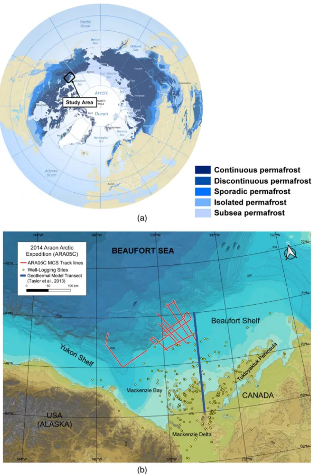
Since the Last Glacial Maximum (∼19 ka), the sea level has risen at least 120 m, flooding the coastal perma- frost regions of the Arctic Ocean (Hill et al., 1985). The submerged permafrost has since then been exposed to warmer temperatures and has been slowly melting. Figure 1a shows the map of the circum-Arctic perma- frost distribution (Brown et al., 1997). Recently, the consequences of rapid climate change and warming in the Arctic have become a significant topic of public concern and scientific debate (Chadburn et al., 2017).
Detailed information on the distribution of permafrost beneath the seafloor of the continental shelves throughout the Arctic is essential for detecting and quantifying potential sources of methane release, which can further accelerate global warming (Archer et al., 2009; Ruppel, 2011; Shakhova et al., 2010).
Since subsea permafrost was initially discovered in industrial boreholes in the Beaufort Sea (Mackay, 1972), several research programs for the investigation of subsea permafrost have been conducted based on the geophysical characteristics of frozen or icy media. In the Canadian Beaufort Sea (CBS), geophysicists have identified the widespread occurrence of subsea permafrost using seismic refraction methods (Hunter et al., 1974). Pullan et al. (1987) analyzed seismic refraction data and developed a map showing the distri- bution of subsea permafrost on the continental shelf of the CBS. A classification scheme for ice-content the sediments based on characteristic ranges in seismic refraction velocities was developed with velocity values
Abstract
Climate change in the Arctic has recently become a major scientific issue, and detailed information on the degradation of subsea permafrost on continental shelves in the Arctic is critical for understanding the major cause and effects of global warming, especially the release of greenhouse gases. The subsea permafrost at shallow depths beneath the Arctic continental shelves has significantly higher P-wave velocities than the surrounding sediments. The distribution of subsea permafrost on Arctic continental shelves has been studied since the 1970s using seismic refraction methods. With seismic refraction data, the seismic velocity and the depth of the upper boundary of subsea permafrost can be determined. However, it is difficult to identify the lower boundary and the internal shape of permafrost. Here, we present two-dimensional P-wave velocity models of the continental shelf in the Beaufort Sea by applying the Laplace-domain full-waveform inversion method to acquired multichannel seismic reflection data. With the inverted P-wave velocity model, we identify anomalous high seismic velocities that originated from the subsea permafrost. Information on the two-dimensional distribution of subsea permafrost on the Arctic continental shelf area, including the upper and lower bounds of subsea permafrost, are presented. Also, the two-dimensional P-wave velocity model allows us to estimate the thawing pattern and the shape of subsea permafrost structures. Our proposed P-wave velocity models were verified by comparison with the previous distribution map of subsea permafrost from seismic refraction analyses, geothermal modeling, and well-log data.© 2021 Her Majesty the Queen in Right of Canada. Reproduced with the permission of the Minister of Natural Resources.
This is an open access article under the terms of the Creative Commons Attribution-NonCommercial License, which permits use, distribution and reproduction in any medium, provided the original work is properly cited and is not used for commercial purposes.
Inversion
Seung-Goo Kang1 , Young Keun Jin1 , Ugeun Jang2 , Mathieu J. Duchesne3 , Changsoo Shin4, Sookwan Kim1 , Michael Riedel5 , Scott R. Dallimore6,
Charles K. Paull7, Yeonjin Choi1,8, and Jong Kuk Hong1
1Division of Earth Sciences, Korea Polar Research Institute, Incheon, Korea, 2Department of Geological Sciences, Chungnam National University, Daejeon, Korea, 3Geological Survey of Canada, Quebec, QC, Canada, 4Department of Energy Resources Engineering, Seoul National University, Seoul, Korea, 5GEOMAR Helmholtz Centre for Ocean Research, Kiel, Germany, 6Geological Survey of Canada, Sidney, BC, Canada, 7Monterey Bay Aquarium Research Institute, Moss Landing, CA, USA, 8Department of Energy Resources Engineering, Korea Maritime and Ocean University, Busan, Korea
Key Points:
• The P-wave velocity models have been successfully calculated for imaging the subsea permafrost by applying the full waveform inversion
• The inverted models were verified and interpreted with the results of previous related studies for the subsea permafrost
• The detailed shapes, sizes, and lower boundaries of the subsea permafrost can be estimated by inverted models
Correspondence to:
J. K. Hong, jkhong@kopri.re.kr
Citation:
Kang, S.-G., Jin, Y. K., Jang, U., Duchesne, M. J., Shin, C., Kim, S., et al. (2021). Imaging the P-wave velocity structure of Arctic subsea permafrost using Laplace-domain full-waveform inversion. Journal of Geophysical Research: Earth Surface, 126, e2020JF005941. https://doi.
org/10.1029/2020JF005941 Received 19 OCT 2020 Accepted 8 FEB 2021
Special Section:
The Arctic: An AGU Joint Special Collection
Figure 1. The map of the study area: (a) is a Circum-Arctic map of permafrost distribution (modified from Brown et al., 1997), and (b) is the map of our study area in the southern CBS in the 2014 ARAON Arctic expedition.
lower than 2.5 km/s representing ice-free sediment (Pullan et al., 1987). Recently, the minimum extent of subsea permafrost distribution on the U.S. continental shelf of the Beaufort Sea has also been estimated using seismic refraction analyses (Brothers et al., 2012). Following Johansen et al. (2003), the theoretical seismic velocities of subsea permafrost range are less than 2.8 km/s for saturated sands with less than 40%
ice content (i.e., the proportion of ice filling the pore space) and from 3.4 km/s to as high as 4.35 km/s for sediments with 40%–100% ice content.
Subsea permafrost has, in general, higher P-wave velocity than the surrounding sediments at shallow depths, and refraction events generated by the upper boundary of subsea permafrost have been confirmed even in seismic data with very short offsets. Seismic P-wave velocities can be determined through the anal- yses of refracted seismic arrivals in shot-gathers, allowing permafrost to be readily detected, and the depth to the upper boundary of permafrost can be estimated from the crossover distance (i.e., where the refracted and direct arrivals intersect) under the assumption of horizontal interfaces (Hunter et al., 1976; Rogers &
Morack, 1980). However, detecting the lower boundary and thus the thickness of subsea permafrost is very difficult because it is impossible to generate a refracted event from an interface between two layers when the lower layer has a lower velocity (Hinz et al., 1998). Also, shallow water depth on the Arctic continental shelf and the abnormal high velocity of subsea permafrost structures located just below the seafloor generate complex multiples in the seismic records. Water-column seafloor multiples are difficult to eliminate using conventional signal processing or de-multiple techniques in this case, because of the shallow water depth under 50 m of the inner shelf area. Internal multiples from the subsea permafrost structures with high velocity, located in subseafloor combined with the shallow water depth of the continental shelf, are also a severe obstacle for imaging subsurface geological structures from the seismic data. These multiples make the process of picking velocities reliably within a seismic semblance panel ambiguous. Therefore, the con- ventional seismic velocity analysis has limitations for building an accurate P-wave velocity model of subsea permafrost structures. However, the seismic P-wave velocity is the fundamental property for distinguishing the subsea permafrost from the normal sediments because the P-wave velocity increases noticeably when the ice content exceeds 40% (Johansen et al., 2003). Thus, we note that finding a method for getting accurate two-dimensional P-wave velocity models from the seismic data is the crucial point for advanced research of subsea permafrost on the Arctic continental shelf.
In this study, we propose two-dimensional P-wave velocity models for imaging subsea permafrost structures obtained by using the acoustic full-waveform inversion method applied to multichannel seismic (MCS) data acquired over the continental shelf of the CBS (Figure 1b). Here, we use the Laplace-domain full-waveform inversion (LFWI) method introduced by Shin and Cha (2008) to construct an accurate P-wave velocity model of subsea permafrost structures. The LFWI is known for being one of the most reliable methods for building P-wave velocity models from field data and has been previously used for identifying high-velocity structures, such as salt domes, that represent a rapid increase in seismic velocities similar to the subsea permafrost environments (Ha et al., 2010; Shin & Cha 2008, 2009). Kwon et al. (2017) suggested a way for constructing an accurate P-wave velocity model from the seismic data by the LFWI using the Hessian matrix of the Gauss-Newton method. The Hessian matrix in the LFWI algorithm specialized in the correction of the depth for high-velocity structures in the inverted model as following the Kwon et al. (2017)'s approach.
We adopted the Gauss-Newton method to consider the Hessian matrix for the LFWI to build a represent- ative P-wave velocity model of the subsea permafrost. The raw seismic data are preprocessed by applying noise attenuation procedures and the Laplace-transform prior to applying the LFWI. Inverted P-wave ve- locity models are constrained by a comparative analysis with previous studies, including seismic refraction analysis, geothermal modeling, and well-logging data. Finally, the two-dimensional distribution and the geophysical characteristics of the subsea permafrost are derived by the interpretation of the inverted P-wave velocity models.
2. Review of the Laplace-Domain Full-Waveform Inversion Method
The LFWI scheme allows the reconstruction of seismic velocity models from seismic field data. The LFWI, which is based on the two-dimensional acoustic wave equation, is an established technique for reconstruct- ing P-wave velocity models from the Laplace-transformed wavefields of seismic data (Shin & Cha, 2008).
Below, we briefly review the LFWI method for acoustic media with simple equations to explain the basic concepts of the algorithm.
The Laplace-transformed acoustic wave equation can be defined as:
2 2 2
2 2 2
s p p p f
c x z
(1)
where s is the damping coefficient of the Laplace transform; p(x, z, s) is the Laplace-transformed pressure field in two-dimensional acoustic media; c is the P-wave velocity in the acoustic media; and f is the source term. The discretized finite-element formula of the wave equation in the Laplace domain was represented by the impedance matrix formulation as follows:
, Su f
(2)
2 .
S Ms K
(3) where impedance matrix of the discretized wave equation for acoustic media S consists of the mass matrix M and the stiffness matrix K, as shown in Equation 3; u is the Laplace-domain wavefield vector of the pres- sure field p; and f is the Laplace-transformed source vector (Marfurt, 1984; Shin & Cha, 2008).
The first step of the inversion procedure is defining the objective function. In the LFWI, the logarithmic objective function, proposed by Shin and Min (2006), is used for measuring the residual between the mod- eled data and field data. The logarithmic objective function is more useful than the conventional l2 objective function for measuring the residuals (Shin & Cha, 2008; Shin & Ha, 2008) in the LFWI algorithm because the Laplace-domain wavefield has very small absolute values. The logarithmic objective function G for our LFWI algorithm can be described as follows:
1 1
1 2
n ns r ij ij
G i j r r
(4)
ij ln ij
ij
r u
(5)d
where dij, uij and rij are the observed wavefield, the modeled wavefield, and the residual at the jth receiver by the ith source, respectively. ns and nr are the total numbers of sources and receivers of the acquired seis- mic field data. In order to calculate the gradient direction of the objective function, the back-propagation algorithm (Tarantola, 1984) is used.
In Equation 6, gradient direction with respect to a model parameter k(ix,iz) is described by the back-propaga- tion algorithm as follows:
,
, 1 G , Re ns1 T
kix iz ix iz i fvkix iz S ri
(6)
where, ix and iz are indices of the x-axis (horizontal direction) and z-axis (depth or vertical direction) ele- ments of the modeling media, fvk ix iz , is the virtual source term defined as
, ,
kix iz i,
ix iz
fv S u
(7)k
where ui is the forward modeled wavefield and r can be defined asi
r
u d u
u d u
u d u
i
i i i
i i i
i nr i nr i nr
ln / /
ln / /
ln , / , / ,
1 1 1
2 2 2
0
0 0
(8).
After calculating the gradient direction of the LFWI objective function, the model parameters (Pyun et al., 2011) are updated as:
1, , ,
,
, 1
1
Δ
G , .
H , I
l l
ix iz ix iz ix iz
nf k ix iz
lix iz s ns
i
k k k
ix iz k
ix iz
(9)
where l is the iteration number, Δk ix iz, is the perturbation to the model parameter, nf is the total number of Laplace damping constants, H is the Hessian matrix (Pyun et al., 2011), and I is a stabilizing factor. The unknown source wavelet was calculated by the source estimation algorithm based on the Newton method (Koo et al., 2011).
In previous research, the LFWI algorithm was verified for constructing meaningful velocity models from seismic field data sets by comparing it with other waveform inversion algorithms (Bae et al., 2012; Ha &
Shin 2012; Kang et al., 2012; Shin et al., 2010). Especially, the LFWI algorithm is known for working well with inversion targets such as salt domes with significantly higher velocities than the surrounding sediment or rapidly changing velocity areas. Recently, Kwon et al. (2017) found that the LFWI results sometimes suf- fer from a gradient distortion effect known as a shifted-down targeted structure in the results of the LFWI scheme. It means that the inverted P-wave velocity structures were constructed at a deeper depth than the actual depth. Notably, this effect is known to occur in LFWI procedures for high-velocity structures, such as salt domes. They suggested a solution for the gradient distortion encountered in LFWI using the Hessian matrix of the Gauss-Newton method calculated by the conjugate gradient least squares (CGLS) approach.
The correlation terms between the partial derivative wavefields were composed of the Hessian matrix. In the Gauss-Newton method, the Hessian matrix plays a role in the scale factor for velocity update procedure in the LFWI algorithm as shown in Equation 9 and make it possible to perform the stable waveform inver- sion in the Laplace domain even though extremely high-contrast velocity structures were located in the in- version targets (Kwon et al., 2017; Pyun et al., 2011). In this study, we applied two-dimensional LFWI by the Gauss-Newton method and employed it to calculate accurate P-wave velocity models for subsea permafrost from field-acquired seismic data without the gradient distortion effect. A flowchart of the LFWI technique is presented in Figure 2 to provide detailed information for the process of the LFWI algorithm.
3. Numerical Test of the LFWI on a Synthetic Data Set for the Imaging the Arctic Subsea Permafrost
In previous LFWI studies, seismic data recorded using a long streamer of 8 km or longer were used to test the applicability of the algorithm to field data for verification of the LFWI algorithm. The targeted subsur- face structures located in 3–5 km depth were reliably reconstructed in the inverted velocity models (Ha
& Shin 2012; Ha et al., 2010; Kwon et al., 2017; Shin & Cha 2008, 2009). In this study, seismic data were recorded in the CBS in 2014 with a relatively short (total length of 1.5 km) streamer with 120 channels. The main imaging targets of this study are permafrost structures, presumably exhibiting considerably higher P-wave velocities than the surrounding sedimentary layers. The water depth is approximately 50 m for the
study area, and the permafrost structures are generally known to be located from 50 m beneath the seafloor to a maximum of 600 m depth in the shelf area as following previous research (Taylor et al., 2013) in the CBS area. Therefore, we need to confirm the possible imaging depth of the LFWI algorithm for the acquired seismic data. Also, it is necessary to verify whether the LFWI technique can reconstruct a representative P-wave velocity model in shallow water depths (less than 50 m) with abnormal high-velocity structures located just below the seafloor.
We tested the applicability of LFWI using a synthetic data set generated from the velocity model shown in Figure 3a by time-domain wave propagation modeling. The test model was designed based on information provided by a previous study on the subsea permafrost distribution (Taylor et al., 2013). The dimensions of the test model were 100 km long with the 1 km in-depth, including a 50 m-deep water layer. The inversion target is a high-velocity structure (P-wave velocity of 3.0 km/s) that was located at depths ranging from 100 to 600 m in the true-velocity model. The synthetic data set contains the modeled seismic signal from a 120-channel streamer with a 10-m group interval. The shot interval was 50 m, the total recording time was 7 s, and the sampling rate was 1 ms, which is similar or the same as the field data acquisition in the 2014 expedition on CBS. For the waveform inversion, the model grid size of the inverted model was 10 m. The constrained minimum and maximum inverted velocities were set to 1.45 and 3.0 km/s, respectively.
For the initial velocity model, the P-wave velocity of the water layer was fixed to 1.45 km/s for a water depth of 50 m, the same as in the true-velocity model. We set a constant initial velocity (2.4 km/s) for the initial model to begin LFWI in this synthetic numerical test, as shown in Figure 3b. The calculated gradient direc- tion of the objective function at the first iteration for LFWI is shown in Figure 3c. In the model of gradient direction, a positive gradient means that the P-wave velocity value is lower in the next iteration, and a nega- tive gradient implies that the P-wave velocity value is higher in the next step. The gradient direction signifies the trend of the velocity update from the initial model to the next iteration. We can estimate the location, Figure 2. Flowchart of the Laplace-domain full-waveform inversion (modified from Shin & Cha, 2009).
shape, and actual size of the target structures in this gradient direction model at the early stage of the LFWI procedure. Figure 3d shows the inverted P-wave velocity model from the synthetic data set by LFWI. In the inverted model, we note that the target structure was successfully reconstructed in the inverted model located at depths from 100 to 600 m. Additionally, the low-velocity area in the upper part of the true-model is well-reconstructed in the inverted model, as shown in Figure 3d. Notably, the shape of the high-velocity structure was well reconstructed, and the lower boundary of the high-velocity structure can be defined as 600 m, even though the streamer length of 1.5 km was relatively short and the water depth was shallow (less than 50 m). From this synthetic test of LFWI, we confirm that LFWI can be applicable to seismic data acquired in 2014 on CBS to image subsea permafrost structures.
4. Imaging the P-Wave Velocity Structures of Subsea Permafrost on the CBS
4.1. Seismic Data
Seismic data were collected onboard the icebreaking research vessel (IBRV) ARAON in 2014 to investigate the geophysical characteristics and distribution of subsea permafrost beneath the seafloor of the CBS off the coastline of the Northwest Territories. The map in Figure 1b is the map showing the entire study area of the 2014 expedition, including MCS tracks, the location of industrial wells, and the transect line of the geothermal model proposed by Taylor et al. (2013). The map in Figure 4 shows the two seismic tracks (“ARA05C-05” and “ARA05C-17,” marked with solid-red lines) for applying to the LFWI algorithm and the classification of four areas for the distribution of subsea permafrost in CBS proposed by Pullan et al. (1987).
The acquisition system of the MCS data used in the 2014 survey included a 120-channel streamer with an active length of 1.5 km and an airgun array with a total volume of 19.7 L. The shot and group intervals were 50 and 12.5 m, respectively. The schematic diagram and detailed data acquisition parameters for the 2014 seismic survey on CBS are shown in Figure 5.
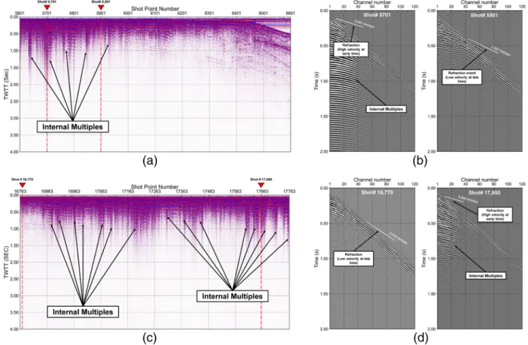
The common-offset and shot-gathers for survey lines “ARA05C-05” and “ARA05C-17” are shown in Fig- ure 6. Figures 6a and 6c are the common-offset gathers of the first channel containing the internal multi- ples with high amplitudes just below the seafloor. These internal multiples, which are not easily separated from the data by conventional multiple removal algorithms, are a major obstacle when constructing a seismic image and make it difficult to pick the true seismic velocities from a semblance panel when per- forming velocity analyses. In this setting, anomalous high-velocity structures existing just beneath the seafloor, which produce multiples, can also be considered as potential indicators of subsea permafrost. In practice, we confirmed that the locations where the internal multiples occur in common-offsets gathers are coincident with the areas previously mapped as containing “discontinuous ice-bonded sediment” by the seismic refraction analysis (Pullan et al., 1987, Figure 4). Figures 6b and 6d show the shot-gathers for each seismic survey line, extracted where the classified by “discontinuous ice-bonded sediments” and
“low-ice contents sediments,” respectively. We note that the seismic refraction events with a high veloc- ity over 3.8 km/s were observed in the shot-gather (shot-number is 5,701 and 17,650), which containing the internal multiples. On the other hand, refraction events with low seismic velocity (2.0 or 2.8 km/s) were observed in shot-gathers (the shot-number is 5,901 and 16,770), which does not contain the internal multiples.
4.2. Inverted P-Wave Velocity Models
The raw seismic data, which were acquired on the continental shelf of the CBS by the onboard seismic system of the IBRV ARAON, were preprocessed using the approach of Ha et al. (2012). The preprocessing procedure for the raw seismic data includes noise removal processing and the Laplace-transformed from time series. The final aim of this preprocessing procedure is to make it similar between modeled data and field data in the Laplace domain for comparing with each other to construct the P-wave velocity model by
Figure 3. True model, initial model, gradient direction, and inverted P-wave velocity model of the synthetic numerical test: (a) is the true-model for generating the synthetic seismic data, (b) is the initial model, (c) is the gradient direction at the first iteration of the LFWI, and (d) is the inverted P-wave velocity model, constructed by LFWI algorithm, constructed from synthetic seismic data. LFWI, Laplace-domain full-waveform inversion.
the LFWI algorithm. For the inversion procedure, several parameters were set as follows: the model grid size of the inverted model was 10 m, and the constrained minimum and maximum inverted velocities were set to 1.55 and 3.9 km/s, respectively. The P-wave velocity of the water layer was fixed to 1.45 km/s, and the maximum depth of the inverted model was 1.0 km. The grid size is 10 m, which is smaller than the 12.5 m group interval of the streamer. The minimum and maximum P-wave velocities for the LFWI were constrained based on the estimated interval velocity of the seafloor and the calculated refraction velocities within individual shot-gathers (Figures 6b and 6d). Also, the maximum P-wave velocity for the LFWI is consistent with related previous studies (Brother et al., 2012; Pullan et al., 1987). The P-wave velocity for the water-column was defined from measured sound-velocity using the Conductivity, Temperature, and Depth (CTD) data.
We present the inverted velocity models for survey lines “ARA05C-L05” and “ARA05C-L17” in Figures 7 and 8, respectively. Figure 7a shows the initial model with a constant P-wave velocity of 3.0 km/s for the sur- vey line “ARA05C-L05,” which was acquired from the inner continental shelf to the slope. Figure 7b shows the corresponding final inverted P-wave velocity model. From the left side of the model to shot point num- ber 5927 (at line-location ∼17.3 km), the inverted final P-wave velocity model of the line “ARA05C-L05”
corresponds to the region of discontinuous ice-bonded sediment classified by Pullan et al. (1987). In this area, a rapid increase in the P-wave velocity is observed, and discontinuous high-velocity structures with P-wave velocity values over 3.4 km/s are resolved. The depth range of the high-velocity structures over 3.4 km/s is from ∼100 to ∼650 m. A total of five high-velocity structures are resolved, distributed along the line with varying shapes and sizes. From shot point number 5,929 (∼17.3 km) along the line toward the N.W. and deeper water, P-wave velocity gently decreases, and there are no additional high-velocity struc- Figure 4. Map of the 2014 seismic survey in the Canadian Beaufort Sea showing the track-lines of multichannel seismic data for applying to the LFWI, well-logging sites, and distribution map of subsea permafrost based on seismic refraction analyses by Pullan et al. (1987). LFWI, laplace-domain full-waveform inversion.
tures seen with values exceeding 3.4 km/s up to shot point number 6,270 (∼27 km). Instead, several smaller structures, with P-wave velocity values of ∼2.8–3.2 km/s, were reconstructed in this area. From the shot point number 6,270 to the end of the line corresponds with the region classified by Pullan et al. (1987) as
“little ice-bearing to no ice-bonded sediments.” In this area, reconstructed P-wave velocity values are lower than 2.5 km/s without any other high-velocity structures.
The inverted P-wave velocity model for the seismic survey line “ARA05C-L17” is presented in Figure 8.
The seismic survey line “ARA05C-L17” is located in the southernmost part of our survey area and is located in the region of “discontinuous ice-bonded sediments” defined by Pullan et al. (1987). Figure 8a shows the initial constant P-wave velocity model (3.0 km/s) for the LFWI. In the inverted P-wave velocity model shown in Figure 8b, rapid increase in the P-wave velocity and several high-velocity structures over 3.4 km/s P-wave velocity are observed for the entire area in this line. The reconstructed high-velocity structures are located in depth from around 150 m to a maximum of 800 m. The high-velocity structures are densely distributed for the entire area in this model, with various shapes and sizes. We note that larger high-velocity structures were reconstructed around the eastern side of the line (shot-point number around 17,700), and the lower bounds of these structures on the east side can be estimated at 800 m depth. On the other hand, relatively small structures greater than 3.4 km/s P-wave velocity were distributed around the middle and west side of the velocity model, and the estimated lower bound of this structure is around 600 ∼700 m.
5. Discussion
In our proposed P-wave velocity models calculated by the LFWI, as shown in Figures 7b and 8b, P-wave velocities exceeding 3.4 km/s are plotted as contours of blue dotted lines; these seismic velocity contours in the velocity models are interpreted as the boundaries of the main structures for the ice-bearing subsea permafrost, following the results of previous related research. Taylor et al. (2013) estimated that the depth of permafrost below the continental shelf of the CBS ranges from ∼100 to ∼600 m based on geothermal modeling. Johansen et al. (2003) suggested a P-wave velocity of 3.4 km/s for sediments with 40% ice con- tent and argued that the P-wave velocity increases noticeably when the ice content exceeds 40%. In our proposed velocity model, the maximum depth of the 3.4 km/s contours is approximately 650 m for most of Figure 5. Schematic diagram of the seismic acquisition system onboard the ARAON.
the reconstructed high-velocity structures, except the several large structures, which were reconstructed in southeast areas for the velocity model of the survey line “ARA05C-L17.” Therefore, we set the reference P-wave velocity for subsea permafrost of the inverted P-wave velocity as 3.4 km/s to estimate the lower boundaries.
For the inverted P-wave velocity model of “ARA05C-L05” as shown in Figure 7b, several high-velocity struc- tures that can be interpreted as the main body of subsea permafrost structures with the ice content exceed- ing 40% is observed at depths between 100 and 650 m. The subsea permafrost structures are densely located in the inner shelf area, where the water depth is less than ∼50 m. This area was classified as discontinuous ice-bonded sediments by Pullan et al. (1987). The lower bound of subsea permafrost can be estimated as 650 m in this area, and it is in accord with the result of previous studies in CBS. The subsea permafrost structures disappear near the shelf edge.
Figure 8b shows the inverted P-wave velocity model for the continental shelf area in the southernmost part of our survey area. It is the closest area to the shoreline, and the water depth is less than 50 m. Most of this seismic survey line belongs to the discontinuous ice-bonded sediment area classified by Pullan et al. (1987).
In this velocity model, high-velocity structures with inverted P-wave velocities greater than 3.4 km/s can be interpreted as subsea permafrost structures with the ice content exceeding 40%. Densely distributed subsea permafrost structures were imaged for the entire inverted P-wave velocity model. We can estimate the lower boundary of subsea permafrost to be approximately 650 m in the middle and western part of this model.
On the other hand, the lower bound of subsea permafrost structures was estimated as a maximum of 800 m from the P-wave velocity contour (3.4 km/s) in the eastern part of the velocity model. It is different from the Figure 6. Common-offset gathers of the first channel hydrophone and seismic shot-gathers for the seismic survey lines: (a) is the common-offset gather for seismic survey line “ARA05C-05,” (b) is the 5,701 and 5,901 of shot-gathers for seismic survey line “ARA05C-05,” (c) is the common-offset gather for seismic survey line “ARA05C-17” and (d) is the 16,770 and 17,650 of shot-gathers for seismic survey line “ARA05C-17.”
depth of the lower bound of the subsea permafrost distributed within around 600 m, which was previously published research. Anomalous reconstructed high-velocity structures that existed down to 800 m deep on the eastern part of this velocity model are regarded as local phenomena and can be considered as a special case in this area.
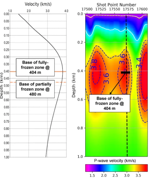
Hu et al. (2013) estimated the base of the fully frozen and partially frozen zones for all well-logging sites in the continental shelf of the CBS from borehole seismic velocity, electrical resistivity, and other well- logging geophysical data. The well-site, “IRKALUK B-35,” is located near shot point number 17,570 of our sur- vey line “ARA05C-L17” (see the map shown in Figure 4 and a bold black dot in Figure 8b). The distance between the well-site, “IRKALUK B-35”, and shot point number 17,570 of the line “ARA05C-L17” is less than 1 km. The results of the well-logging analysis for “IRKALUK B-35” extracted from Hu et al. (2013) are compared to the velocity profile obtained at shot point number 17,570 for survey line “ARA05C-L17.” The base of the fully frozen and partially frozen zones was estimated to be at 404 and 480 m depth, respectively, as shown in Figure 9. At the shot point number 17,570 in the inverted P-wave velocity model, reconstructed the P-wave velocity is around 3.8 km/s, which is the maximum value in this inverted model at the same depth of approximately 400 m. Also, the velocity contour of 3.6 km/s was reconstructed at around 500 m in this area (Figure 9). For comparing the results of the well-logging analysis, the minimum seismic velocity of the fully frozen and partially frozen zones can be determined as 3.8 and 3.6 km/s in the inverted seismic P-wave velocity model, respectively.
Figure 7. Initial and inverted P-wave velocity model for survey line “ARA05C-L05,” constructed by the LFWI method: (a) is the initial velocity model for applying LFWI (constant P-wave velocity of 3.0 km/s), and (b) is the inverted P-wave velocity model for MCS line “ARA05C-L05.” LFWI, laplace-domain full- waveform inversion; MCS, multichannel seismic.
6. Conclusions
This work is the first attempt to construct a two-dimensional P-wave velocity model for imaging the sub- sea permafrost and estimating the lower bound of these structures by applying the LFWI method to MCS data. The LFWI method allows reconstruction of the P-wave velocity model of subsea permafrost from seismic data even under challenging situations, such as shallow water depths of less than 50 m and ex- tremely high-velocity structures just beneath the seafloor. Inverted P-wave velocity models were verified and interpreted with previous results from the permafrost distribution map based on the seismic refrac- tion analysis, well-logging data, and a geothermal model. The inverted P-wave velocity models success- fully image the subsea permafrost structures, which were distributed with various sizes and shapes, and continuously characterize the lateral and vertical distributions of subsea permafrost on CBS in more detail than previous studies. Notably, the lower boundary of the subsea permafrost can be estimated using the velocity contours in the two-dimensional P-wave velocity models. We set the reference P-wave velocity for determining the lower bound of subsea permafrost in the P-wave velocity model, as 3.4 km/s refers to the depth of permafrost below the continental shelf of the CBS ranges from ∼100 to ∼600 m based on an analysis of geothermal modeling. The high-velocity structures with velocities greater than 3.4 km/s can be interpreted as the subsea permafrost structures with the ice content exceeding 40%, and these structures were distributed in the area where they belong to the discontinuous ice-bonded sediment area identified by Pullan et al. (1987). The estimated lower bound of subsea permafrost, according to our inverted models for most of the inner continental shelf, is around 650 m based on the lowest depth of the 3.4 km/s veloci- ty contours except several reconstructed high-velocity structures in the southernmost-east area. Also, the Figure 8. Initial and inverted P-wave velocity model for survey line “ARA05C-L17,” constructed by the LFWI method: (a) is the initial velocity model for applying LFWI (constant P-wave velocity of 3.0 km/s), and (b) is the inverted P-wave velocity model for MCS line “ARA05C-L17.” LFWI, Laplace-domain full- waveform inversion; MCS, multichannel seismic.
P-wave velocities of the fully and partially frozen zones of subsea permafrost structures can be estimated by our proposed velocity model as 3.8 km/s and 3.6 km/s, respectively, through comparison with the results of the well-logging analysis.
Data Availability Statement
The seismic data set used in this study and calculated P-wave velocity models by the Laplace domain full-waveform inversion from the seismic data set can be accessed online via the Korea Polar Data Center (KPDC) (https://dx.doi.org/doi:10.22663/KOPRI-KPDC-00001484.1).
References
Archer, D., Buffett, B., & Brovkin, V. (2009). Ocean methane hydrates as a slow tipping point in the global carbon cycle. Proceedings of the National Academy of Sciences of the United States of America, 106, 20596–20601. https://doi.org/10.1073/pnas.0800885105
Bae, H. S., Pyun, S., Shin, C., Marfurt, K. J., & Chung, W. (2012). Laplace-domain waveform inversion versus refraction-traveltime tomog- raphy. Geophysical Journal International, 190, 595–606. https://doi.org/10.1111/j.1365-246X.2012.05504.x
Brothers, L. L., Hart, P. E., & Ruppel, C. D. (2012). Minimum distribution of subsea ice-bearing permafrost on the U.S. Beaufort Sea conti- nental shelf. Geophysical Research Letters, 39, L15501. https://doi.org/10.1029/2012GL052222
Figure 9. Comparison of the results between the inverted P-wave velocity model by the LFWI algorithm and well- logging analysis: Velocity profile which was extracted from the inverted P-wave velocity model, and zoomed-in view of the inverted P-wave velocity model for survey line “ARA05C-L17” at the nearest point from the well-logging site
“IRKALUK B-35.” LFWI, Laplace-domain full-waveform inversion.
Acknowledgments
This work was supported by the re- search project entitled “Investigation of submarine resource environment and seabed methane release in the Arctic”
(KIMST, 20160247), which was funded by the Ministry of Oceans and Fisheries (MOF), Korea.
Brown, J., Ferrians, O. J., Jr., Heginbottom, J. A., & Melnikov, E. S. (Eds.), (1997). Circum-Arctic map of permafrost and ground-ice condi- tions. Washington, DC: U.S. Geological Survey.
Chadburn, S. E., Burke, E. J., Cox, P. M., Friedlingstein, P., Hugelius, G., & Westermann, S. (2017). An observation-based constraint on permafrost loss as a function of global warming. Nature Climate Change, 7, 340–344. https://doi.org/10.1038/nclimate3262
Ha, W., Cha, Y., & Shin, C. (2010). A comparison between laplace domain and frequency domain methods for inverting seismic waveforms.
Exploration Geophysics, 41, 189–197. https://doi.org/10.1071/EG09031
Ha, W., Chung, W., Park, E., & Shin, C. (2012). 2-D acoustic laplace-domain waveform inversion of marine field data. Geophysical Journal International, 190, 421–428. https://doi.org/10.1111/j.1365-246X.2012.05487.x
Ha, W., & Shin, C. (2012). Laplace-domain full-waveform inversion of seismic data lacking low-frequency information. Geophysics, 77, R199–R206. https://doi.org/10.1190/geo2011-0411.1
Hill, P. R., Mudie, P. J., Moran, K., & Blasco, S. M. (1985). A sea-level curve for the Canadian Beaufort shelf. Canadian Journal of Earth Sciences, 22, 1383–1393.
Hinz, K., Delisle, G., & Block, M. (1998). Seismic evidence for depth extent of permafrost in shelf sediments of the Laptev Sea, Rus- sian Arctic. Proceedings of the seventh international conference on permafrost (pp. 453–457). Yellowknife, NT: International Permafrost Association.
Hu, K., Issler, D. R., Chen, Z., & Brent, T. A. (2013). Permafrost investigation by well logs, and seismic velocity and repeated shallow temper- ature surveys, Beaufort-Mackenzie Basin (p. 33). Yukon, YT: Natural Resources Canada.
Hunter, J. A., Good, R. L., & Hobson, G. D. (1974). Mapping the occurrence of sub-seabottom permafrost in the Beaufort Sea by shallow refraction techniques (pp. 91–94). Ottawa: Geological Survey of Canada.
Hunter, J. A. M., Judge, A. S., MacAulay, H. A., Good, R. L., Gagne, R. M., & Burnes, R. A. (1976). Permafrost and frozen sub-seabottom materials in the southern Beaufort Sea. Victoria, BC: Beaufort Sea Technical Report 22.
Johansen, T. A., Digranes, P., van Schaack, M., & Lønne, I. (2003). Seismic mapping and modeling of near-surface sediments in polar areas.
Geophysics, 68, 1–8. https://doi.org/10.1190/1.1567226
Kang, S. G., Bae, H. S., & Shin, C. (2012). Laplace–Fourier-domain waveform inversion for fluid–solid media. Pure and Applied Geophysics, 169, 2165–2179. https://doi.org/10.1007/s00024-012-0467-7
Koo, N.-H., Shin, C., Min, D.-J., Park, K.-P., & Lee, H.-Y. (2011). Source estimation and direct wave reconstruction in Laplace-domain wave- form inversion for deep-sea seismic data. Geophysical Journal International, 187, 861–870. https://doi.org/10.1190/1.3513438 Kwon, J., Jin, H., Calandra, H., & Shin, C. (2017). Interrelation between Laplace constants and the gradient distortion effect in Laplace-do-
main waveform inversion. Geophysics, 82, R31–R47. https://doi.org/10.1190/geo2015-0670.1
Mackay, J. R. (1972). Offshore permafrost and ground ice, Southern Beaufort Sea, Canada. Canadian Journal of Earth Sciences, 9, 1550–1561.
Marfurt, K. J. (1984). Accuracy of finite-difference and finite-element modeling of the scalar and elastic wave equation. Geophysics, 49, 533–549.
Pullan, S. E., MacAuley, H. A., Hunter, J. A. M., Good, R. L., Gagne, R. M., & Burns, R. A. (1987). Permafrost distribution determined from seismic refraction. In B. R. Pelletier (Ed.), Marine Science Atlas of the Beaufort Sea: Geology and Geophysics/Atlas Des Sciences Marines De La Mer De Beaufort: Géologie Et Géophysique. Geological Survey of Canada, Miscellaneous Report 40, p. 37. https://doi.
org/10.4095/126967 (Open Access).
Pyun, S., Son, W., & Shin, C. (2011). Implementation of the Gauss Newton method for frequency-domain full waveform inversion using a logarithmic objective function. Journal of Seismic Exploration, 20, 193–206.
Rogers, J. C., & Morack, J. L. (1980). Geophysical evidence of shallow nearshore permafrost, Prudhoe Bay, Alaska. Journal of Geophysical Research, 85, 4845–4853. https://doi.org/10.1029/JB085iB09p04845
Ruppel, C. D. (2011). Methane hydrates and contemporary climate change. Nature Education Knowledge, 2, 12.
Shakhova, N., Semiletov, I., Leifer, I., Salyuk, A., Rekant, P., & Kosmach, D. (2010). Geochemical and geophysical evidence of methane release over the East Siberian Arctic shelf. Journal of Geophysical Research, 115, C08007. https://doi.org/10.1029/2009JC005602 Shin, C., & Cha, Y. H. (2008). Waveform inversion in the Laplace domain. Geophysical Journal International, 173, 922–931. https://doi.
org/10.1111/j.1365-246X.2008.03768.x
Shin, C., & Cha, Y. H. (2009). Waveform inversion in the Laplace–Fourier domain. Geophysical Journal International, 177, 1067–1079.
https://doi.org/10.1111/j.1365-246X.2009.04102.x
Shin, C., & Ha, W. (2008). A comparison between behavior of misfit functions for waveform inversion in the frequency and Laplace do- mains. Geophysics, 73, VE119–VE133. https://doi.org/10.1190/1.2953978
Shin, C., Koo, N.-H., Cha, Y. H., & Park, K.-P. (2010). Sequentially ordered single-frequency 2-D acoustic waveform inversion in the Lap- lace–Fourier domain. Geophysical Journal International, 181, 935–950. https://doi.org/10.1111/j.1365-246X.2010.04540.x
Shin, C., & Min, D.-J. (2006). Waveform inversion using a logarithmic wavefield. Geophysics, 71, R31–R42. https://doi.org/10.1190/1.2194523 Tarantola, A. (1984). Inversion of seismic reflection data in the acoustic approximation. Geophysics, 49, 1259–1266. https://doi.
org/10.1190/1.1441754
Taylor, A. E., Dallimore, S. R., Hill, P. R., Issler, D. R., Blasco, S., & Wright, F. (2013). Numerical model of the geothermal regime on the Beaufort shelf, arctic Canada since the Last Interglacial. Journal of Geophysical Research, 118, 2365–2379. https://doi.
org/10.1002/2013JF002859