Characterisation of an n-type segmented BEGe detector

Characterisation of an n-type segmented BEGe detector

1

I. Abt

, A. Caldwell

, B. Donmez

, C. Etrillard

, C. Gooch

, L. Hauertmann

, M.O. Lampert

,

2

H. Liao

, X. Liu

, H. Ma

, B. Majorovits

, O. Schulz

, M. Schuster

3

aMax-Planck-Institut f¨ur Physik, M¨unchen, Germany

4

bnow at University of Antalya, Turkey

5

cMirion France, Lingolsheim, France

6

dnow at Kansas State University, Manhattan, USA

7

eTsinghua University, Beijing, China

8

Abstract

9

A four-fold segmented n–type point-contact “Broad Energy” high-purity germanium detector, SegBEGe, has been characterised at the Max–Planck–Institut f¨ ur Physik in Munich. The main characteristics of the detector are described and first measurements concerning the detector prop- erties are presented. The possibility to use mirror pulses to determine source positions is discussed as well as charge losses observed close to the core contact.

Keywords: HPGe detectors, Position-sensitive devices, crystal axes, charge losses

10

1. Introduction

11

Germanium detectors are used in a wide variety of scientific applications [1], in fields like

12

medicine, homeland security and applied and fundamental physics [2–5]. “Broad Energy” Germa-

13

nium (BEGe) detectors have become increasingly important in searches for neutrinoless double

14

beta decay [6, 7]. The main challenge for these searches is the reduction of background. This

15

requires as perfect an understanding of the detector properties as possible.

16

The segmented n-type BEGe detector presented here was designed in order to study several

17

important features of BEGe detectors, which are of general interest but also connected to back-

18

ground suppression in searches for neutrinoless double beta decay. One interesting subject is the

19

influence of the crystal axes on the trajectories of the charge carriers and thus the pulse shapes.

20

This is linked to the mobility tensors of holes and electrons, which are not well known. The pulse

21

shapes are used by experiments such as GERDA [8] to identify Compton-scattering events which

22

accidentally deposit just the amount of energy expected for neutrinoless double beta decay. The

23

mirror pulses, as observed in segments which do not collect charge, are an important source of

24

information about the drifting charges inside the detector and provide spatial information. This

25

helps to understand and characterise the pulses.

26

The response of BEGe detectors to interactions close to the surface, where charge collection

27

inefficiencies are expected and not well understood, is another important issue. Of special interest

28

∗

is the area around the core contact. Charge losses on the surface can result in alpha surface

29

decays depositing the energy of neutrinoless double beta events. For this study, events close to

30

the surface were created with low energy gammas to study charge losses close to the core contact.

31

The charge losses can be identified using the characteristics of the mirror pulses. This allows the

32

characterisation of the pulses of the collecting electrode for such events.

33

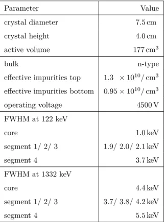
All results presented here were obtained from scans of the mantle and both end-plates of the

34

subject detector with a collimated

Barium source. The focus of this first characterisation were

35

events close to the surface from the 81 keV line of

Barium.

36

2. The Detector

37

The “SegBEGe” detector is an n-type high-purity Broad Energy Germanium (BEGe) detector,

38

segmented as depicted in Fig. 1. It has a diameter of 75 mm and a height of 40 mm. Its specifica-

39

tions as provided by the producer, Mirion France, formerly Canberra France, are listed in Table 1.

40

The side with the n

HV contact, i.e. the core contact, is called the top of the detector. The core

41

contact has a diameter of 15 mm and is surrounded by a passivated ring with an outer diameter

42

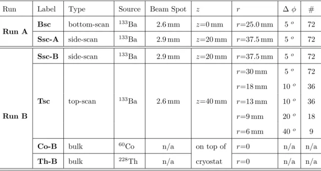
of 39 mm. The detector is four–fold segmented in φ with three individual 60-degree segments,

43

i=1,2,3, and one segment, segment 4, combining the three other regions in φ. Segment 4 is closed

44

on the bottom end-plate, see Fig. 1. The segmentation is created through a three-dimensional

45

implantation process. The center of the bottom plate is the origin of a cylindrical coordinate

46

system with the z-axis pointing towards the core contact. The left edge of segment 1, looking

47

from the top, defines φ = 0.

48

Figure 1: Schematics of the SegBEGe detector seen from the top (left) and from the bottom (right).

The electric field inside the detector is very similar to the field of an unsegmented detector. It

49

was calculated using an upgrade to the program package described in an earlier publication [9]. The

50

Parameter Value

crystal diameter 7.5 cm

crystal height 4.0 cm

active volume 177 cm

bulk n-type

effective impurities top 1.3 × 10

/ cm

effective impurities bottom 0.95 × 10

/ cm

operating voltage 4500 V

FWHM at 122 keV

core 1.0 keV

segment 1/ 2/ 3 1.9/ 2.0/ 2.1 keV

segment 4 3.7 keV

FWHM at 1332 keV

core 4.4 keV

segment 1/ 2/ 3 3.7/ 3.8/ 4.2 keV

segment 4 5.5 keV

Table 1: Specifications of the SegBEGe detector as provided by the manufacturer.

r ( ϕ = 270˚) r ( ϕ = 270˚)

Figure 2: Electric field strength (left) and potential (right) for ther−z cut through the detector atφ= 270^◦. Also shown are the field lines.

main improvements are the implementation of an adaptive grid and realistic segment boundaries.

51

The field distortions on the mantle close to the surface around the narrow segment boundaries

52

were found to be very shallow and insignificant for all gamma scans. The effect of the shape of the

53

segmentation on the bottom plate on the field lines is visible in Fig. 2 which shows the electrical

54

field strength and the potential as well as the field lines for the r − z cut through the detector at

55

φ = 270

. The slight asymmetry of the field lines seen around r = 0 is caused by the influence

56

of the inner boundary of segment 3. The “positive radii” in Fig. 2 indicate the cut through the

57

middle of segment 3, the “negative radii” indicate the cut through segment 4, which also covers

58

the centre of the bottom plate, see Fig. 1. Figure 2 is based on calculations where the width of

59

the floating segment boundaries was assumed to be 1 mm. This is not the precise width but shows

60

that the influence of the segment boundaries is small.

61

The potential close to the core contact of such a detector is high. It drops rapidly, creating a

62

strong field close to the core contact while the field close to the mantle of the detector is weak.

63

This causes the large differences in drift speed for different regions typical for this type of detector.

64

The field strength at the edges of the passivated ring around the HV contact is not expected

65

to be as high as indicated by the calculation. The calculation is based entirely on the boundary

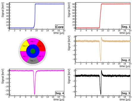
66

conditions for the potential which are 0 V for the segments, 4500 V for the core contact and

67

“floating” for the passivated ring. Neither the depth of the lithium drifted core contact nor the

68

lithium diffusion at the edge were implemented. Similarly, no depth or diffusion was implemented

69

for the boron implants of the segments. Especially, the diffusion is expected to reduce the spikes

70

in the field strength.

71

Figure 3: The experimental setup during a scan of the top of the detector during run B, figure taken from [10]. The cryostat is mounted on top of a liquid nitrogen dewar resting on a sandbag to reduce vibrations. Copper “ears” house the readout electronics. The source was positioned manually on a grid.

3. The Experimental Setup

72

The detector was mounted in a conventional aluminium vacuum-cryostat called K1 for the

73

characterisation measurements presented here. This cryostat was used previously to study the

74

performance of the first 18-fold segmented true coaxial detector [11]. Within K1, the detector

75

was cooled through a copper finger submerged in a conventional liquid nitrogen dewar. The

76

temperature at the top of the cooling finger was monitored using a PT100 inside the vacuum cap.

77

Between daily refilling, the temperature was stable between 102 K and 106 K. Any influence due to

78

changes in temperature was not corrected for in the studies presented here. The setup is depicted

79

in Fig. 3.

80

The signals were amplified by PSC 823 pre-amplifiers produced by Mirion France, which were

81

housed in the copper “ears” visible in Fig. 3. The DC-coupled room-temperature FETs for the

82

segment signals were mounted on the pre-amplifier boards in one of the ears. The cold FET for the

83

1G Ohms 1.2 nF

1G Ohms

0.8 pF

Output of the segments

Test input Drain Source

Feedback HV input

Full volume output

Pt100

Pt-100 output Inside Cryostat

JFET

Figure 4: Schematic of the detector readout, taken from [10]. The segment signals were processed in one ear and the core (full volume) signal in the other ear.

AC-coupled core signal was located inside the detector cap and was thermally coupled to the cold

84

finger. The rest of the core pre-amplification stage was located in the other ear. The schematic of

85

the readout is given in Fig. 4.

86

The detector was first mounted upside down, i.e. with the core contact down; this period is

87

called run A. For the following run B, the cryostat was opened and the detector was remounted with

88

the core contact up by the manufacturer. The data acquisition systems were different for runs A

89

and B. For run A, a PIXIE-4 system [12] with a 75 MHz sampling frequency and a 13.7 µs trace

90

length was used. This system used a trapezoidal filter for threshold triggering. It also provided

91

internal pile-up suppression. For run B, the system was upgraded with a Struck 16-channel

92

SIS3316-250-14 module [13]. This system provided a higher sampling frequency of 250 MHz and

93

a longer trace length of 20 µs. The latter is particularly important when pathologically long

94

pulses are expected. The Struck trigger can be programmed according to the requirements of the

95

measurement. A trapezoidal filter with additional constant fraction time-positioning for threshold

96

triggering was used. The system was not programmed to provide any online suppression of event

97

saturation or pile-up.

98

4. Data Taking

99

The detector was first commissioned in the fall of 2014. Run A lasted until summer 2015.

100

Run B, with the detector upright, lasted from March to April 2016.

101

Run Label Type Source Beam Spot z r ∆ φ # Run A

Bsc bottom-scan

Ba 2.6 mm z=0 mm r=25.0 mm 5

72

Ssc-A side-scan

Ba 2.9 mm z=20 mm r=37.5 mm 5

72

Run B

Ssc-B side-scan

Ba 2.9 mm z=20 mm r=37.5 mm 5

72

Tsc top-scan

Ba 2.6 mm z=40 mm

r=30 mm 5

72 r=18 mm 10

36 r=13 mm 10

36 r=9 mm 20

18 r=6 mm 40

9

Co-B bulk

Co n/a on top of r=0 n/a n/a

Th-B bulk

Th n/a cryostat r=0 n/a n/a

Table 2: Data sets used for this paper. The values listed under beam spot are the beam-spot radii on the detector surface. The z, andr values are nominal values listed in detector coordinates. The actual values varied slightly, see text. For side scans and top scans at different radii the number of scan points is given. The zand r values were controlled to

±0.5 mm,φwas controlled to±1 degree.

In both run periods, data were taken with an uncollimated

Cobalt and an uncollimated

102

228

Thorium source to illuminate the detector bulk and study resolutions. All detector scans were

103

performed with a

Barium source. The source was positioned manually to an accuracy of ≈ 2

104

in φ and ≈ 1 mm in r and z. The r-positioning setup is shown in Fig. 3. A similar setup was used

105

for side-scans.

106

Side-scans were performed in both runs. In run A (B), also the bottom (top) of the detector

107

was scanned. The data sets which were used for this paper are listed in Table 2. The table

108

uses detector coordinates; the scan coordinates for both runs were transformed into detector

109

coordinates. However, the r and z values are only nominal values. Due to a slight bend in the

110

cooling rod, the detector was not standing completely upright inside the cryostat [10]. Thus, z

111

was actually varying slightly during a side-scan. For top or bottom scans, r and φ were correlated

112

such that for an r scan φ varied slightly and vice versa. When individual beam-spot locations are

113

shown, the correct positions are indicated.

114

The gammas from the

Barium source were collimated with a 40 mm long tungsten collimator

115

with a diameter of 35 mm and a 1 mm radius collimation hole. A purely geometrical calculation

116

shows that for low energy gammas the beam spots on the detector surface were fully contained

117

within radii of 2.9 mm on the side and 2.6 mm on the end-plates. Considering the 1 mm radius

118

collimation, these beam spots are relatively large because the cryostat was originally designed to

119

hold a larger detector and thus there are gaps between the detector and the cryostat which are not

120

optimal. These beam spots are, however, sufficiently small to facilitate a first characterisation while

121

providing a signal-to-background ratio of typically better than 10 for the core and all segments

122

for all lines for single-segment events.

123

5. Data Processing

124

The online energy determination provided by the PIXIE system in run A was not used for the

125

results presented here. However, the PIXIE system suppressed pile-up and saturated events online

126

while the Struck system was not programmed to suppress such events. For run B, events from

127

pile-up and saturation were suppressed by evaluating the slopes of the baseline and the decay-

128

corrected signal plateau. A negative baseline slope indicates pile-up and a positive plateau slope

129

indicates saturation. During barium scans, a total of about 5 % of the events were rejected. These

130

were dominated by events with a saturated amplifier. Actual pile-up was at the level of about 1 %.

131

The rest of the offline data processing was identical for both runs. The recorded raw pulses were

132

baseline subtracted and corrected for the pre-amplifier specific decay of the pulses [10, 14]. Signal

133

amplitudes were derived using a fixed-size window filter, where the position of the window was

134

determined by the trigger. For run A (B), a baseline window of 4.48 µs (8.0 µs) and an amplitude

135

window of 6.63 µs (9.0 µs) were chosen. This filter introduces the least bias with respect to different

136

pulse shapes. The baseline and amplitude windows were separated far enough to ensure that the

137

actual rise of the pulse started after the baseline and ended before the amplitude window.

138

Cross-talk effects between the core and the segments as well as between segments were treated

139

in an automated calibration procedure using single-segment events [10, 14]. A calibration was

140

performed for each data set individually. The cross-talk correction was performed under the

141

assumption that the cross-talk from all segments to the core was identical. This assumption

142

affected the core energy scale for single-segment events in different segments by less than 0.1 % [10,

143

14]. In effect, this lowers the core energy resolution, but the impact is negligible. The cross-talk

144

from one particular segment to another segment is always measured together with the cross-talk

145

from the core to this segment. Segment 4 events resulted in a cross-talk of 1 ∼ 2 % into the small

146

segments 1,2 and 3 while events in these small segments caused a cross-talk of about 0.4 % into

147

the large segment 4.

148

6. Overall Detector Performance

149

The detector performed as expected in the K1 cryostat. The conditions in this setup were

150

not perfect with respect to grounding and shielding. Thus, the resolutions were slightly lower

151

Energy [keV]

0 500 1000 1500 2000 2500 3000

Counts / keV

1 10 102

103

104

Figure 5: Core spectrum from a 1-hourTh-Bdata set.

FWHM [keV]

Source γ-line [keV] Core Seg. 1 Seg. 2 Seg. 3 Seg. 4

133

Ba

81 3.29 5.15 4.05 4.07 7.26

356 2.64 4.58 3.47 3.52 6.04

60

Co 1173 4.57 4.88 4.16 4.34 8.05

1332 4.93 5.00 4.39 4.14 7.84

228

Th 2614 7.65

Table 3: Energy resolutions as absolute FWHMs in keV for the core and all segments as observed in run B.

than listed by the manufacturer. Results from run B are listed in Table 3. The lack of energy

152

dependence for the resolutions demonstrates that the results are dominated by electronic noise.

153

However, the detector resolution did not affect any of the results presented here. The main purpose

154

of this setup was to characterise such a detector. If such a detector were to be deployed in an

155

actual experiment, a completely different electronics setup with the pre-amplification closer to the

156

detector would be chosen.

157

Figure 5 shows the core spectrum for a 1-hour Th-B data set. The 2614 keV

Tl line is clearly

158

visible as well as the

Bi lines at 239 and 1620 keV. In addition, the natural background in the

159

laboratory features the usual lines from the uranium decay chain as well as a strong 1460 keV line

160

from

K.

161

The double-escape peak from the 2614 keV thallium line at 1592 keV and the 1620 keV bismuth

162

line were used for a standard pulse-shape analysis to show that the segmentation did not affect the

163

core pulses. The bismuth line is dominated by multi-site events from Compton scattering. The

164

double-escape peak is dominated by single-site events; in these events all the energy is deposited in

165

one small volume. The so-called A/E-method uses as a discriminator the ratio of A, the maximum

166

of the first derivative of a pulse, i.e. the maximum current, divided by the total energy of the event.

167

The method was applied to Th-B data [10]. For a survival probability of the double-escape peak

168

of 90 %, a reduction of the bismuth peak of 86 % was obtained. That is compatible with the results

169

obtained for other BEGe detectors [6, 15].

170

7. Super-pulses

171

µs]

time [

0 2 4 6 8 10 12 14 16 18 20

Signal [keV]

−20 0 20 40 60 80 100

Core

µs]

time [

0 2 4 6 8 10 12 14 16 18 20

Signal [keV]

−40

−20 0 20 40 60 80 100

Seg. 1

µs]

time [

0 2 4 6 8 10 12 14 16 18 20

Signal [keV]

−30

−20

−10 0 10 20 30

Seg. 2

µs]

time [

0 2 4 6 8 10 12 14 16 18 20

Signal [keV]

−5040

−30

−20

−10

−0 10 20 30 40

Seg. 4

µs]

time [

0 2 4 6 8 10 12 14 16 18 20

Signal [keV]

−30

−20

−10 0 10 20 30

Seg. 3

Figure 6: Single 81 keV event from theSsc-Bdata set forφ= 45^◦. The core pulse is shown at the top left, segments 1,2,3 are shown from top to bottom on the right and segment 4 is shown at the bottom left. The inset depicts the detector top with aφscale.

The 81 keV line from

Ba was chosen as the line for which scanning results are presented.

172

The gammas from this line have a penetration depth of about 1.8 mm and thus create events very

173

close to the surface. As a result, the holes are collected quickly and the drift is dominated by

174

electrons. A single event at 81 keV as recorded in the Ssc-B data set at φ = 45

is shown in Fig. 6.

175

The event was located on the surface of segment 1. The largest mirror pulse is expected in

176

segment 4 next to the collecting segment 1. It is clearly visible in Fig. 6. Smaller mirror pulses

177

are expected in segments 2 and 3. The noise level is such that they cannot be easily identified in

178

individual events.

179

The pulses induced by low energy gammas, such as from the 81 keV line, are all very similar due

180

to their low penetration power. Thus, they can be averaged to form super-pulses. The selection

181

of events to contribute to a super-pulse was:

182

µs]

time [

0 2 4 6 8 10 12 14 16 18 20

Signal [keV]

0 10 20 30 40 50 60 70 80

Core

µs]

time [

0 2 4 6 8 10 12 14 16 18 20

Signal [keV]

0 10 20 30 40 50 60 70 80

Seg. 1

µs]

time [

0 2 4 6 8 10 12 14 16 18 20

Signal [keV]

−8

−6

−4

−2 0 2

Seg. 2

µs]

time [

0 2 4 6 8 10 12 14 16 18 20

Signal [keV]

−30

−25

−20

−15

−10

−5 0

Seg. 4

µs]

time [

0 2 4 6 8 10 12 14 16 18 20

Signal [keV]

−6

−4

−2 0 2

Seg. 3

Figure 7: Super-pulse for 81 keV events from the Ssc-Bdata set for φ= 45^◦. The core super-pulse is shown at the top left, segments 1,2,3 are shown from top to bottom on the right and segment 4 is shown at the bottom left. Please note the different scales used for the different segments. The inset depicts the detector top with aφscale.

• After calibration and cross-talk correction, all events, for which the segment under investiga-

183

tion, i, registered an energy within 10 keV of the core energy, were flagged as single-segment-i

184

events;

185

• If the energy of the core was within 3 sigma of a known

Ba photon line (the sigma for

186

each was determined by fitting a Gaussian to the core energy spectrum) an event got flagged

187

as belonging to that line;

188

• There was no offline alignment needed because the trigger procedure of the DAQ already

189

aligned the core pulses.

190

The pulses from the events which were selected this way were averaged. This is only reasonable

191

for low-energy lines because at higher energies, the spread of interaction points is too large. The

192

studies presented in this paper focus on the 81 keV line, for which the procedure is reasonable.

193

The signal-to-background ratio for 81 keV single-segment-i events was around 10 for i = 4 and

194

higher for the other segments. Therefore, there was, unless mentioned otherwise, no rejection

195

of background events, which are mainly due to Compton scatters. These background events are

196

deeper in the bulk and have lower rise-times. When averaged in, they cause the super-pulse to

197

have a slightly lower rise-time. This mostly affects segment 4 which has a higher background level

198

due to its larger volume. For the future, it is planned to have a pre-selection using the quality of

199

fits to Monte Carlo surface pulses [9].

200

Typically, 2000 to 2500 pulses were averaged. The super-pulse for the location of the event

201

depicted in Fig. 6 is shown in Fig. 7. The super-pulse also clearly reveals the smaller mirror pulses

202

in segments 2 and 3. As the noise gets averaged out super-pulses are a powerful tool to investigate

203

detector properties.

204

8. Segment Boundaries

205

°] φ [

0 50 100 150 200 250 300 350

ssi/allCore: R

0 0.2 0.4 0.6 0.8

1 Tsc, r=30mm Ssc-B Ssc-A Bsc

i = 1 i = 2 i = 3

°] φ [

0 50 100 150 200 250 300 350

ss4/allCore: R

0 0.2 0.4 0.6 0.8 1

Figure 8: RatiosRss_i/all for (top) the three individual segments i=1,2,3 and (bottom) the large segment 4. Shown are data for run A (open symbols) and run B (full symbols). Also shown are fits of the function in Eq. 1 to theTscdata from run B.

The segment boundaries were determined using the rate of single-segment events in the re-

206

spective bottom-, side- and top-scans. The ratios, R

, of the number of single-segment events

207

in segment i with i ∈ [1, 2, 3, 4] over all single-segment events were used. A value close to one is

208

expected if the source is facing the respective segment, close to zero, depending on the background

209

level, is expected otherwise. The data as obtained for the 81 keV line from

Ba in the Bsc, Ssc-

210

A/B and Tsc scans are depicted in Fig. 8. Segment 4 has a higher background level due to its

211

larger volume. The side-scans were affected by some parts of the detector holder, reducing the

212

event numbers in the middle of some segments. Also shown are the results of fits to the Tsc data

213

using the function:

214

R

(φ) = H

2 · tanh[Λ · (φ − φ

)] + Γ , (1) where the four fitted parameters are

215

• H : the maximal variation in R

,

216

• Λ: the slope of the variation in R

: Λ > (<) 0 for rising (falling) edges,

217

• φ

: the boundary between segments i and j,

218

• Γ: the source location independent background.

219

The segment boundaries were found consistently in all scans during both run periods. The

220

information was mainly used to have precise location information on the detector.

221

9. Crystal Axes

222

° ] φ [

0 50 100 150 200 250 300 350

[ns]

t

350 400 450 500 550

1 4 2 4 3 4

Tsc, r = 30mm Bsc

° ] φ [

0 50 100 150 200 250 300 350

[ns]

t

350 400 450 500 550

1 4 2 4 3 4

Ssc-B Ssc-A

Figure 9: Average 5 % to 95 % rise-times of 81 keV super-pulses as a function of the azimuth angleφfor (bottom) the two side-scans from runs A and B and (top) the bottom-scan at r= 25 mm and the top-scan atr= 30 mm from runs A and B, respectively. The error bars represent an uncertainty corresponding to a temperature shift of roughly 2 K.

The propagation of electrons and holes in the electric field of the germanium crystal is influenced

223

by the crystal axes [16, 17]. The charge carriers get deflected and do not follow simple radial paths.

224

Thus, the time to collect the charge carriers depends on the angle between the closest crystal axis

225

and the radial line on which the interaction takes place. The dependence of the resulting rise-time

226

versus φ is usually analytically described by a sine function:

227

t

= C + a · sin 2π

90 (φ + φ

)

, (2)

where t

is the time a pulse needs to rise from 5 % to 95 % of its amplitude, C is the mean

228

t

and a the amplitude of the variation of t

. The parameter φ

is fitted to determine

229

the location of the axes.

230

The data using 81 keV super-pulses are shown in Fig. 9 for scan data from both run A and B.

231

The error bars shown in Fig. 9 represent the uncertainty due to changes in the temperature, which

232

was not controlled to better than ± 2 K. The data from the different periods and scans agree

233

reasonably well. However, the scan data were affected by the small tilt of the detector that caused

234

shifts of the impact points with respect to the nominal detector coordinates. This effect was not

235

corrected for. The top-scan was affected more than the bottom-scan because the difference in

236

drift paths for slight variations in r is larger for the top than the bottom surface, see Fig. 2.

237

There are some discontinuities visible at edges of segment 4, where the rise-times in segment 4 are

238

lower than in the neighbouring segment. This is due to the higher background level in segment 4.

239

The background events are located deeper in the bulk and have shorter rise-times. This distorts

240

the super-pulses slightly. The effect is too small to affect the determination of the crystal axes

241

significantly.

242

° ] φ [

0 50 100 150 200 250 300 350

[ns]

t

380 390 400 410 420 430 440 450 460 470 480

Ssc-A Fit Χ2

Figure 10: Average 5 % to 95 % rise-times of 81 keV super-pulses from Ssc-A together with a fit according to Eq. 2.

The side-scan data from run A are shown together with a fit according to Eq. 2 in Fig. 10. The

243

sine function describes the data well. The φ values for which the drift-time is maximal indicate

244

the so-called “slow axes”. The axes with minimal drift-time are called “fast axes”. The difference

245

between drift-times will, in the future, be compared to simulation results to study the mobility of

246

electrons.

247

10. Position Reconstruction

248

The electrons and holes drifting to the electrodes of the collecting segment create mirror charges

249

in the neighboring segments. These mirror pulses end at the baseline once the charge carriers

250

are collected at the electrodes. This phenomenon can be understood and deduced from Ramo’s

251

theorem.

252

µs]

Time [

7.5 8 8.5 9 9.5 10 10.5 11

Norm. Induced Charge

−0.2

−0.15

−0.1

−0.05 0

Phi 60.7 Phi 65.9 Phi 70.9 Phi 76.0 Phi 81.0 Phi 86.0

Phi 90.9 Phi 95.8 Phi 100.6 Phi 105.5 Phi 110.3 Phi 115.0

µs]

Time [

7.5 8 8.5 9 9.5 10 10.5 11

Norm. Induced Charge ⁰ 0.2 0.4 0.6 0.8

1 Phi 60.7

Phi 65.9 Phi 70.9 Phi 76.0 Phi 81.0 Phi 86.0

Phi 90.9 Phi 95.8 Phi 100.6 Phi 105.5 Phi 110.3 Phi 115.0

µs]

Time [

7.5 8 8.5 9 9.5 10 10.5 11

Norm. Induced Charge

−0.2

−0.15

−0.1

−0.05 0

Phi 60.7 Phi 65.9 Phi 70.9 Phi 76.0 Phi 81.0 Phi 86.0

Phi 90.9 Phi 95.8 Phi 100.6 Phi 105.5 Phi 110.3 Phi 115.0

segment 1

segment 4

segment 2

Figure 11: From top to bottom: The super-pulses in segments 1, 4, 2 from the data set Ssc-Bin the range 60^o < φ <120^o for the 81 keV line, adapted from [10]. All pulses are normalised to an amplitude of 1 in the collecting segment 4.

The super-pulses from the 81 keV line for 60

< φ < 120

from the Ssc-B data set are shown

253

in Fig. 11 for the segments 1, 4, 2. The shape of the mirror pulses observed in segments 1 and 2

254

depends on the location of the energy deposit. The mirror pulses reflect the different drift-paths

255

of the charge carriers. The maximum of the absolute amplitude, M A

with i = 1, 2, depends on

256

the closest approach of the charge carriers to the segment-i electrode.

257

The mirror pulses are all negative because only the drift of the electrons is seen. The M A

258

values decrease as the source moves away towards segment 2. At the same time the M A

values

259

°] φ [

60 70 80 90 100 110 120

Norm. Mirror Pulse Amplitude

−0.24

−0.22

−0.2

−0.18

−0.16

−0.14

−0.12

−0.1

Seg. 1 mirror pulse Seg. 2 mirror pulse Slow crystal axis Seg. 4 center

°] φ [

60 70 80 90 100 110 120

Norm. Mirror Pulse Amplitude

−0.24

−0.22

−0.2

−0.18

−0.16

−0.14

−0.12

−0.1

−0.08

Seg. 1 mirror pulse Seg. 2 mirror pulse Slow crystal axis Seg. 4 center

Figure 12: The mirror pulse amplitudes of the¹³³Ba 81 keV super-pulses for theSsc-B(left) and Tsc (right) scans for the area of segment 4 between segment 1 and segment 2. Also indicated are the segment boundaries (solid vertical lines), the centre of segment 4 (dotted vertical line) and the location of the slow axis (dashed-dotted vertical line). The data points are connected with straight lines to guide the eye.

°] φ [

60 70 80 90 100 110 120

α

−0.4

−0.3

−0.2

−0.1 0 0.1 0.2 0.3

0.4 Seg. 4 center

Slow crystal axis

+ MA2 MA1

- MA2 MA1 α = Linear Fit Slope: -0.013 Ordinate: 1.173

°] φ [

60 70 80 90 100 110 120

α

−0.4

−0.2 0 0.2 0.4

Seg. 4 center Slow crystal axis

+ MA2 MA1

- MA2 MA1 α = Linear Fit Slope: -0.016 Ordinate: 1.429

Figure 13: The asymmetries of mirror pulse amplitudes of the super-pulses for theSsc-B (left) andTsc (right) scans for the area of segment 4 between segment 1 and segment 2.

Also shown are linear fits to the data.

increase. Both segments also show that not only the amplitude of the mirror pulse changes but

260

also the time at which the amplitude is reached. The pulse in the collecting segment 4 only changes

261

moderately. This moderate change is due to the influence of the slow axis which is contained in

262

that sector of segment 4.

263

The amplitudes, M A

and M A

, of the pulses depicted in Fig. 11 are shown in the left panel

264

of Fig. 12. The right panel depicts equivalent data from the top-scan Tsc. Also indicated in the

265

figure are the segment boundaries, the centre of segment 4 and the location of the slow axis. Due

266

to the influence of the slow axis, the cross-over point between the two segment amplitudes is not

267

at the segment centre. Trajectories are bent towards the slow axis and thus the cross-over point

268

is pulled towards the slow axis. The effect is larger for the Tsc data because from z = 40 mm and

269

r = 30 mm the inwards drift affected by the slow axis passes through a relatively low field a bit

270

longer than for the Ssc-B data at z = 20 mm and r = 37.5 mm.

271

In order to reconstruct the position of the source, a simple asymmetry, α, was used:

272

α = M A

− M A

M A

+ M A

. (3)

The asymmetries for the mirror pulse amplitudes together with linear fits are shown in Fig. 13.

273

There was no attempt made to provide statistical or a priori systematical uncertainties. The

274

linear fits are quite good. However, they provide different slopes and ordinates. The charge

275

carrier trajectories are very different for side and top-scans. Considering this, the differences are

276

expected. In general, the trajectories are very dependent on the z-position for side-scans and

277

r-position for top-scans. Thus, a simple asymmetry like α can only reconstruct the φ of surface

278

events to about 10 degrees [10] if there is no information on z (r) available.

279

11. Charge Losses around the Core Contact

280

The core contact and the surrounding passivation ring were investigated especially to look for

281

possible charge losses. The core spectra for selected scan points at different radii are shown in

282

Fig. 14. There was no selection using core or segment energies.

283

The core spectra show marked differences depending on the location of the beam spot. The

284

effect on individual peaks depends on their energy, i.e. on the penetration depth of the gammas:

285

• The double peak at 31 keV and 35 keV from the

Ba source is nicely resolved for the

286

reference point at r = 32 mm. As the beam spot moved inwards hitting the passivation area,

287

the observed energy was reduced and the resolution to resolve the double peak was lost.

288

This is compatible with a layer underneath the passivation, where some of the deposited

289

charge cannot be collected. When the beam spot illuminated the core contact, these low

290

energy gammas could not be observed. This is compatible with the expectation for a Lithium

291

drifted core contact creating an inactive volume of about 1 mm depth.

292

• The 81 keV peak developed a secondary peak as soon as the passivation area was reached

293

at r = 18 mm. At that position, some events still showed the full energy. This was either

294

due to the beam spot touching the regular area of the detector or due to the inactive layer

295

being thin enough such that some gammas could penetrate deep enough. At r = 13 mm

296

and r = 9 mm, only a broader peak with reduced energy was observed. This indicates a

297

relatively regular layer where about 10 keV are lost. When the beam spot reached the core

298

contact, some gammas penetrated deep such that the full energy could be observed.

299

Energy [keV]

0 50 100 150 200 250 300 350 400

Counts / keV

1 10 102 103 104

Energy [keV]

0 10 20 30 40 50 60 70 80 90 100

Counts / keV

1 10 102 103 104

Seg. 2 Seg. 1

Seg. 3 Seg. 4

Seg. 4

Seg. 4

Core Spectrum for radii, r:

regular: r = 32mm passivation: r = 18mm passivation: r = 13mm passivation: r = 9mm contact area: r = 6mm

Figure 14: The core spectra for a radial top-scan with the collimated¹³³Ba source, adapted from [10]. The beam spots are indicated on the bottom left. They illuminated areas from the “regular” area of the detector inwards to the passivated ring and the core contact. The spectra are shown from 10 to 400 keV in the top left and from 10 to 100 keV in the top right.

The spectra are coloured (shaded) according to the legend.

• The higher energy lines show pronounced low-energy shoulders which are caused by events

300

with a shallow interaction point, for which some energy is lost. For most events the expected

301

energy is recorded.

302

In summary, the observations are compatible with the expected inactive volume of the core contact

303

and a layer underneath the passivation ring where charge can also not be collected.

304

The behaviour as shown in Fig. 14 was the same for a given r, independent of φ. Information

305

from the segments were used to further investigate the effect. A radial scan in the middle of

306

segment 3 was chosen. Figure 15 provides information on the segment and core energies for

307

individual events for a beam spot on the outer edge of the passivation ring.

308

Even though gammas in the beam spot deposited their energy very close to segment 3, all

309

segments show events where the charge is actually collected in these segments. For these events,

310

[keV]

ECore 20 30 40 50 60 70 80 90 100 core / ESeg1E

−0.2 0 0.2 0.4 0.6 0.8 1 1.2

0 2 4 6 8 10 12 14 16 18 20 22 24

[keV]

ECore 20 30 40 50 60 70 80 90 100 core / ESeg2E

−0.2 0 0.2 0.4 0.6 0.8 1 1.2

0 5 10 15 20 25 30

[keV]

ECore 20 30 40 50 60 70 80 90 100 [keV]Core - ESegSumE

−20

−15

−10

−5 0 5 10 15 20

0 1 2 3 4 5 6 7 8 9 10

° = 267 φ Radius = 18mm;

Source facing Seg. 3

[keV]

ECore 20 30 40 50 60 70 80 90 100 core / ESeg3E

−0.2 0 0.2 0.4 0.6 0.8 1 1.2

0 2 4 6 8 10 12 14 16 18

[keV]

ECore 20 30 40 50 60 70 80 90 100 core / ESeg4E

−0.2 0 0.2 0.4 0.6 0.8 1 1.2

0 2 4 6 8 10 12 14 16 18 20

Seg. 2 Seg. 1

Seg. 3 Seg. 4

Seg. 4

Seg. 4

Figure 15: Distributions of the ratios of segment energies,E_{Seg i}, divided by the core energy Ecorevs.Ecorefori= 1 to 4 in the four left panels. The top right panel shows the difference between

P

ESeg iandEcorevs. Ecore. The graphic at the bottom right indicates the source position on the passivated area. The boxes around clusters for segments 3 and 4 indicate selections to form super-pulses.

the segment- to core-energy ratio R

= E

/E

≈ 1. For segments 1 and 2, they are associated

311

with background; there are no clusters with R

≈ 1, observed at the core energy peaks between

312

20 keV and 30 keV and between 70 keV and 80 keV. The expected clusters with R

≈ 0 are clearly

313

visible.

314

For segment 3, a small cluster with R

≈ 1 is observed for the 81 keV line. Most of the events,

315

however, are clustered around a reduced core energy and a ratio of R

≈ 0.7. This is true for the

316

31/35 keV double-peak and the 81 keV peak. Segment 4 seems to reestablish the energy balance

317

by collecting almost all of the charges missing in segment 3. If the energies as measured in all

318

segments were added, the energy balance was indeed recovered as also shown in Fig. 15.

319

In order to clarify the situation, the events attributed to the 81 keV photon line and marked by

320

boxes in Fig. 15 were used to form super-pulses for the core and all segments for this beam-spot

321

location. The core energy has to be within 3 sigma of photon-line energy as fitted in the core

322

spectrum. The cut on the ratios R

and R

was selected by eye. The pulses were normalised

323

to the core energy before averaging. The result is shown in Fig. 16 together with results for three

324

more beam spot locations, for which similar selections were performed. These selections ensure

325

Time [ns]

8500 9000 9500 10000 10500 11000 11500 12000 12500 13000

Normalized Induced Charge

0 0.2 0.4 0.6 0.8

1Core

Mean Energy [keV]:

r = 18mm: 72.83 r = 13mm: 72.03 r = 9mm: 72.90 r = 6mm: 73.55

Time [ns]

8500 9000 9500 10000 10500 11000 11500 12000 12500 13000

Normalized Induced Charge

−0.05 0 0.05 0.1 0.15 0.2

Seg. 1

Seg. 2 Seg. 1

Seg. 3 Seg. 4

Seg. 4

Seg. 4

Time [ns]

8500 9000 9500 10000 10500 11000 11500 12000 12500 13000

Normalized Induced Charge

−0.05 0 0.05 0.1 0.15 0.2

Seg. 2

Time [ns]

8500 9000 9500 10000 10500 11000 11500 12000 12500 13000

Normalized Induced Charge

0 0.2 0.4 0.6 0.8

1Seg. 4

Time [ns]

8500 9000 9500 10000 10500 11000 11500 12000 12500 13000

Normalized Induced Charge

0 0.2 0.4 0.6 0.8

1Seg. 3

Figure 16: Super-pulses for 81 keV events as indicated by the small boxes in Fig. 15. The top left panel depicts core pulses, segments 1 to 3 are shown from top to bottom on the right, segment 4 pulses are depicted on the bottom left. The scale is a factor 5 smaller for segments 1 and 2. The graphic at the centre left indicates the source positions. Source positions and line appearance are matched in colour (shading).

that only events where segment 3 acts as the main collecting segment contribute to the super-

326

pulses. Due to the tilt discussed earlier, the azimuth angle φ changed as the radius was reduced.

327

This results in the innermost beam-spot location being shifted in front of segment 4. For this

328

beam-spot location, events collected in segment 4 were selected according to the boxes in Fig. 17.

329

The super-pulses in Fig. 16 provide information on what happened to the charge carriers in the

330

events. For all four locations, segments 1 and 2 show mirror pulses. They are not collecting. For

331

the three outer points, segment 3 collects most of the charge, but segment 4 also collects charge.

332

For the innermost point, segment 4 collects the charge and segment 3 shows a mirror pulse. All

333

mirror pulses shown do not return to the baseline. This indicates charge trapping.

334

For r = 18 mm, the mirror pulses in segments 1 and 2 are at first negative, i.e. dominated by

335

electrons. They turn positive after about 200 ns, indicating that holes are still not collected. This

336

is confirmed by the pulses in the collecting segments 3 and 4 which flatten out around 9500 ns and

337