RESEARCH ARTICLE
10.1002/2016MS000650
Designing variable ocean model resolution based on the observed ocean variability
Dmitry V. Sein1,2, Sergey Danilov1,3, Arne Biastoch4, Jonathan V. Durgadoo4, Dmitry Sidorenko1, Sven Harig1, and Qiang Wang1
1Alfred Wegener Institute, Helmholtz Centre for Polar and Marine Research, Bremerhaven, Germany,2P. P. Shirshov Institute of Oceanology RAS, St.Petersburg, Russia,3A. M. Obukhov Institute of Atmospheric Physics RAS, Moscow, Russia,
4GEOMAR Helmholtz Centre for Ocean Research Kiel, Kiel, Germany
Abstract
If unstructured meshes are refined to locally represent eddy dynamics in ocean circulation models, a practical question arises on how to vary the resolution and where to deploy the refinement. We propose to use the observed sea surface height variability as the refinement criterion. We explore the utility of this method (i) in a suite of idealized experiments simulating a wind-driven double gyre flow in a strati- fied circular basin and (ii) in simulations of global ocean circulation performed with FESOM. Two practical approaches of mesh refinement are compared. In the first approach the uniform refinement is confined within the areas where the observed variability exceeds a given threshold. In the second one the refinement varies linearly following the observed variability. The resolution is fixed in time. For the double gyre case it is shown that the variability obtained in a high-resolution reference run can be well captured on variable- resolution meshes if they are refined where the variability is high and additionally upstream the jet separa- tion point. The second approach of mesh refinement proves to be more beneficial in terms of improvement downstream the midlatitude jet. Similarly, in global ocean simulations the mesh refinement based on the observed variability helps the model to simulate high variability at correct locations. The refinement also leads to a reduced bias in the upper-ocean temperature.1. Introduction
Although eddy-resolving ocean climate models are already feasible in climate studies [Griffies et al., 2015], they still require a considerable computational effort, and currently most climate simulations are done with eddy-permitting or coarser ocean models. It is expected that resolving small-scale dynamics in certain areas may improve the representation of the large scale circulation, as is for example the case for coastal upwell- ing systems [see e.g.,Small et al., 2015]. There are many other places in the ocean where local mesh refine- ment may contribute to increase model fidelity through increased realism in rendering topography and coastlines, reduced dissipation, or better representation of meso-scale processes such as lateral spreading or eddy fluxes. Learning about the impact of locally resolved dynamics on the general ocean circulation motivates a growing number of studies which use models formulated on nested or generalized curvilinear meshes to locally resolve eddy dynamics in regions of interest [see e. g.,Durgadoo et al., 2013;Kawasaki and Hasumi, 2014;Talandier et al., 2014;Sein et al., 2015]. In these cases globally relevant regional dynamics can be simulated at a moderate computational cost compared to running a global eddy resolving model.
Models based on unstructured meshes, such as the Finite-Element Sea-ice Ocean Model (FESOM) [Wang et al., 2014] and MPAS-ocean [Ringler et al., 2013], provide an alternative option for multiresolution ocean simulations. Although they are still not common in ocean climate modeling, they became mature and are already practically used in climate studies [Sidorenko et al., 2015]. Compared to traditional nested models or models with generalized curvilinear meshes, unstructured-mesh models offer more flexibility for imple- menting locally refined resolution. Their refined areas can be of arbitrary shape and their resolution can be varied according to the desired function. However, the question of how to select this function remains a research topic because we want to achieve expected improvement in simulated results with decrease or least increase in computational cost. Furthermore, there are intrinsic limitations in practice, for the proximity of coarse and fine meshes implies a certain effective damping for the dynamics on the fine mesh [Danilov and Wang, 2015].
Key Points:
Observed sea surface hight variance was used as a critarion for mesh refinement in ocean model
Presented approach improves the representation of eddy variability and ocean hydrography
Correspondence to:
D. V. Sein, Dmitry.Sein@awi.de
Citation:
Sein, D. V., S. Danilov, A. Biastoch, J. V. Durgadoo, D. Sidorenko, S. Harig, and Q. Wang (2016), Designing variable ocean model resolution based on the observed ocean variability,J.
Adv. Model. Earth Syst.,8, 904–916, doi:10.1002/2016MS000650.
Received 15 FEB 2016 Accepted 12 MAY 2016
Accepted article online 17 MAY 2016 Published online 4 JUN 2016
VC2016. The Authors.
This is an open access article under the terms of the Creative Commons Attribution-NonCommercial-NoDerivs License, which permits use and distribution in any medium, provided the original work is properly cited, the use is non-commercial and no modifications or adaptations are made.
Journal of Advances in Modeling Earth Systems
PUBLICATIONS
It is commonly assumed that the local Rossby deformation radius has to be resolved with several grid cells in order to simulate mesoscale eddies, for one has to represent dynamics related to the development of baroclinic instability. The Rossby radius is known to vary in a wide range, from 50 to 30 km at midlatitudes to less than 10 km in high latitudes, especially on high-latitude continental shelves [seeHallberg, 2013, Fig- ure 1] for a map of resolution needed to resolve the first baroclinic Rossby radius with two mesh intervals).
Resolution in global models using Mercator grids follows the latitudinal changes in Rossby radius to some extent, but the setups that would be eddy resolving in high latitudes are computationally demanding.
Unstructured meshes can certainly be designed to exactly follow the scale of the first baroclinic Rossby radius, with resolution more optimally distributed than on structured meshes. Although feasible in principle, such meshes are still too large in size and may be suboptimal in practical ocean climate simulations because of the model time step limitation on smallest grid cells related to mesh nonuniformity.
A simpler mesh refinement approach is to follow the idea of traditional nesting, and use the unstructured- mesh functionality to provide locally uniformly refined patches within a relatively coarse global mesh. The positive side of this approach is mesh uniformity over fine patches, hence certain uniformity in terms of the grid-cell Reynolds number (note that it may still vary depending on parameterizations used). A drawback is that fine resolution is just used to cover one or a few selected areas without accounting for the fact that the mesoscale eddy activity in the real ocean is far from being uniform in space.
In this work we propose a new way to configure variable mesh resolution for unstructured-mesh models.
We use observed sea surface height variability (SSHV) to decide whether mesh resolution needs to be refined or not. The SSHV is defined as the standard deviation of sea surface height, which can be considered
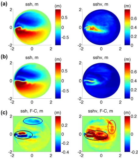
Figure 1.Mean (left) SSH and (right) SSHV in reference simulations on the (top) fine mesh, (middle) coarse mesh and their difference (F-C, bottom row). Ellipses mark the places where the main differences are located. The largest differences are associated with a ‘‘wrong’’ separa- tion of the main jet and lack of accompanying jet variability (black ellipses). Other differences are due to the modified subpolar gyre (blue) and lack of transient eddies hitting the eastern basin boundary (red). The axes are in 103km.
as a measure of the level of eddies activity. High resolution is assigned to regions of high SSHV. We will examine the utility of this approach in an idealized setup, and then test it using a global ocean circulation model.
As the idealized setup we consider a double-gyre wind-driven circulation in a circular stratified basin with the first baroclinic Rossby radius of approximately 30 km. The SSHV simulated in the control experiment, run on a uniform (10 km) eddy-resolving mesh, is used as ‘‘observed’’ information for designing other meshes. Using a suite of coarse (30 km) meshes locally refined to the resolution of the control experiment we show that the ‘‘observed’’ SSHV can be well reproduced if the mesh refinement follows the ‘‘observed’’
SSHV.
The global ocean simulations are performed with FESOM [Wang et al., 2014] driven by CORE-II forcing [Large and Yeager, 2009]. The control run is on a coarse mesh of about 18, except for the Arctic and the vicinity of Greenland where it is about 25 km. The resolution of the refined mesh is increased to 10 km around the Gulf Stream and North Atlantic Current, in the Agulhas Current region, around the Kuroshio and in the Southern Ocean. The pattern of refinement largely follows the pattern of the observed SSHV over the selected areas. The total number of (wet) surface nodes is constrained to 1.33106, which is close to that on a typical 1/48regular mesh. Note that a typical 1/4 degree mesh has maximum grid size of 27 km and mini- mum of about 11 km. On our refined mesh, the maximum size is 60 km and minimum is 10 km, but the area where the resolution is 10 km is concentrated on the regions where the SSHV is high. We demonstrate that in this practical case the SSHV-based mesh refinement performs as expected, allowing the model to simulate high SSHV where it is indeed high. Among other model improvement, the mesh refinement also leads to the reduction of cold bias in the northwest corner in the North Atlantic.
Sections 2 and 3 present the idealized experiments and realistic global simulations, respectively. The last section contains discussion and conclusions.
2. A Double-Gyre Configuration
2.1. Model Setups
In this section, we introduce the proposed mesh refinement approach using a suite of idealized simulations.
The experiment configuration follows the Simulating Ocean Mesoscale Activity (SOMA) test case (T. Ringler et al., unpublished manuscript, 2012), except for using a larger basin to ensure that the area of high eddy variability occupies a limited fraction of the basin.
A circular basin centered at a latitude of 358N is used, with the radius of 2000 km along the geodesic drawn through the basin center. There is a 100 km wide continental shelf with a depth of 100 m along the outer rim of the circular basin. The shelf is connected through a 200 km wide continental break with the central basin which is 2500 m deep. The linear equation of state is used,q2q052q0aðT2T0Þ, whereq;q0;T;T0are, respectively, the density, reference density, temperature and reference temperature, anda50:00025 K– 1is the thermal expansion coefficient. The isotherms are initially flat. The initial stratification is surface intensi- fied,T5T01DTð0:95tanhðz=300Þ10:05z=2500Þwherezis the depth in meter andDT520C, which pro- vides the first baroclinic Rossby radius of approximately 30 km at the central latitude. The ocean is driven by a steady zonal winds5s0ð12f=2ÞcosðpfÞe2f2, wheres050:1 N/m2,f5Dy=b, withb51:753103km and Dythe meridional distance from the central latitude. It spins a double-gyre circulation and creates a sharp temperature front separating the gyres. The initial development, judged by the behavior of the maximum and minimum of the sea surface height, reaches quasi-equilibrium after 5 years of simulations, and simula- tions are continued for another 5 years to collect data for analysis. It should be mentioned that because of the absence of thermal forcing full equilibrium will not be reached, and mixing (explicit and numerical) will gradually destroy the stratification. However, the pattern of circulation and variability remains rather stable within the second 5 years.
The reference fine mesh (F) has a resolution of 10 km and is eddy resolving. All other meshes have basic resolution of 30 km which is only eddy-permitting. In this work the mesh resolution is defined asS1=2, where Sis the area associated to a scalar degree of freedom (mesh vertices), equal to 1/3 of the sum of the areas of triangles containing given scalar point. On an equilateral triangular meshS52St, whereStis the area of the triangle. There are a uniform coarse reference mesh (mesh C) and several variable resolution meshes
(meshes CF1–5) which differ in their refined area. They will be described below together with the presenta- tion of results. Vertical resolution of 40 nonuniformly spacedz-levels is kept the same in all cases.
Simulations in this section are performed with a cell-vertex finite-volume code described inDanilov[2012].
Biharmonic viscosity in combination with a biharmonic filter is used to stabilize the flow. The coefficient of biharmonic viscosity includes contributions from the Smagorinsky and modified Leith parameterizations [see e.g.,Fox-Kemper and Menemenlis, 2008], which are bounded from above byvvS3=2t withvv50.02 m/s.
The biharmonic filter described inDanilov and Androsov[2015] is used to more efficiently couple the neigh- boring velocity points. Its magnitude is tuned to have the similar effect as the biharmonic operator with the coefficientvfh3forvf50.007 m/s, wherehis the triangle side. The scalar advection is simulated using a gra- dient reconstruction scheme which combines 3rd and 4th-order estimates (weighted as 0.15/0.85), with the 3rd-order part responsible for some upwind diffusion.
2.2. Results
Figure 1 shows the mean sea surface height (SSH) and SSHV in the reference run on mesh F (the upper row), on the coarse mesh C (the middle row) and their difference (F-C). The resolution of 30 km is only eddy permitting so that the variability is still strongly damped on the coarse mesh. This affects not only the ampli- tude but also the spatial pattern of the variability. The ‘‘errors’’ are the largest in the domain around the jet separating the subpolar and subtropical gyres (the black ellipse in the bottom right panel). The coarse reso- lution also affects the mean circulation, which can be attributed to missing eddy effect and different dissi- pations on the two meshes.
The jet on the boundary between the subtropical and subpolar gyres leaves the coast nearly zonally on mesh C, instead of separating at an angle as in the reference run on mesh F. This points to the significance of nonlinear effects in the separation area, the amplitude of which is sensitive to dissipation. The difference in the separation angle has a further impact on the shape of mean recirculations zones to the north and to the south of the jet, and through it, on the pattern of variability. The fork structure seen in the SSHV on meshes F and C, being the consequence of the advective transport by the recirculation, illustrates this to a certain degree. The difference in the separation angle on mesh C is responsible for the largest errors in the mean circulation in this case.
There are also systematic errors in the mean and variability at the periphery of the subpolar gyre, within the areas marked by blue and red ellipses in the bottom row of Figure 1. Errors in the subtropical gyre are also present, but have a smaller amplitude. The difference in the mean SSH in the blue ellipse is by all probably attributable to dissipation, for the gyre flows are ‘‘expelled’’ further offshore in the eastern half of the basin on mesh C. The fact that the jet variability on mesh C is weaker and that the mean flow is weaker along the eastern boundary means that strong perturbations do not reach the eastern coast. This leads to the reduced variability there, as indicated by the red ellipse in the SSHV difference plot.
Note that despite the much stronger dissipation in the coarse run there is no large difference in the mean SSH along the western boundary outside the jet separation region. This is due to the presence of smoothly varying topography which makes most of thef/H(withfthe Coriolis parameter andHthe fluid depth) con- tours closed. In this case the viscous boundary layer is virtually absent on the western boundary.
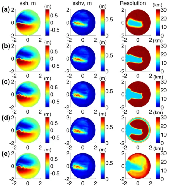
The question is to what an extent the ‘‘errors’’ of simulations on mesh C can be eliminated by using meshes CF with variable resolution. Figures 2 and 3 present, respectively, the results of simulations on these meshes and the differences between the reference case and these simulations (F-CF). In both figures the third col- umn shows the resolution of the meshes used. The coarsest and finest resolutions on these meshes are set tohc530 km andhf510 km, respectively. The resolution is a function of space specified ashðx;yÞ5hc=r, whereris the refinement factor, which is between 1 and 3 (hc=hf).
When constructing the variable-resolution meshes we applied two approaches. In the first one (for meshes CF1–CF4), the std of SSH ‘‘observed’’ on mesh F was smoothed with a square box filter of 100 km in size and the area where the value exceeds the threshold ofst50:17 m was selected to be refined. This cutoff value is slightly higher than the std of SSH in the bulk of subtropical and subpolar gyres, but already much lower than the high variability along the main jet. The mesh refinement factor r is set to 3 inside the high- variability domain identified by the threshold and to 1 elsewhere, with the sharp boundary between the coarse and fine domains smoothed with a box filter (200 km in size). Mesh CF1 follows this approach
exactly, and meshes CF2–4 were obtained by augmenting CF1 by adding extra refined regions. In the sec- ond approach, followed by mesh CF5, the resolution was determined by a low-pass filtered pattern of SSHV as explained in the Appendix.
The mean SSH and SSHV simulated on mesh CF1 are shown in the first row of Figures 2 and 3. Compared to experiment C, the amplitude of the variability becomes stronger and closer to that of the reference run F.
However, the results still show noticeable deviations from the reference run. Since the refinement relies only on the ‘‘observed’’ variability, which is relatively low in the near vicinity of the jet separation point, the resolution of mesh CF1 stays coarse there. In turn, this leads to the increased dissipation and reduced ampli- tude of velocity and relative vorticity, which then results in a nearly zonal jet shed off into the ocean.
Despite the mesh refinement, the simulated mean SSH pattern in this case is more like that on the coarse mesh (see Figure 1). This indicates that the observed eddy variability alone is insufficient for designing the mesh resolution, and that one needs to take into account the existing knowledge on the flow dynamics.
On mesh CF2 we add a patch of fine resolution around the jet separation site. This substantially improves the simulated dynamics, and both the mean and variability of the SSH become closer to those in the refer- ence run (Figure 3). If we extend the added patch along the western coast (mesh CF3), the agreement improves even further. Although the improvement obtained on mesh CF3 against mesh CF2 is less
Figure 2.Mean SSH (left column) and std of SSH (middle column) on the variable resolution meshes CF1–CF5 (from top to bottom). The right column shows the mesh resolution. The axes are in 103km.
substantial than on the step from mesh CF1 to CF2, it is still visible in the difference plots shown in Figure 3.
The simulated variability depends on the presence of seed perturbations in the flow upstream the separa- tion point on both the subpolar and subtropical sides. By refining along the western coast we reduce damp- ing there, which contributes to the development of the jet instabilities. Although some difference in the mean and variability between F and CF2(3) still persist in the refined area, the improvement achieved through local mesh refinement is remarkable. It is difficult to propose a universal criterion on how to select the optimal size of the patch around the jet separation. High magnitude of relative vorticity may provide additional hints, as well as the magnitude of surface temperature gradient. However, some tuning will still be needed (cf. CF2 and CF3).
However, systematic differences from experiment F persist on meshes CF1–3 outside the refined area in the northeastern part of the subpolar gyre. By comparing these differences to the differences shown in Figure 1, we see that outside the refined region the SSHV on meshes CF1–CF3 just remains close to that on mech C. It is plausible to assume that refinement along the basin boundary could help to improve the result by reducing viscous dissipation there. In order to test this assumption, we added a band of increased resolution along the continental break on mesh CF4. As shown in Figure 3, this effort does not improve the result.
Figure 3.Same as in Figure 2 but for the differences between the reference run and simulations on respective meshes (the fields are inter- polated to a regular 10 km mesh). Patterns in the middle column are smoothed with a box filter 200 km in size to eliminate small scales associated with low (once per 10 days) sampling rate. The axes are in 103km.
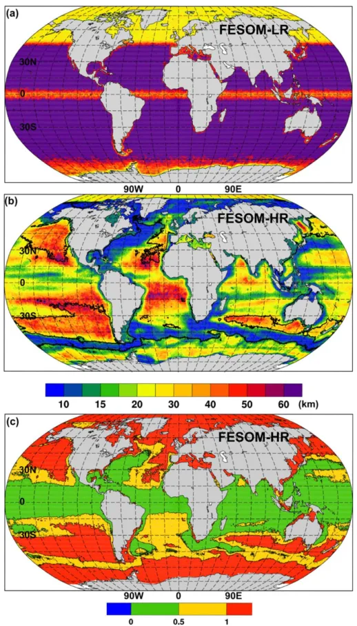
Figure 4.(a) The resolutionhof the FESOM-LR mesh. (b) The resolutionhof the FESOM-HR mesh. The contour line is the boundary where hcoincides with the internal Rossby radiusLR. (c) The ratioh=LRobtained for the FESOM-HR mesh. Green color marks eddy-resolving areas.
The Rossby radius has been estimated in the WKB approximation asLR5ð1=pfÞÐ0
2HNdz, whereNis the Brunt–V€ais€al€a frequency.
In contrast, clear improvement is obtained on mesh CF5, which is refined using a function of the SSHV simulated on mesh F.
The finest resolutionhfwas set to 10 km, the coarsest,hc, to 30 km and the thresh- old variability levelstto 0.5 m (see Appen- dix for the procedure). Additionally, the resolution along the western coast is also refined as on mesh CF3.
Compared to mesh CF3, the method used here leads to a slightly reduced resolution over the area with high variability but increases it over the eastern part of subpolar gyre, as is seen in Figure 3. The total num- ber of grid nodes on mesh CF5 remains close to that on mesh CF3. Simulations on mesh CF5 show a reduced bias in the northern and eastern parts of the subpolar gyre observed on meshes CF1–3, yet agree the same well in the area around the jet characterized by the highest variability.
2.3. Remarks
Among the variable resolution meshes, CF5 showed the best skill. This mesh has 47 thousand surface grid nodes, about one third of the reference mesh (133 thousand). As the model time step is determined by the finest resolution (10 km), the same on both meshes, CF5 helps to reduce the computational cost by a factor of three. In this idealized model configuration, the model domain is rather small and the area with high SSHV occupies a relatively large portion of the total domain. In the real ocean, the ratio between areas with high and low SSHV is smaller than in this idealized setup, implying potentially greater saving in computa- tional cost with variable meshes. Since most of the computational nodes (about 80%) are located in the fine resolution area, using the time stepping dictated by the fine mesh in our applications does not induce sig- nificant loss in model efficiency. The approach to design meshes used for CF5 proves to be more flexible than its simpler counterpart used for CF1–4. Yet in the end they both are sensitive to the selected threshold variability value which can be lower for the former if the meshes should be of same computational cost.
The above comparison also stresses that the knowledge of variability alone is insufficient for designing mesh resolution, and additional information on the ocean dynamics has to be used.
3. Global Ocean Simulations
Compared to the idealized experiment, simulations of the global ocean circulation present more challenges.
First, there are many regions with high variability and resolving all them may be prohibitive; many dynami- cally important regions in the ocean do not have very high SSHV yet need high resolution; and the resolu- tion needed to adequately simulate the observed dynamics is generally not well known. Second, the
Table 1.LR and HR Setups
Surface Nodes Time Step Run Time CPUs
LR 127.000 30 min 20 yr/d 240
HR 1.300.000 10 min 6 yr/d 2400
Figure 5.A snapshot of the ocean speed at 50 m from FESOM-HR in the logarithmic scale (log10juj=u0withuthe simulated velocity in m/s andu051 m/s).
Rossby radius of deformation varies strongly over the ocean, and so does the resolution needed to repre- sent eddies. The approaches applied above have to be modified to take this variation into account. Third, one needs to tune eddy parameterizations especially in areas with transitional resolution. Finally, the met- rics of model performance commonly include the behavior of watermasses and circulation, not solely the simulated variability. Exploring all these aspects is beyond the scope of this work. The goal of this section is rather to illustrate what can be achieved on the global ocean scale with the SSHV-based mesh design method.
3.1. Model Setups
We compare simulations carried out with two global ocean setups of FESOM. The first one employs a coarse mesh with nominal resolution of about 18in the global ocean, about 25 km north of 50N, about 1/38in the equatorial band, and moderate refinement along the coasts. This setup was used in the CORE-II inter- comparison project (seeDanabasoglu[2014] and other CORE-II papers). Its performance is similar to other ocean models with close resolution. This setup is further referred to as FESOM-LR (low resolution). It has about 1.27105surface grid nodes (see Figure 4a).
The second setup uses a locally eddy-resolving mesh. Its design follows the approach of mesh CF5 and relies on the AVISO satellite altimetry product [Le Traon et al., 1998;Ducet et al., 2000]. The coarsest resolu- tion on this mesh is set to 60 km, and the finest resolution is 10 km. The refinement was determined by a low-pass filtered SSHV pattern (see the Appendix) derived from the AVISO data. Fine resolution is obtained
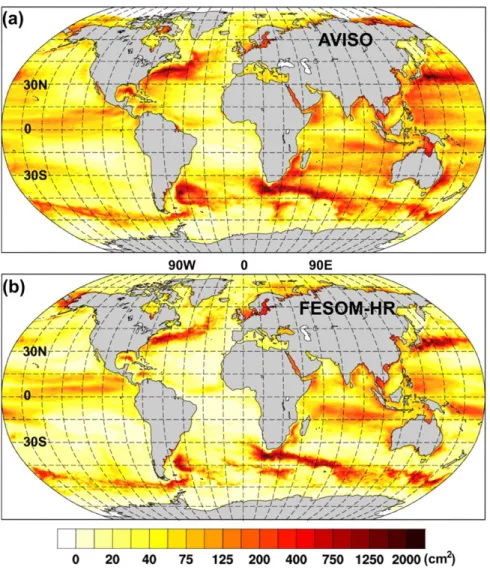
Figure 6.The SSHV (cm2) in (a) observations (AVISO) and (b) simulated by FESOM-HR.
in regions with high SSHV, including the passways of main currents — the Gulf Stream, Kuroshio, Antarctic Cir- cumpolar Current (ACC) and Agulhas Current (see Figure 4b for the mesh resolution). In addition to the mesh refinement based on SSHV, the resolution is also refined along the western coast upstream the separation loca- tions of Gulf Stream and Kuroshio, as suggested by the finding in section 2. Further refinements are in the Nordic Seas and margional seas in the Arctic Ocean. This setup is referred to as FESOM-HR (high resolution).
The mesh contains about 1.3106surface grid nodes, which is close to the number of nodes on a Mercator 1/
48mesh (only wet nodes are dealt with on unstructured meshes). This mesh size was also selected to ensure reasonably fast simulations with available computational resources. The LR and HR global setups are run with time steps of 30 and 10 min respectively, which allows for about 20 (on LR) and 6 (on HR) simulation years per day. Note that the computational resources used for LR and HR setups are different. Whereas the LR setup was run on 240 CPUs, HR setup used 2400. The summary of both setups is presented in Table 1.
The contour lines in the middle panel of Figure 4 show the boundaries where the mesh resolution coincides with the internal Rossby radiusLR, and the bottom panel displays the ratio ofh=LR. Due to the selected refinement resolution and the constraint on the total number of grid nodes, the areas where the mesh is eddy-resolving (h<LR=2) are of limited size. Outside the615belt around the equator, the mesh is eddy resolving only around the Gulf Stream, Kuroshio, BrazilMalvinas Confluence Zone and the Agulhas region.
The largest part of refined area in the Southern Ocean stays eddy permitting, and the same for the North Atlantic Current. Both setups have the same 47z-coordinate vertical levels. They are spun up for 30 years, then run for 60 years from 1948 to 2007 driven by the CORE-II forcing [Large and Yeager, 2009].
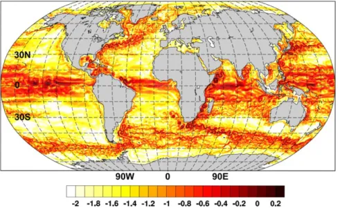
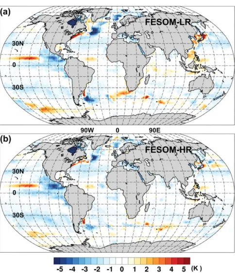
Figure 7.The bias in temperature averaged over the upper 100 m with respect to the GDEM climatology for (a) FESOM-LR and (b) FESOM- HR.
3.2. Results
Figure 5 presents a snapshot of the near-surface velocity (50 m) obtained on the HR mesh. It qualitatively shows that refining the mesh following the observed SSHV leads to the expected pattern of main ocean currents with eddies. Strong eddying flow is simulated over the eddy permitting and eddy-resolving parts of the mesh (Figure 4).
The SSHV simulated by the HR setup is validated against the AVISO product in Figure 6. Note that we do not show the variability of the LR run because its coarse mesh generally cannot produce high SSHV as expected.
The SSHV is calculated based on 5 day means, and we found that using daily means gives very similar results.
There is a good agreement with the altimetry product in terms of the spatial pattern of SSHV in the refined regions, including ACC, Kuroshio, Gulf Stream and the Agulhas Current, but not in the areas where the resolu- tion was left intentionally coarse. This indicates that the approach applied to the mesh design performs well.
However, because mesh HR is eddy resolving only over limited patches, the simulated variability remains lower than in the observations. Note, that the atmospheric pressure loading is not taken into account in the model, which may also contribute to simulate lower SSHV than the observation. The performance in representing the SSHV varies among the refined regions. For example, in the Southern Ocean the high-resolution areas are nar- row and not eddy-resolving, and transitions to coarse mesh are sharp, yet the overall performance is not less satisfactory than in the Gulf Stream region, where the refined mesh occupies a wider area. Clearly, in order to improve the agreement one needs to widen the eddy-permitting patches and, perhaps, to further increase resolution over some of these regions, which is the subject of future work.
While the simulated SSHV is a direct indicator of the success of the concept, in the case of realistic ocean one is more interested in the simulated ocean state. Its detailed assessment is beyond the scope of this work, and we present here only examples showing the improvements brought about by the increased resolution. Figure 7 compares the model bias in temperature averaged over the upper 100 m, referenced to the GDEM climatology [Carnes, 2009]. The results are averaged over the last 10 years. The top panel shows the LR case, which has biases common to models of comparable resolution in regions with high SSHV (the north-west corner, Agulhas Current, Southern Ocean). The biases are generally reduced on mesh HR (bottom panel). The bias in the eastern equatorial Pacific is, however, not visibly different on the two meshes and is localized in the upper ocean. Pre- sumably it reflects some transient variability which is not fully eliminated by averaging. Another possible expla- nation might be a persistent bias due to common forcing anomalies or omitted physical processes.
High resolution helps to reduce model biases through explicit representation of dynamical processes medi- ated by eddies. Judged by the surface temperature bias, resolving eddies seems to outperform the eddy parameterization in the FESOM simulations used in this work. Globally calculated RMS error for the vertically averaged 0–100 m temperature is 0.97K for HR and 1.07K for the LR setup. It shall be mentioned, that in the deeper ocean layers (from 200 to 700 m) the results do not change significantly. The spatial pattern of the bias is similar and its strength is reduced in HR setup. The refined resolution does not only imply the pres- ence of eddies, but also lower dissipation. The improved representation of the pathway of the North
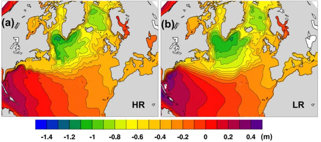
Figure 8.Mean SSH for (a) FESOM-HR and (b) FESOM-LR.
Atlantic Current on mesh HR is seemingly related to this. On mesh HR the current follows a more northern pathway than on LR, which reduces the cold bias in the northwest corner. This can be illustrated by the dif- ference in mean SSH between HR and LR (Figure 8). The SSH increases by about 0.4 m in the north west cor- ner as a consequence of the shift of the path of the North Atlantic Current and modification of the Subpolar Gyre.
4. Discussion and Conclusion
The examples considered above show that the mesh refinement based on the observed variability improves the agreement of simulated variability with observations. However, the information on SSHV alone is insuffi- cient. Better agreement can be obtained if the refinement also takes into account the existing knowledge of the ocean dynamics, for example, to include the areas upstream the mid latitude jets. The proposed approach to design variable-resolution meshes needs to be augmented to fully use the advantage of unstructured meshes. Most importantly, the scaling of resolution with the internal Rossby radius has to be introduced, which is absent in the examples above. The mesh design strategy may also depend on practical limitations. If the mesh size is chosen to be about the size of a uniform 1/48mesh, as in the example above, the eddy-resolving part of the global mesh can only cover limited areas and the overall model performance stays on the level of an eddy-permitting model. This implies that meshes of larger size (about 2–33106sur- face nodes) have to be used to be eddy-resolving in most of the dynamically key regions.
The real ocean simulations presented in this work show that the variable-resolution mesh helps to reduce the model bias in hydrography. More studies are needed to quantify the effects of locally resolved eddy dynamics. The results also imply that resolving eddies in high-resolution models can produce better mean flow pathways and water mass properties than using eddy parameterizations in low-resoltion models. Gen- erally, improving resolution-dependent parameterization schemes is needed for unstructured-mesh models.
Our simulation is done in a forced ocean run. It remains to see whether the improved ocean circulation and hydrography can help to reduce model uncertainty in coupled climate models.
The observed SSHV is an obvious indicator of places where eddy variability is strong, but the choice of resolu- tion can also be based on the analysis of isopycnal slopes or the Eady growth rate. We did not explore these possibilities here. They can be helpful over the regions where reliable measurements of SSHV are not available.
We would like to repeat that numerical efficiency of setups presented here depends on their time step which is largely set by the smallest mesh elements (10 km for both the idealized case and the global mesh HR). The implication is that the area occupied by the fine mesh should contain a dominant part of grid nodes (as on mesh HR), otherwise using the same time step size for both high and low resolution areas would mean an effective reduction in model efficiency. Because of good parallel scalability of the models used in this study, the simulation throughput is determined mainly by time step size (provided the availabil- ity of super-computer cores). The LR and HR global setups are run with time steps of 30 and 10 min respec- tively, which allows for about 20 (on LR) and 6 (on HR) simulation years per day.
To conclude, in this work we proposed and examined an approach for selecting resolution in models formu- lated on unstructured meshes which can be useful for large-scale ocean simulations. It uses the standard deviation of the observed sea surface height as a main criterion for mesh refinement. It has to be adjusted in practice based on other existing knowledge of ocean dynamics. We demonstrated that the mesh refine- ment using this approach can improve the representation of both eddy variability and ocean hydrography.
The real ocean simulations shown here serve to illustrate the approach and stimulate discussions on unstructured-mesh model development.
Appendix
Assume that the SSHVsis known on a regular mesh. We use the variability interpolated to a 10 km mesh for the gyre test case and the altimetry product on a global 0.258mesh for the FESOM case. The procedure consist of several steps.
1. Define the threshold variability levelst(as some fraction of maximum SSHV),hc,hfandrmax5hc=hf. 2. Set the initial refinement distributionr05maxð1;minðs=st;rmaxÞÞ.
3. Adjust the pattern ofr0by settingr05rmaxin the areas where the refinement has to be made independ- ent of the ratios=standr051 in areas that should stay coarse. Various additional factors can be taken into account on this stage.
4. Iteraterk115rk1R2Drk;k50;1;. . .N, andr5rN, whereDis the Laplacian operator,N is the number of iterations, andRN1=2sets the distance of diffusive spreading. The distanceRis a function of horizontal location for the FESOM case, with larger values over the Gulf Stream area to provide some extra spread- ing. To warrant numerical stability of iterationsRis a fraction of the regular mesh resolution, and the desired spreading is controlled by the number of iterationsN.
All steps of this procedure require experimenting, and all they may be extended further. The threshold vari- ability has the sense of error tolerance, but also defines the size of refined areas. The total number of nodes can only be estimated whenris computed, so the procedure is repeated with adjusted values ofst,hfand hcto fit the mesh size bound.
A similar in spirit filtering can be done by solving the equation2R2Dr1r5r0for the mesh refinement factor r. Here,Rhas the sense of the correlation radius. It, however, requires an iterative solver for large meshes and is therefore less convenient.
References
Carnes, M. R. (2009),Description and Evaluation of GDEM-V 3.0, Naval Res. Lab., Stennis Space Cent., Hancock, Miss.
Danabasoglu, G. (2014), North Atlantic simulations in Coordinated Ocean-ice Reference Experiments phase II (CORE-II). Part I: Mean states, OceanModell.,73, 76–107.
Danilov, S. (2012), Two finite-volume unstructured mesh models for large-scale ocean modeling,Ocean Modell.,47, 1425, doi:10.1016/
j.ocemod.2012.01.004.
Danilov, S., and A. Androsov (2015), Cell-vertex discretization of shallow water equations on mixed unstructured meshes,Ocean Dyn.,65, 33–47, doi:10.1007/s10236-014-0790-x.
Danilov, S., and Q. Wang (2015), Resolving eddies by local mesh refinement,Ocean Modell.,93, 7583.
Ducet, N., P.-Y. Le Traon, and G. Reverdin (2000), Global high-resolution mapping of ocean circulation from TOPEX/Poseidon and ERS-1 and22,J. Geophys. Res.,105, 19,477–19,498.
Durgadoo, J. V., B. R. Loveday, C. J. C. Reason, P. Penven, and A. Biastoch (2013), Agulhas leakage predominantly responds to the Southern Hemisphere westerlies,J. Phys. Oceanogr.,43, 2113–2131.
Fox-Kemper, B., and D. Menemenlis (2008), Can large eddy simulation techniques improve mesoscale rich ocean models?, in1679 Ocean Modeling in an Eddying Regime, Geophys. Monogr. 177, edited by M. W. Hecht and H. Hasumi, 409 pp., AGU, Washington, D. C.
Griffies, S., et al. (2015), Impacts on ocean heat from transient mesoscale eddies in a hierarchy of climate models,J. Clim.,28, 952–977, doi:10.1175/JCLI-D-14-00353.1.
Hallberg, R. (2013), Using a resolution function to regulate parameterizations of oceanic mesoscale eddy effects.Ocean Modell.,72, 92–103.
Kawasaki, T., and H. Hasumi (2014), Effect of freshwater from the West Greenland Current on the winter deep convection in the Labrador Sea,Ocean Modell.,75, 51–64.
Large, W. G., and S. G. Yeager (2009), The global climatology of an interannually varying air-sea flux data set,Clim. Dyn.,33, 341–364.
Le Traon, P.-Y., F. Nadal, and N. Ducet (1998), An improved mapping method of multi-satellite altimeter data,J. Atmos. Oceanic Technol.,15, 522–534.
Ringler, T., M. Petersen, R. Higdon, D. Jacobsen, M. Maltrud, and P. W. Jones (2013), A multi-resolution approach to global ocean modelling, Ocean Modell.,69, 211–232.
Sein, D. V., U. Mikolajewicz, M. Gr€oger, I. Fast, W. Cabos, J. G. Pinto, S. Hagemann, T. Semmler, A. Izquierdo, and D. Jacob (2015), Regionally coupled atmosphere-ocean-sea ice-marine biogeochemistry model ROM: 1. Description and validation,J. Adv. Model. Earth Syst.,7, 268–304, doi:10.1002/2014MS000357.
Sidorenko, D., et al. (2015), Towards multi-resolution global climate modeling with ECHAM6FESOM. Part I: Model formulation and mean cli- mate,Clim. Dyn.,44(3–4), 757–780.
Small, J., E. Curchitser, K. Hedstrom, B. Kauffman, and W. Large (2015), The Benguella upwelling system: Quantifying the sensitivity to reso- lution and coastal representation in a global climate model,J. Clim.,28, 9409–9432, doi:10.1175/JCLI-D-15-0192.1.
Talandier, C., J. Deshayes, A.-M. Treguier, X. Capet, R. Benshila, L. Debreu, R. Dussin, J.-M. Molines, and G. Madec 2014), Improvements of simulated Western North Atlantic current system and impacts on the AMOC,Ocean Modell.,76, 1–19.
Wang, Q., S. Danilov, D. Sidorenko, R. Timmermann, C. Wekerle, X. Wang, T. Jung, and J. Schr€oter (2014), The Finite Element Sea Ice-Ocean Model (FESOM) v.1.4: Formulation of an ocean general circulation model,Geosci. Model Dev.,7(2), 663–693, doi:10.5194/gmd-7-663- 2014.
Acknowledgments
The altimeter products were produced by Ssalto/Duacs and distributed by Aviso, with support from Cnes (http://
www.aviso.altimetry.fr/duacs/). Dmitry Sein and Jonathan Durgadoo have been supported by the German Federal Ministry of Education and Research (BMBF) under the research grant 03G0835B of the project SPACES-AGULHAS. Additionally, Dmitry Sein was supported by EC project PRIMAVERA under the grant agreement no. 641727. D. Sidorenko and Q. Wang are funded by the Helmholtz Climate Initiative REKLIM (Regional Climate Change) project. We thank both referees for the
constructive suggestions, which helped to improve the manuscript.