Quantum Mechanics

(1)

2 ^nd term 2002 Martin Plenio Imperial College

Version January 28, 2002 Office hours: Tuesdays 11am-12noon and 5pm-6pm!

Office: Blackett 622

Available at:

(2)

Part I

Quantum Mechanics

5

(7)

(8)

Introduction

This lecture will introduce quantum mechanics from a more abstract point of view than the first quantum mechanics course that you took your second year.

What I would like to achieve with this course is for you to gain a deeper understanding of the structure of quantum mechanics and of some of its key points. As the structure is inevitably mathematical, I will need to talk about mathematics. I will not do this just for the sake of mathematics, but always with a the aim to understand physics. At the end of the course I would like you not only to be able to understand the basic structure of quantum mechanics, but also to be able to solve (calculate) quantum mechanical problems. In fact, I believe that the ability to calculate (finding the quantitative solution to a problem, or the correct proof of a theorem) is absolutely essential for reaching a real understanding of physics (although physical intuition is equally important). I would like to go so far as to state

If you can’t write it down, then you do not understand it!

With ’writing it down’ I mean expressing your statement mathematically or being able to calculate the solution of a scheme that you pro- posed. This does not sound like a very profound truth but you would be surprised to see how many people actually believe that it is completely sufficient just to be able to talk about physics and that calculations are a menial task that only mediocre physicists undertake. Well, I can as- sure you that even the greatest physicists don’t just sit down and await inspiration. Ideas only come after many wrong tries and whether a try is right or wrong can only be found out by checking it, i.e. by doing some sorts of calculation or a proof. The ability to do calculations is not something that one has or hasn’t, but (except for some exceptional cases) has to be acquired by practice. This is one of the reasons why these lectures will be accompanied by problem sheets (Rapid Feedback System) and I really recommend to you that you try to solve them. It is quite clear that solving the problem sheets is one of the best ways to prepare for the exam. Sometimes I will add some extra problems to the problem sheets which are more tricky than usual. They usually intend

(9)

to illuminate an advanced or tricky point for which I had no time in the lectures.

The first part of these lectures will not be too unusual. The first chapter will be devoted to the mathematical description of the quantum mechanical state space, the Hilbert space, and of the description of physical observables. The measurement process will be investigated in the next chapter, and some of its implications will be discussed. In this chapter you will also learn the essential tools for studying entanglement, the stuff such weird things as quantum teleportation, quantum cryptography and quantum computation are made of. The third chapter will present the dynamics of quantum mechanical systems and highlight the importance of the concept of symmetry in physics and particularly in quantum mechanics. It will be shown how the momentum and angular momentum operators can be obtained as generators of the symmetry groups of translation and rotation. I will also introduce a different kind of symmetries which are called gauge symmetries. They allow us to ’derive’ the existence of classical electrodynamics from a simple invariance principle. This idea has been pushed much further in the 1960’s when people applied it to the theories of elementary particles, and were quite successful with it. In fact, t’Hooft and Veltman got a Nobel prize for it in 1999 work in this area. Time dependent problems, even more than time-independent problems, are difficult to solve exactly and therefore perturbation theoretical methods are of great importance. They will be explained in chapter 5 and examples will be given.

Most of the ideas that you are going to learn in the first five chapters of these lectures are known since about 1930, which is quite some time ago. The second part of these lectures, however, I will devote to topics which are currently the object of intense research (they are also my main area of research). In this last chapter I will discuss topics such as entanglement, Bell inequalities, quantum state teleportation, quantum computation and quantum cryptography. How much of these I can cover depends on the amount of time that is left, but I will certainly talk about some of them. While most physicists (hopefully) know the basics of quantum mechanics (the first five chapters of these lectures), many of them will not be familiar with the content of the other chapters. So, after these lectures you can be sure to know about something that quite a few professors do not know themselves! I hope that this motivates

(10)

you to stay with me until the end of the lectures.

Before I begin, I would like to thank, Vincenzo Vitelli, John Pa- padimitrou and William Irvine who took this course previously and spotted errors and suggested improvements in the lecture notes and the course. These errors are fixed now, but I expect that there are more. If you find errors, please let me know (ideally via email so that the corrections do not get lost again) so I can get rid of them.

Last but not least, I would like to encourage you both, to ask questions during the lectures and to make use of my office hours. Questions are essential in the learning process, so they are good for you, but I also learn what you have not understood so well and help me to improve my lectures. Finally, it is more fun to lecture when there is some feedback from the audience.

(11)

(12)

Chapter 1 Mathematical Foundations

Before I begin to introduce some basics of complex vector spaces and discuss the mathematical foundations of quantum mechanics, I would like to present a simple (seemingly classical) experiment from which we can derive quite a few quantum rules.

1.1 The quantum mechanical state space

When we talk about physics, we attempt to find a mathematical description of the world. Of course, such a description cannot be justified from mathematical consistency alone, but has to agree with experimental evidence. The mathematical concepts that are introduced are usually motivated from our experience of nature. Concepts such as position and momentum or the state of a system are usually taken for granted in classical physics. However, many of these have to be subjected to a careful re-examination when we try to carry them over to quantum physics. One of the basic notions for the description of a physical system is that of its ’state’. The ’state’ of a physical system essentially can then be defined, roughly, as the description of all the known (in fact one should say knowable) properties of that system and it therefore represents your knowledge about this system. The set of all states forms what we usually call the state space. In classical mechanics for example this is the phase space (the variables are then position and momentum), which is a real vector space. For a classical point-particle moving in

11

(13)

one dimension, this space is two dimensional, one dimension for position, one dimension for momentum. We expect, in fact you probably know this from your second year lecture, that the quantum mechanical state space differs from that of classical mechanics. One reason for this can be found in the ability of quantum systems to exist in coherent superpositions of states with complex amplitudes, other differences re- late to the description of multi-particle systems. This suggests, that a good choice for the quantum mechanical state space may be a complex vector space.

Before I begin to investigate the mathematical foundations of quantum mechanics, I would like to present a simple example (including some live experiments) which motivates the choice of complex vector spaces as state spaces a bit more. Together with the hypothesis of the existence of photons it will allow us also to ’derive’, or better, to make an educated guess for the projection postulate and the rules for the computation of measurement outcomes. It will also remind you of some of the features of quantum mechanics which you have already encountered in your second year course.

1.2 The quantum mechanical state space

In the next subsection I will briefly motivate that the quantum mechanical state space should be a complex vector space and also motivate some of the other postulates of quantum mechanics

1.2.1 From Polarized Light to Quantum Theory

Let us consider plane waves of light propagating along the z-axis. This light is described by the electric field vector E~ orthogonal on the direction of propagation. The electric field vector determines the state of light because in the cgs-system (which I use for convenience in this example so that I have as few₀ andµ₀ as possible.) the magnetic field is given byB~ =~e_z×E. Given the electric and magnetic field, Maxwells~ equations determine the further time evolution of these fields. In the absence of charges, we know that E(~~ r, t) cannot have a z-component,

(14)

so that we can write

E(~~ r, t) =E_x(~r, t)~e_x+E_y(~r, t)~e_y = E_x(~r, t) Ey(~r, t)

!

. (1.1)

The electric field is real valued quantity and the general solution of the free wave equation is given by

Ex(~r, t) = E_x⁰cos(kz−ωt+αx) E_y(~r, t) = E_y⁰cos(kz−ωt+α_y) .

Herek = 2π/λis the wave-number, ω= 2πν the frequency, α_x and α_y are the real phases and E_x⁰ and E_y⁰ the real valued amplitudes of the field components. The energy density of the field is given by

(~r, t) = 1

8π(E~²(~r, t) +B~²(~r, t))

= 1

4π

h(E_x⁰)²cos²(kz−ωt+α_x) + (E_y⁰)²cos²(kz−ωt+α_y)ⁱ . For a fixed position~rwe are generally only really interested in the time- averaged energy density which, when multiplied with the speed of light, determines the rate at which energy flows in z-direction. Averaging over one period of the light we obtain the averaged energy density ¯(~r) with

¯

(~r) = 1 8π

h(E_x⁰)²+ (E_y⁰)²ⁱ . (1.2) For practical purposes it is useful to introduce thecomplexfield components

E_x(~r, t) = Re(E_xeî(kz−ωt)) E_y(~r, t) =Re(E_yeî(kz−ωt)) , (1.3) with E_x =E_x⁰eîα^x and E_y =E_y⁰eîα^y. Comparing with Eq. (1.2) we find that the averaged energy density is given by

¯

(~r) = 1 8π

h|E_x|²+|E_y|²ⁱ . (1.4) Usually one works with the complex field

E(~~ r, t) = (E_x~e_x+E_y~e_y)e^i(kz−ωt)= E_x E_y

!

e^i(kz−ωt) . (1.5)

(15)

This means that we are now characterizing the state of light by a vector with complexcomponents.

The polarization of light waves are described by E_x and E_y. In the general case of complex E_x and E_y we will have elliptically polarized light. There are a number of important special cases (see Figures 1.1 for illustration).

1. E_y = 0: linear polarization along the x-axis.

2. E_x = 0: linear polarization along the y-axis.

3. E_x =E_y: linear polarization along 45⁰-axis.

4. Ey =iEx: Right circularly polarized light.

5. E_y =−iE_x: Left circularly polarized light.

Figure 1.1: Left figure: Some possible linear polarizations of light, horizontally, vertically and 45 degrees. Right figure: Left- and right- circularly polarized light. The light is assumed to propagate away from you.

In the following I would like to consider some simple experiments for which I will compute the outcomes using classical electrodynamics. Then I will go further and use the hypothesis of the existence of photons to derive a number of quantum mechanical rules from these experiments.

Experiment I:Let us first consider a plane light wave propagating in z-direction that is falling onto an x-polarizer which allows x-polarized

(16)

light to pass through (but not y polarized light). This is shown in figure 1.2. After passing the polarizer the light is x-polarized and from

Figure 1.2: Light of arbitrary polarization is hitting a x-polarizer.

the expression for the energy density Eq. (1.4) we find that the ratio between incoming intensity I_in (energy density times speed of light) and outgoing intensity I_out is given by

I_out

I_in = |E_x|²

|E_x|²+|E_y|². (1.6) So far this looks like an experiment in classical electrodynamics or optics.

Quantum Interpretation: Let us change the way of looking at this problem and thereby turn it into a quantum mechanical experiment. You have heard at various points in your physics course that light comes in little quanta known as photons. The first time this assumption had been made was by Planck in 1900 ’as an act of desperation’ to be able to derive the blackbody radiation spectrum. Indeed, you can also observe in direct experiments that the photon hypothesis makes sense.

When you reduce the intensity of light that falls onto a photodetector, you will observe that the detector responds with individual clicks each triggered by the impact of a single photon (if the detector is sensitive enough). The photo-electric effect and various other experiments also confirm the existence of photons. So, in the low-intensity limit we have to consider light as consisting of indivisible units called photons. It is a fundamental property of photons that they cannot be split – there is no such thing as half a photon going through a polarizer for example.

In this photon picture we have to conclude that sometimes a photon will be absorbed in the polarizer and sometimes it passes through. If the photon passes the polarizer, we have gained one piece of information, namely that the photon was able to pass the polarizer and that therefore it has to be polarized in x-direction. The probability p for

(17)

the photon to pass through the polarizer is obviously the ratio between transmitted and incoming intensities, which is given by

p= |E_x|²

|E_x|²+|E_y|² . (1.7) If we write the state of the light with normalized intensity

E~_N = E_x

q|E_x|²+|E_y|²~e_x+ E_y

q|E_x|²+|E_y|²~e_y , (1.8) then in fact we find that the probability for the photon to pass the x- polarizer is just the square of the amplitude in front of the basis vector

~e_x! This is just one of the quantum mechanical rules that you have learned in your second year course.

Furthermore we see that the state of the photon after it has passed the x-polarizer is given by

E~_N =~e_x , (1.9)

ie the state has has changed from ^E_E^x

y

to ^E₀^x. This transformation of the state can be described by a matrix acting on vectors, ie

E_x 0

= 1 0

0 0

! E_x E_y

!

(1.10) The matrix that I have written here has eigenvalues 0 and 1 and is therefore a projection operator which you have heard about in the second year course, in fact this reminds strongly of the projection postulate in quantum mechanics.

Experiment II: Now let us make a somewhat more complicated experiment by placing a second polarizer behind the first x-polarizer.

The second polarizer allows photons polarized in x⁰ direction to pass through. If I slowly rotate the polarizer from the x direction to the y direction, we observe that the intensity of the light that passes through the polarizer decreases and vanishes when the directions of the two polarizers are orthogonal. I would like to describe this experiment mathematically. How do we compute the intensity after the polarizer

(18)

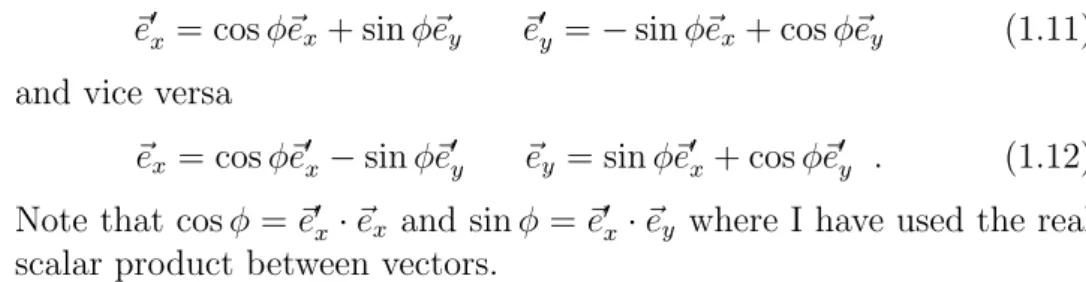
now? To this end we need to see how we can express vectors in the basis chosen by the direction x⁰ in terms of the old basis vectors~ex, ~ey. The new rotated basis~e⁰_x, ~e⁰_y (see Fig. 1.3) can be expressed by the old basis by

~e⁰_x = cosφ~e_x+ sinφ~e_y ~e⁰_y =−sinφ~e_x+ cosφ~e_y (1.11) and vice versa

~ex = cosφ~e⁰_x−sinφ~e⁰_y ~ey = sinφ~e⁰_x+ cosφ~e⁰_y . (1.12) Note that cosφ =~e⁰_x·~e_x and sinφ =~e⁰_x·~e_y where I have used the real scalar product between vectors.

Figure 1.3: The x’- basis is rotated by an angle φ with respect to the original x-basis.

The state of the x-polarized light after the first polarizer can be rewritten in the new basis of the x’-polarizer. We find

E~ =Ex~ex =Excosφ~e⁰_x−Exsinφ~e⁰_y =Ex(~e⁰_x·~ex)~e⁰_x−Ex(~e⁰_y·~ey)~e⁰_y Now we can easily compute the ratio between the intensity before and after the x⁰-polarizer. We find that it is

I_{af ter}

I_{bef ore} =|~e⁰_x·~ex|² =cos²φ (1.13) or if we describe the light in terms of states with normalized intensity as in equation 1.8, then we find that

I_{af ter} Ibef ore

=|~e⁰_x·E~_N|² = |~e⁰_x·E~_N|²

|~e⁰_x·E~_N|²+|~e⁰_y·E~_N|² (1.14)

(19)

where E~_N is the normalized intensity state of the light after the x- polarizer. This demonstrates that the scalar product between vectors plays an important role in the calculation of the intensities (and therefore the probabilities in the photon picture).

Varying the angleφ between the two bases we can see that the ratio of the incoming and outgoing intensities decreases with increasing angle between the two axes until the angle reaches 90^o degrees.

Interpretation: Viewed in the photon picture this is a rather surprising result, as we would have thought that after passing the x- polarizer the photon is ’objectively’ in the x-polarized state. However, upon probing it with anx⁰-polarizer we find that it also has a quality of anx⁰-polarized state. In the next experiment we will see an even more worrying result. For the moment we note that the state of a photon can be written in different ways and this freedom corresponds to the fact that in quantum mechanics we can write the quantum state in many different ways as a quantum superpositions of basis vectors.

Let us push this idea a bit further by using three polarizers in a row.

Experiment III:If after passing the x-polarizer, the light falls onto a y-polarizer (see Fig 1.4), then no light will go through the polarizer because the two directions are perpendicular to each other. This sim-

Figure 1.4: Light of arbitrary polarization is hitting a x-polarizer and subsequently a y-polarizer. No light goes through both polarizers.

ple experimental result changes when we place an additional polarizer between the x and the y-polarizer. Assume that we place a x’-polarizer between the two polarizers. Then we will observe light after the y- polarizer (see Fig. 1.5) depending on the orientation of x⁰. The light after the last polarizer is described by ˜E_y~e_y. The amplitude ˜E_y is calcu- lated analogously as in Experiment II. Now let us describe the (x-x’-y) experiment mathematically. The complex electric field (without the time dependence) is given by

(20)

Figure 1.5: An x’-polarizer is placed in between an x-polarizer and a y-polarizer. Now we observe light passing through the y-polarizer.

before the x-polarizer:

E~₁ =E_x~e_x+E_y~e_y. after the x-polarizer:

E~2 = (E~1~ex)~ex =Ex~ex =Excosφ~e⁰_x−Exsinφ~e⁰_y. after the x’-polarizer:

E~₃ = (E~₂~e⁰_x)~e⁰_x =E_xcosφ~e⁰_x =E_xcos²φ~e_x+E_xcosφsinφ~e_y. after the y-polarizer:

E~₄ = (E~₃~e_y)~e_y =E_xcosφsinφ~e_y = ˜E_y~e_y.

Therefore the ratio between the intensity before the x’-polarizer and after the y-polarizer is given by

I_{af ter}

I_{bef ore} = cos²φsin²φ (1.15) Interpretation: Again, if we interpret this result in the photon picture, then we arrive at the conclusion, that the probability for the photon to pass through both the x’ and the y polarizer is given by cos²φsin²φ. This experiment further highlights the fact that light of one polarization may be interpreted as a superposition of light of other polarizations. This superposition is represented by adding vectors with complex coefficients. If we consider this situation in the photon picture we have to accept that a photon of a particular polarization can also be interpreted as a superposition of different polarization states.

(21)

Conclusion: All these observations suggest that complex vectors, their amplitudes, scalar products and linear transformations between complex vectors are the basic ingredient in the mathematical structure of quantum mechanics as opposed to the real vector space of classical mechanics. Therefore the rest of this chapter will be devoted to a more detailed introduction to the structure of complex vector-spaces and their properties.

Suggestions for further reading:

G. Baym Lectures on Quantum Mechanics, W.A. Benjamin 1969.

P.A.M. Dirac, The principles of Quantum Mechanics, Oxford Univer- sity Press 1958

End of 1^stlecture

1.2.2 Complex vector spaces

I will now give you a formal definition of a complex vector space and will then present some of its properties. Before I come to this definition, I introduce a standard notation that I will use in this chapter. Given some set V we define

Notation:

1. ∀|xi ∈V means: For all |xi that lie in V.

2. ∃|xi ∈V means: There exists an element |xi that lies in V. Note that I have used a somewhat unusual notation for vectors. I have replaced the vector arrow on top of the letter by a sort of bracket around the letter. I will use this notation when I talk about complex vectors, in particular when I talk about state vectors.

Now I can state the definition of the complex vector space. It will look a bit abstract at the beginning, but you will soon get used to it, especially when you solve some problems with it.

Definition 1 Given a quadruple (V,C,+,·) where V is a set of objects (usually called vectors), C denotes the set of complex numbers,

(22)

0+⁰ denotes the group operation of addition and ⁰·⁰ denotes the multiplication of a vector with a complex number. (V,C,+,·) is called a complex vector space if the following properties are satisfied:

1. (V,+) is an Abelian group, which means that

(a) ∀|ai,|bi ∈V ⇒ |ai+|bi ∈V. (closure)

(b) ∀|ai,|bi,|ci ∈ V ⇒ |ai + (|bi +|ci) = (|ai + |bi) + |ci.

(associative)

(c) ∃|Oi ∈V so that ∀|ai ∈V ⇒ |ai+|Oi=|ai. (zero) (d) ∀|ai ∈V : ∃(−|ai)∈V so that|ai+(−|ai) =|Oi.(inverse) (e) ∀|ai,|bi ∈V ⇒ |ai+|bi=|bi+|ai. (Abelian) 2. The Scalar multiplication satisfies

(a) ∀α ∈C,|xi ∈V ⇒α|xi ∈V

(b) ∀|xi ∈V ⇒1· |xi=|xi (unit)

(c) ∀c, d∈C,|xi ∈V ⇒(c·d)· |xi=c·(d· |xi) (associative) (d) ∀c, d∈C,|xi,|yi ∈V ⇒c·(|xi+|yi) = c· |xi+c· |yi

and (c+d)· |xi=c· |xi+c· |yi. (distributive) This definition looks quite abstract but a few examples will make it clearer.

Example:

1. A simple proof

I would like to show how to prove the statement 0· |xi = |Oi.

This might look trivial, but nevertheless we need to prove it, as it has not been stated as an axiom. From the axioms given in Def.

1 we conclude.

|Oi ^(1d)₌ −|xi+|xi

(2b)

= −|xi+ 1· |xi

= −|xi+ (1 + 0)· |xi

(2d)

= −|xi+ 1· |xi+ 0· |xi

(23)

(2b)

= −|xi+|xi+ 0· |xi

(1d)

= |Oi+ 0· |xi

(1c)

= 0· |xi . 2. The C²

This is the set of two-component vectors of the form

|ai= a₁ a2

!

, (1.16)

where thea_i are complex numbers. The addition and scalar multiplication are defined as

a1

a₂

!

+ b1

b₂

!

:= a1 +b1

a₂ +b₂

!

(1.17)

c· a₁ a₂

!

:= c·a₁ c·a₂

!

(1.18) It is now easy to check that V = C² together with the addition and scalar multiplication defined above satisfy the definition of a complex vector space. (You should check this yourself to get some practise with the axioms of vector space.) The vector space C² is the one that is used for the description of spin-¹₂ particles such as electrons.

3. The set of real functions of one variable f :R→R The group operations are defined as

(f₁+f₂)(x) := f₁(x) +f₂(x) (c·f)(x) := c·f(x)

Again it is easy to check that all the properties of a complex vector space are satisfied.

4. Complex n×n matrices

The elements of the vector space are M =







m₁₁ . . . m_1n ... . .. ... mn1 . . . mnn







, (1.19)

(24)

where the m_ij are arbitrary complex numbers. The addition and scalar multiplication are defined as







a₁₁ . . . a_1n ... . .. ... a_n1 . . . a_nn





+







b₁₁ . . . b_1n ... . .. ... b_n1 . . . b_nn





 =







a₁₁+b₁₁ . . . a_1n+b_1n ... . .. ... a_n1+b_n1 . . . a_nn+b_nn





 ,

c·







a₁₁ . . . a_1n ... . .. ... a_n1 . . . a_nn







=







c·a₁₁ . . . c·a_1n ... . .. ... c·a_n1 . . . c·a_nn







.

Again it is easy to confirm that the set of complexn×n matrices with the rules that we have defined here forms a vector space.

Note that we are used to consider matrices as objects acting on vectors, but as we can see here we can also consider them as elements (vectors) of a vector space themselves.

Why did I make such an abstract definition of a vector space? Well, it may seem a bit tedious, but it has a real advantage. Once we have introduced the abstract notion of complex vector space anything we can prove directly from these abstract laws in Definition 1 will hold true for any vector space irrespective of how complicated it will look superficially. What we have done, is to isolate the basic structure of vector spaces without referring to any particular representation of the elements of the vector space. This is very useful, because we do not need to go along every time and prove the same property again when we investigate some new objects. What we only need to do is to prove that our new objects have an addition and a scalar multiplication that satisfy the conditions stated in Definition 1.

In the following subsections we will continue our exploration of the idea of complex vector spaces and we will learn a few useful properties that will be helpful for the future.

1.2.3 Basis and Dimension

Some of the most basic concepts of vector spaces are those of linear independence, dimension and basis. They will help us to express vec-

(25)

tors in terms of other vectors and are useful when we want to define operators on vector spaces which will describe observable quantities.

Quite obviously some vectors can be expressed by linear combinations of others. For example

1 2

!

= 1

0

!

+ 2· 0 1

!

. (1.20)

It is natural to consider a given set of vectors {|xi₁, . . . ,|xi_k} and to ask the question, whether a vector in this set can be expressed as a linear combination of the others. Instead of answering this question directly we will first consider a slightly different question. Given a set of vectors {|xi₁, . . . ,|xi_k}, can the null vector |Oican be expressed as a linear combination of these vectors? This means that we are looking for a linear combination of vectors of the form

λ1|xi₁+. . .+λ2|xi_k =|Oi . (1.21) Clearly Eq. (1.21) can be satisfied when all theλ_i vanish. But this case is trivial and we would like to exclude it. Now there are two possible cases left:

a) There is no combination of λ_i’s, not all of which are zero, that satisfies Eq. (1.21).

b) There are combinations of λ_i’s, not all of which are zero, that satisfy Eq. (1.21).

These two situations will get different names and are worth the Definition 2 A set of vectors {|xi₁, . . . ,|xi_k}is called linearly independent if the equation

λ₁|xi₁+. . .+λ₂|xi_k=|Oi (1.22) has only the trivial solution λ₁ =. . .=λ_k = 0.

If there is a nontrivial solution to Eq. (1.22), i.e. at least one of the λ_i 6= 0, then we call the vectors {|xi₁, . . . ,|xi_k} linearly dependent.

Now we are coming back to our original question as to whether there are vectors in {|xi₁, . . . ,|xi_k} that can be expressed by all the other vectors in that set. As a result of this definition we can see the following

(26)

Lemma 3 For a set oflinearly independentvectors{|xi₁, . . . ,|xi_k}, no |xi_i can be expressed as a linear combination of the other vectors, i.e. one cannot find λ_j that satisfy the equation

λ₁|xi₁+. . .+λi−1|xi_i−1+λ_i+1|xi_i+1+. . .+λ_k|xi_k=|xi_i . (1.23) In a set oflinearly dependentvectors{|xi₁, . . . ,|xi_k}there is at least one |xi_i that can be expressed as a linear combination of all the other

|xi_j.

Proof: Exercise! ₂

Example: The set {|Oi}consisting of the null vector only, is linearly dependent.

In a sense that will become clearer when we really talk about quantum mechanics, in a set of linearly independent set of vectors, each vector has some quality that none of the other vectors have.

After we have introduced the notion of linear dependence, we can now proceed to define the dimension of a vector space. I am sure that you have a clear intuitive picture of the notion of dimension. Evidently a plain surface is 2-dimensional and space is 3-dimensional. Why do we say this? Consider a plane, for example. Clearly, every vector in the plane can be expressed as a linear combination of any two linearly independent vectors|ei₁,|ei₂. As a result you will not be able to find a set of three linearly independent vectors in a plane, while two linearly independent vectors can be found. This is the reason to call a plane a two-dimensional space. Let’s formalize this observation in

Definition 4 Thedimensionof a vector spaceV is the largest number of linearly independent vectors in V that one can find.

Now we introduce the notion of basisof vector spaces.

Definition 5 A set of vectors {|xi₁, . . . ,|xi_k} is called a basis of a vector space V if

(27)

a) |xi₁, . . . ,|xi_k are linearly independent.

b) ∀|xi ∈V :∃λi ∈C⇒x=^P^k_i=1λi|xi_i.

Condition b) states that it is possible to write every vector as a linear combination of the basis vectors. The first condition makes sure that the set{|xi₁, . . . ,|xi_k}is the smallest possible set to allow for condition b) to be satisfied. It turns out that any basis of anN-dimensional vector space V contains exactly N vectors. Let us illustrate the notion of basis.

Example:

1. Consider the space of vectorsC² with two components. Then the two vectors

|xi₁ = 1 0

!

|xi₂ = 0 1

!

. (1.24)

form a basis ofC². A basis for the C^N can easily be constructed in the same way.

2. An example for an infinite dimensional vector space is the space of complex polynomials, i.e. the set

V ={c₀+c₁z+. . .+c_kz^k|arbitrary k and ∀c_i ∈C} . (1.25) Two polynomials are equal when they give the same values for all z ∈C. Addition and scalar multiplication are defined coefficient wise. It is easy to see that the set {1, z, z², . . .} is linearly independent and that it contains infinitely many elements. Together with other examples you will prove (in the problem sheets) that Eq. (1.25) indeed describes a vector space.

End of 2^ndlecture

1.2.4 Scalar products and Norms on Vector Spaces

In the preceding section we have learnt about the concept of a basis.

Any set of N linearly independent vectors of an N dimensional vector

(28)

space V form a basis. But not all such choices are equally convenient.

To find useful ways to chose a basis and to find a systematic method to find the linear combinations of basis vectors that give any arbitrary vector |xi ∈ V we will now introduce the concept of scalar product between two vectors. This is not to be confused with scalar multiplication which deals with a complex number and a vector. The concept of scalar product then allows us to formulate what we mean by orthogonality. Subsequently we will define the norm of a vector, which is the abstract formulation of what we normally call a length. This will then allow us to introduce orthonormal bases which are particularly handy.

The scalar product will play an extremely important role in quantum mechanics as it will in a sense quantify how similar two vectors (quantum states) are. In Fig. 1.6 you can easily see qualitatively that the pairs of vectors become more and more different from left to right.

The scalar product puts this into a quantitative form. This is the reason why it can then be used in quantum mechanics to quantify how likely it is for two quantum states to exhibit the same behaviour in an experiment.

Figure 1.6: The two vectors on the left are equal, the next pair is

’almost’ equal and the final pair is quite different. The notion of equal and different will be quantified by the scalar product.

To introduce the scalar product we begin with an abstract formulation of the properties that we would like any scalar product to have.

Then we will have a look at examples which are of interest for quantum mechanics.

Definition 6 Acomplex scalar producton a vector space assigns to any two vectors |xi,|yi ∈V a complex number (|xi,|yi)∈Csatisfying the following rules

(29)

1. ∀|xi,|yi,|zi ∈V, α_i ∈C:

(|xi, α₁|yi+α₂|zi) = α₁(|xi,|yi) +α₂(|xi,|zi) (linearity) 2. ∀|xi,|yi ∈V : (|xi,|yi) = (|yi,|xi)^∗ (symmetry)

3. ∀|xi ∈V : (|xi,|xi)≥0 (positivity)

4. ∀|xi ∈V : (|xi,|xi) = 0⇔ |xi=|Oi

These properties are very much like the ones that you know from the ordinary dot product for real vectors, except for property 2 which we had to introduce in order to deal with the fact that we are now using complex numbers. In fact, you should show as an exercise that the ordinary condition (|xi, ~y) = (|yi,|xi) would lead to a contradiction with the other axioms if we have complex vector spaces. Note that we only defined linearity in the second argument. This is in fact all we need to do. As an exercise you may prove that any scalar product is anti-linear in the first component, i.e.

∀|xi,|yi,|zi ∈V, α∈C: (α|xi+β|yi,|zi) = α^∗(|xi,|zi) +β^∗(|yi,|zi) . (1.26) Note that vector spaces on which we have defined a scalar product are also called unitary vector spaces. To make you more comfortable with the scalar product, I will now present some examples that play significant roles in quantum mechanics.

Examples:

1. The scalar product in Cⁿ.

Given two complex vectors|xi,|yi ∈Cⁿ with componentsx_i and y_i we define the scalar product

(|xi,|yi) =

n

X

i=1

x^∗_iy_i (1.27)

where ^∗ denotes the complex conjugation. It is easy to convince yourself that Eq. (1.27) indeed defines a scalar product. (Do it!).

(30)

2. Scalar product on continuous square integrable functions A square integrable functionψ ∈ L²(R) is one that satisfies

Z ∞

−∞

|ψ(x)|²dx <∞ (1.28)

Eq. (1.28) already implies how to define the scalar product for these square integrable functions. For any two functions ψ, φ ∈ L²(R) we define

(ψ, φ) =

Z ∞

−∞ψ(x)^∗φ(x)dx . (1.29) Again you can check that definition Eq. (1.29) satisfies all properties of a scalar product. (Do it!) We can even define the scalar product for discontinuous square integrable functions, but then we need to be careful when we are trying to prove property 4 for scalar products. One reason is that there are functions which are nonzero only in isolated points (such functions are discontinuous) and for which Eq. (1.28) vanishes. An example is the function

f(x) =

( 1 forx= 0 0 anywhere else

The solution to this problem lies in a redefinition of the elements of our set. If we identify all functions that differ from each other only in countably many points then we have to say that they are in fact the same element of the set. If we use this redefinition then we can see that also condition 4 of a scalar product is satisfied.

An extremely important property of the scalar product is theSchwarz inequality which is used in many proofs. In particular I will used it to prove the triangular inequality for the length of a vector and in the proof of the uncertainty principle for arbitrary observables.

Theorem 7 (The Schwarz inequality) For any|xi,|yi ∈V we have

|(|xi,|yi)|² ≤(|xi,|xi)(|yi,|yi) . (1.30)

(31)

Proof: For any complex number α we have 0 ≤ (|xi+α|yi,|xi+α|yi)

= (|xi,|xi) +α(|xi,|yi) +α^∗(|yi,|xi) +|α|²(|yi,|yi)

= (|xi,|xi) + 2vRe(|xi,|yi)−2wIm(|xi,|yi) + (v²+w²)(|yi,|yi)

=: f(v, w) (1.31)

In the definition of f(v, w) in the last row we have assumed α = v+ iw. To obtain the sharpest possible bound in Eq. (1.30), we need to minimize the right hand side of Eq. (1.31). To this end we calculate

0 = ∂f

∂v(v, w) = 2Re(|xi,|yi) + 2v(|yi,|yi) (1.32) 0 = ∂f

∂w(v, w) =−2Im(|xi,|yi) + 2w(|yi,|yi) . (1.33) Solving these equations, we find

α_min =v_min+iw_min =−Re(|xi,|yi)−iIm(|xi,|yi)

(|yi,|yi) =−(|yi,|xi) (|yi,|yi) .

(1.34) Because all the matrix of second derivatives is positive definite, we really have a minimum. If we insert this value into Eq. (1.31) we obtain

0≤(|xi,|xi)−(|yi,|xi)(|xi,|yi)

(|yi,|yi) (1.35)

This implies then Eq. (1.30). Note that we have equality exactly if the two vectors are linearly dependent, i.e. if |xi=γ|yi ₂.

Quite a few proofs in books are a little bit shorter than this one because they just use Eq. (1.34) and do not justify its origin as it was done here.

Having defined the scalar product, we are now in a position to define what we mean by orthogonal vectors.

Definition 8 Two vectors |xi,|yi ∈V are called orthogonal if

(|xi,|yi) = 0 . (1.36)

We denote with |xi_⊥ a vector that is orthogonal to |xi.

(32)

Now we can define the concept of an orthogonal basis which will be very useful in finding the linear combination of vectors that give |xi.

Definition 9 An orthogonal basisof an N dimensional vector space V is a set of N linearly independent vectors such that each pair of vectors are orthogonal to each other.

Example: In Cthe three vectors







0 0 2





,







0 3 0





,







1 0 0





, (1.37)

form an orthogonal basis.

Planned end of 3^rdlecture

Now let us chose an orthogonal basis {|xi₁, . . . ,|xi_N} of an N dimensional vector space. For any arbitrary vector|xi ∈V we would like to find the coefficients λ₁, . . . , λ_N such that

N

X

i=1

λ_i|xi_i =|xi . (1.38)

Of course we can obtain the λi by trial and error, but we would like to find an efficient way to determine the coefficients λ_i. To see this, let us consider the scalar product between |xiand one of the basis vectors

|xii. Because of the orthogonality of the basis vectors, we find

(|xi_i,|xi) = λ_i(|xi_i,|xi_i) . (1.39) Note that this result holds true only because we have used an orthogonal basis. Using Eq. (1.39) in Eq. (1.38), we find that for an orthogonal basis any vector |xi can be represented as

|xi=

N

X

i=1

(|xi_i,|xi)

(|xi_i,|xi_i)|xi_i . (1.40) In Eq. (1.40) we have the denominator (|xi_i,|xi_i) which makes the formula a little bit clumsy. This quantity is the square of what we

(33)

Figure 1.7: A vector |xi =^a_b in R². From plane geometry we know that its length is √

a²+b² which is just the square root of the scalar product of the vector with itself.

usually call the length of a vector. This idea is illustrated in Fig. 1.7 which shows a vector |xi = ^a_b in the two-dimensional real vector space R². Clearly its length is √

a²+b². What other properties does the length in this intuitively clear picture has? If I multiply the vector by a number α then we have the vector α|xi which evidently has the length √

α²a²+α²b² = |α|√

a²+b². Finally we know that we have a triangular inequality. This means that given two vectors |xi₁ = ^a_b¹

1

and |xi₂ = ^a_b²

2

the length of the |xi₁+|xi₂ is smaller than the sum of the lengths of |xi₁ and |xi₂. This is illustrated in Fig. 1.8. In the following I formalize the concept of a length and we will arrive at the definition of the norm of a vector |xi_i. The concept of a norm is important if we want to define what we mean by two vectors being close to one another. In particular, norms are necessary for the definition of convergence in vector spaces, a concept that I will introduce in the next subsection. In the following I specify what properties a norm of a vector should satisfy.

Definition 10 Anormon a vector spaceV associates with every|xi ∈ V a real number |||xi||, with the properties.

1. ∀|xi ∈ V : |||xi|| ≥ 0 and |||xi|| = 0 ⇔ |xi = |Oi.

(positivity)

2. ∀|xi ∈V, α∈C:||α|xi||=|α| · |||xi||. (linearity)

(34)

Figure 1.8: The triangular inequality illustrated for two vectors|xiand

|yi. The length of |xi+|yi is smaller than the some of the lengths of

|xi and |yi.

3. ∀|xi,|yi ∈V : |||xi+|yi|| ≤ |||xi||+|||yi||. (triangular inequality)

A vector space with a norm defined on it is also called a normed vector space. The three properties in Definition 10 are those that you would intuitively expect to be satisfied for any decent measure of length. As expected norms and scalar products are closely related. In fact, there is a way of generating norms very easily when you already have a scalar product.

Lemma 11 Given a scalar product on a complex vector space, we can define the norm of a vector |xi by

|||xi||=^q(|xi,|xi) . (1.41)

Proof:

• Properties 1 and 2 of the norm follow almost trivially from the four basic conditions of the scalar product. ₂

(35)

• The proof of the triangular inequality uses the Schwarz inequality.

|||xi+|yi||² = |(|xi+|yi,|xi+|yi)|

= |(|xi,|xi+|yi) + (|yi,|xi+|yi)|

≤ |(|xi,|xi+|yi)|+|(|yi,|xi+|yi)|

≤ |||xi|| · |||xi+|yi||+|||yi|| · |||xi+|yi||(1.42). Dividing both sides by |||xi +|yi|| yields the inequality. This assumes that the sum |xi+|yi 6=|Oi. If we have |xi+|yi=|Oi then the Schwarz inequality is trivially satisfied.₂

Lemma 11 shows that any unitary vector space can canonically (this means that there is basically one natural choice) turned into a normed vector space. The converse is, however, not true. Not every norm gives automatically rise to a scalar product (examples will be given in the exercises).

Using the concept of the norm we can now define an orthonormal basisfor which Eq. (1.40) can then be simplified.

Definition 12 An orthonormal basis of an N dimensional vector space is a set of N pairwise orthogonal linearly independent vectors {|xi₁, . . . ,|xi_N} where each vector satisfies |||xi_i||² = (|xi_i,|xi_i) = 1, i.e. they are unit vectors. For an orthonormal basis and any vector |xi we have

|xi=

N

X

i=1

(|xi_i,|xi)|xi_i =

N

X

i=1

α_i|xi_i , (1.43) where thecomponents of |xiwith respect to the basis {|xi₁, . . . ,|xi_N} are the α_i = (|xi_i,|xi).

Remark: Note that in Definition 12 it was not really necessary to demand the linear independence of the vectors {|xi₁, . . . ,|xi_N} because this follows from the fact that they are normalized and orthogonal. Try to prove this as an exercise.

Now I have defined what an orthonormal basis is, but you still do not know how to construct it. There are quite a few different methods

(36)

to do so. I will present the probably most well-known procedure which has the name Gram-Schmidt procedure.

This will not be presented in the lecture. You should study this at home.

There will be an exercise on this topic in the Rapid Feedback class.

The starting point of the Gram-Schmidt orthogonalization procedure is a set of linearly independent vectors S ={|xi₁, . . . ,|xi_n}. Now we would like to construct from them an orthonormal set of vectors {|ei₁, . . . ,|ei_n}. The procedure goes as follows

First step We chose |fi₁ = |xi₁ and then construct from it the normalized vector |ei₁ =|xi₁/|||xi₁||.

Comment: We can normalize the vector|xi₁ because the set S is linearly independent and therefore |xi₁ 6= 0.

Second step We now construct|fi₂ =|xi₂−(|ei₁,|xi₂)|ei₁ and from this the normalized vector |ei₂ =|fi₂/|||fi₂||.

Comment: 1) |fi₂ 6=|Oi because |xi₁ and |xi₂ are linearly independent.

2) By taking the scalar product (|ei₂,|ei₁) we find straight away that the two vectors are orthogonal.

...

k-th step We construct the vector

|fi_k =|xi_k−

k−1

X

i=1

(|ei_i,|xi_k)|ei_i .

Because of linear independence of S we have |fi_k 6= |Oi. The normalized vector is then given by

|ei_k = |fi_k

|||fi_k|| .

It is easy to check that the vector |ei_k is orthogonal to all |ei_i with i < k.

n-th step With this step the procedure finishes. We end up with a set of vectors {|ei₁, . . . ,|ei_n} that are pairwise orthogonal and normalized.

(37)

1.2.5 Completeness and Hilbert spaces

In the preceding sections we have encountered a number of basic ideas about vector spaces. We have introduced scalar products, norms, bases and the idea of dimension. In order to be able to define a Hilbert space, the state space of quantum mechanics, we require one other concept, that of completeness, which I will introduce in this section.

What do we mean by complete? To see this, let us consider sequences of elements of a vector space (or in fact any set, but we are only interested in vector spaces). I will write sequences in two different ways

{|xii}i=0,...,∞ ≡(|xi0,|xi1,|xi2. . .) . (1.44) To define what we mean by a convergent sequences, we use norms because we need to be able to specify when two vectors are close to each other.

Definition 13 A sequence {|xi_i}i=0,...,∞ of elements from a normed vector space V converges towards a vector |xi ∈ V if for all > 0 there is an n₀ such that for all n > n₀ we have

|||xi − |xi_n|| ≤ . (1.45)

But sometimes you do not know the limiting element, so you would like to find some other criterion for convergence without referring to the limiting element. This idea led to the following

Definition 14 A sequence {|xi_i}i=0,...,∞ of elements from a normed vector space V is called a Cauchy sequence if for all > 0 there is an n₀ such that for all m, n > n₀ we have

|||xi_m− |xi_n|| ≤ . (1.46)

Planned end of 4^thlecture

Now you can wonder whether every Cauchy sequence converges.

Well, it sort of does. But unfortunately sometimes the limiting element does not lie in the set from which you draw the elements of your

(38)

sequence. How can that be? To illustrate this I will present a vector space that is not complete! Consider the set

V ={|xi: only finitely many components of |xiare non-zero} . An example for an element of V is |xi= (1,2,3,4,5,0, . . .). It is now quite easy to check that V is a vector-space when you define addition of two vectors via

|xi+|yi= (x₁+y₁, x₂+y₂, . . .) and the multiplication by a scalar via

c|xi= (cx₁, cx₂, . . .) .

Now I define a scalar product from which I will then obtain a norm via the construction of Lemma 11. We define the scalar product as

(|xi,|yi) =

∞

X

k=1

x^∗_ky_k . Now let us consider the series of vectors

|xi₁ = (1,0,0,0, . . .)

|xi₂ = (1,1

2,0, . . .)

|xi₃ = (1,1 2,1

4,0, . . .)

|xi₄ = (1,1 2,1

4,1 8, . . .) ...

|xi_k = (1,1

2, . . . , 1

2^k−1,0, . . .) For any n₀ we find that for m > n > n₀ we have

|||xi_m− |xi_n||=||(0, . . . ,0, 1

2ⁿ, . . . , 1

2^m−1,0, . . .)|| ≤ 1 2ⁿ⁻¹ . Therefore it is clear that the sequence {|xi_k}_k=1,...∞ is a Cauchy sequence. However, the limiting vector is not a vector from the vector

(39)

spaceV, because the limiting vector contains infinitelymany nonzero elements.

Considering this example let us define what we mean by acomplete vector space.

Definition 15 A vector space V is called complete if every Cauchy sequence of elements from the vector space V converges towards an element of V.

Now we come to the definition of Hilbert spaces.

Definition 16 A vector space H is a Hilbert space if it satisfies the following two conditions

1. H is a unitary vector space.

2. H is complete.

Following our discussions of the vectors spaces, we are now in the position to formulate the first postulate of quantum mechanics.

Postulate 1 The state of a quantum system is described by a vector in a Hilbert space H.

Why did we postulate that the quantum mechanical state space is a Hilbert space? Is there a reason for this choice?

Let us argue physically. We know that we need to be able to rep- resent superpositions, i.e. we need to have a vector space. From the superposition principle we can see that there will be states that are not orthogonal to each other. That means that to some extent one quantum state can be ’present’ in another non-orthogonal quantum state – they ’overlap’. The extent to which the states overlap can be quantified by the scalar product between two vectors. In the first section we have also seen, that the scalar product is useful to compute probabilities of measurement outcomes. You know already from your second year

(40)

course that we need to normalize quantum states. This requires that we have a norm which can be derived from a scalar product. Because of the obvious usefulness of the scalar product, we require that the state space of quantum mechanics is a vector space equipped with a scalar product. The reason why we demand completeness, can be seen from a physical argument which could run as follows. Consider any sequence of physical states that is a Cauchy sequence. Quite obviously we would expect this sequence to converge to a physical state. It would be extremely strange if by means of such a sequence we could arrive at an unphysical state. Imagine for example that we change a state by smaller and smaller amounts and then suddenly we would arrive at an unphysical state. That makes no sense! Therefore it seems reasonable to demand that the physical state space is complete.

What we have basically done is to distill the essential features of quantum mechanics and to find a mathematical object that represents these essential features without any reference to a special physical system.

In the next sections we will continue this programme to formulate more principles of quantum mechanics.

1.2.6 Dirac notation

In the following I will introduce a useful way of writing vectors. This notation, the Dirac notation, applies to any vector space and is very useful, in particular it makes life a lot easier in calculations. As most quantum mechanics books are written in this notation it is quite important that you really learn how to use this way of writing vectors. If it appears a bit weird to you in the first place you should just practise its use until you feel confident with it. A good exercise, for example, is to rewrite in Dirac notation all the results that I have presented so far.

So far we have always written a vector in the form |xi. The scalar product between two vectors has then been written as (|xi,|yi). Let us now make the following identification

|xi ↔ |xi . (1.47)

We call |xi a ket. So far this is all fine and well. It is just a new notation for a vector. Now we would like to see how to rewrite the

Quantum Mechanics

2 ^nd term 2002 Martin Plenio Imperial College

Version January 28, 2002 Office hours: Tuesdays 11am-12noon and 5pm-6pm!

Office: Blackett 622

Available at:

Contents

I Quantum Mechanics 5

II Quantum Information Processing 153

Part I

Quantum Mechanics

Introduction

Chapter 1

Mathematical Foundations

1.1 The quantum mechanical state space

1.2 The quantum mechanical state space

1.2.1 From Polarized Light to Quantum Theory

1.2.2 Complex vector spaces

1.2.3 Basis and Dimension

1.2.4 Scalar products and Norms on Vector Spaces

1.2.5 Completeness and Hilbert spaces

1.2.6 Dirac notation

Quantum Mechanics

2 nd term 2002 Martin Plenio Imperial College

Version January 28, 2002 Office hours: Tuesdays 11am-12noon and 5pm-6pm!

Office: Blackett 622

Available at:

Contents

I Quantum Mechanics 5

II Quantum Information Processing 153

Part I

Quantum Mechanics

Introduction

Chapter 1

Mathematical Foundations

1.1 The quantum mechanical state space

1.2 The quantum mechanical state space

1.2.1 From Polarized Light to Quantum Theory

1.2.2 Complex vector spaces

1.2.3 Basis and Dimension

1.2.4 Scalar products and Norms on Vector Spaces

1.2.5 Completeness and Hilbert spaces

1.2.6 Dirac notation

2 ^nd term 2002 Martin Plenio Imperial College