ScienceDirect
Nuclear Physics B 882 (2014) 303–351
www.elsevier.com/locate/nuclphysb
Quantum mechanics of null polygonal Wilson loops
A.V. Belitsky
a,∗, S.E. Derkachov
b, A.N. Manashov
c,daDepartment of Physics, Arizona State University, Tempe, AZ 85287-1504, USA
bSt. Petersburg Department of Steklov Mathematical Institute, Fontanka 27, 191023 St. Petersburg, Russia cInstitut für Theoretische Physik, Universität Regensburg, D-93040 Regensburg, Germany dDepartment of Theoretical Physics, St.-Petersburg State University, 199034 St. Petersburg, Russia
Received 31 January 2014; received in revised form 7 March 2014; accepted 9 March 2014 Available online 15 March 2014
Editor: Stephan Stieberger
Abstract
Scattering amplitudes in maximally supersymmetric gauge theory are dual to super-Wilson loops on null polygonal contours. The operator product expansion for the latter revealed that their dynamics is governed by the evolution of multiparticle GKP excitations. They were shown to emerge from the spectral problem of an underlying open spin chain. In this work we solve this model with the help of the BaxterQ-operator and Sklyanin’s Separation of Variables methods. We provide an explicit construction for eigenfunctions and eigenvalues of GKP excitations. We demonstrate how the former define the so-called multiparticle hexagon transitions in super-Wilson loops and prove their factorized form at leading order of ’t Hooft coupling for particle number-preserving transitions that were suggested earlier in a generic case.
©2014 The Authors. Published by Elsevier B.V. This is an open access article under the CC BY license (http://creativecommons.org/licenses/by/3.0/). Funded by SCOAP3.
1. Motivation
Recently, it was suggested that null polygonal super-Wilson loop may serve as a generating function for all scattering amplitudes in (regularized) planar maximally supersymmetricSU(N ) Yang–Mills theory. The equivalence was first established for the so-called Maximally Helicity Violating (MHV) gluon amplitudes, that involve two particles with helicities opposite to the rest, and the holonomy of a gauge connection circulating around a closed contour composed of straight light-like segments[1–3]. These segments are identified with momenta of incoming
* Corresponding author.
http://dx.doi.org/10.1016/j.nuclphysb.2014.03.007
0550-3213/©2014 The Authors. Published by Elsevier B.V. This is an open access article under the CC BY license (http://creativecommons.org/licenses/by/3.0/). Funded by SCOAP3.
gluons involved in the scattering process and one regards the resulting loop as living in a dual coordinates space[4,2]. The conventional soft and collinear divergences of massless gluon ampli- tudes emerge in this picture from the ultraviolet singularities stemming from virtual corrections in the vicinity of the cusps where the two adjacent segments meet in a point. However, not only the divergent parts were shown to agree, but also finite contributions to both coincide as well. By uplifting the contour to superspace, the duality establishes the equivalence1between the vacuum expectation value of the super-Wilson loopWninN =4 SYM and the reducedN-particle ma- trix elementAˆnof theS-matrix of the theory[5,6]that is expected to hold nonperturbatively in
’t Hooft couplinga=gYM2 Nc/(4π2). The former is determined by bosonicAαα˙ and fermionic FαAconnections
Wn(xi, θi;a)
= 1 Nc
trPexp
igYM
2
Cn
dxαα˙ Aαα˙+igYM
Cn
dθαAFαA
, (1.1)
that live on a piece-wise contour in superspaceCn= [X1, X2] ∪ [X2, X3] ∪ · · · ∪ [Xn, X1]with cusps located at superpointsXi=(xi, θi). Both superfieldsAαα˙ andFαAreceive a terminating series in the Grassmann variable θ, with their expansion coefficients being determined by the field content of theN =4 SYM (see, e.g., Ref.[7]for details). The dynamical content of the duality is summarized by the following equation
Wn(Xi;a)
= ˆAn(Zi;a), (1.2)
where the right-hand side corresponds to the reducedn-particleS-matrix element upon extraction of the conservation laws for the supermomentum(pαα˙, qαA)
Sn=i(2π )4 δ(4)(pαα˙)δ(8)(qαA)
1223 · · · n−1nAˆn(Zi;a). (1.3) The kinematical variables entering the super-Wilson loop are related to the momentum super- twistorsZiAˆ=(λαi, μiα˙, χiA)defining the superscattering amplitude via the relation2
Xi=Zi−i∧Zi. (1.4)
In addition to the conservation-law delta functions, we traditionally factored out the denomina- tor of the Parke–Taylor tree amplitude[10], where the angle brackets between bosonic twistors are conventionally defined asij =λαiλj α. A brute force calculation of the super-Wilson loop represents a challenge on its own even at lowest orders in couplinga, thus exposing inefficiency of usual techniques based of Feynman diagrams. It was noticed however that the left-hand side of the above relation(1.2)is advantageous in computing theS-matrix since the Wilson loop for- malism allows one to break free from limitations of perturbation theory, being more amenable to nonperturbative techniques [1]. Such a techniques was put forward a little while ago and is based on the operator product expansion (OPE) [11]. Recently, a complementary view on this framework was offered by exhibiting its connection to the expansion in terms of light-cone oper- ators with boundary fields set by light-like Wilson lines, or theΠ-shaped Wilson loop with field insertions[12,13]. The renormalization group evolution of the latter was shown to be governed
1 A proper care has to be taken to handle the regularization of ultraviolet divergences[7]in order to maintain super- symmetry of the super-loop and conformal symmetry of the so-called remainder function[8,9].
2 A brief summary of our conventions is summarized in AppendixA.1.
by a noncompact open spin chain[12], whose eigenenergies provide corrections to leading dis- continuities of the Wilson loop, while the corresponding eigenfunctions define the coupling of the Gubser–Klebanov–Polyakov (GKP) excitations[14,15]to the Wilson loop contour as well as their multiparticle transition amplitudes. In this paper we explore the emerging open spin chain.
We will focus on the component formalism leaving a fully supersymmetric superspace formu- lation for future publication. Notice that quite recently a framework that combines the OPE and integrability was proposed in Ref.[16]. It is based on a few conjectured equations obeyed by new building blocks of the Wilson loops, dubbed pentagons, that are matched to explicit calculations of amplitudes and bootstrapped to all orders in ’t Hooft coupling. The next section follows a similar construction, restricted however to leading order contributions in ’t Hooft coupling.
1.1. Soft-collinear expansion of polygons
To start with, let us recall the emergence of non-local light-cone operators in the OPE of the super-Wilson loop. We will discuss it in a simplified set-up of restricted kinematics[17], i.e., when the bosonic part of the Wilson loop contour is embedded in a two-dimensional plane.3The first nontrivial Wilson loop in this kinematics is the octagon. Let us focus on NMHV amplitudes and choose a specific Grassmann component that admits a clear OPE interpretation as advocated in Ref.[18], say4χ2χ3χ6χ7. It was calculated diagrammatically in Ref.[19]and also making use of the so-calledQ-equation in Ref.¯ [20]. The subtracted superloop, with ultraviolet divergences eliminated in a superconformally invariant fashion, reads to two-loop accuracy
W8R
=χ2χ3χ5χ6
2367 a+a2 lnu+
1+u+ lnu−
1+u−
−2 ln 1+u+
ln
1+u− +O
a3
, (1.5)
where the conformal cross ratios are u−=x34−x78−
x37−x48−, u+=x23+x67+
x26+x37+. (1.6)
The leading contribution in the OPE of this channel stems from the scalar exchange between the cusps at pointsx3 andx7, seeFig. 1(a). The soft-collinear expansion corresponds to the limit x34− →0 andx78− →0, which results in flattening of the octagon to a square, see AppendixA.2.
The subleading perturbative corrections come from a number of Feynman graphs encoding the interaction of the scalar field with the contour,Fig. 1(b), vertex corrections and independent propagation of a gauge field along with the original scalar,Fig. 1(c). A natural set of the cusp coordinates, or equivalently twistors, to discuss the OPE is introduced in AppendixA.3. In this frame, the remainder function admits the form
W8R
= χ2χ3χ5χ6
4 coshτcoshσ a+a2 τln
1+e2σ
1+e−2σ +ln
1+e−2τ
1+e2σ +O
a3
. (1.7)
3 To preserve superconformal symmetry this implies that out of four components of the GrassmannχAtwo of them have to vanish as well. However, this subtlety is not relevant for our present discussion and we will assume that all components ofχiAare nonzero at even and odd sites.
4 A Grassmann componentχnof the supertwistorZnis assigned to the line passing through the points[Xn, Xn+1], according to our conventions in AppendixA.1.
Fig. 1. Single (a), (b) and two-particle (c) contributions to OPE of theχ2χ3χ5χ6component of the octagon. The one-loop graph in (a) given by the scalar propagator exchanged between the cusps produces a components of the tree NHMV amplitude. The graph in panel (b) displays one of the perturbative corrections due to the Hamiltonian acting on the light-cone operator. In (c) we show the two-particle contribution that produces subleading effects in the OPE.
The afore-introduced soft-collinear asymptotics translates into theτ→ ∞limit, with the remain- der function corresponding to a single scalar GKP excitation (also known as a hole) propagating in the OPE channel5
W8R
τ→∞= χ2χ3χ5χ6
∞
−∞
du μh(u;a)exp
−τ Eh(u;a)−iσph(u;a) +O
e−3τ
. (1.8) Here the energy and momentum of the hole excitation read to one-loop accuracy[14,15]
Eh(u;a)=1−a
2ψ (1)−ψ 1
2+iu
−ψ 1
2−iu
+O a2
, (1.9)
ph(u;a)=2u−2π atanh(π u)+O a2
, (1.10)
while the measure encoding the coupling of the excitation to the Wilson loop contour is, cf.
Ref.[16],
μh(u;a)=μh(u)
a+a2π2
1− 2
cosh2(π u)
+O a3
, μh(u)= π
cosh(π u). (1.11) In this equation, the O(a2)term is merely needed to compensate the O(a2)correction to the momentum(1.9)to match the OPE expansion into the exact two-loop data(1.7). By expanding the right-hand side to next-to-leading order in a, we immediately reproduce the τ-enhanced contribution in Eq.(1.7).
A similar consideration can be performed for the decagon. Using the conformal frames discussed in AppendixA.3, we can write the remainder function of theχ2χ3χ8χ9NMHV com- ponent[20]of the super-Wilson loop in the form
W10R
= χ2χ3χ8χ9 4 cosh(τ1−τ2)
1
2 cosh(σ1−σ2)+e−σ1−σ2
×
a+a2
2τ1ln(2 cosh(σ1−σ2)+e−σ1−σ2)2 1+e−2σ2
5 Notice that our definition of the rapidity variable differs by a sign from the conventions of Ref.[16].
+2τ2ln(2 cosh(σ1−σ2)+e−σ1−σ2)2 1+e−2σ1
+ln
1+e−2τ1
ln1+e−2σ1 1+e−2σ2 −ln
1+e−2τ2 ln
1+e−2σ1
1+e−2σ2 +2 ln
1+e−2τ1−2τ2 ln
1+e−2σ2+e2σ1−2σ2
. (1.12)
As above, the leading asymptotic is governed by a single hole excitation W10Rτ1,2=→∞χ2χ3χ8χ9
∞
−∞
du dv μh(u;a)Hh(u|v;a)μh(v;a)
×exp
−τ1Eh(u;a)−τ2Eh(v;a)−iσ1ph(u;a)−iσ2ph(v;a) +O
e−3τ1,2
, (1.13)
where the hexagon transition kernel reads to this order in coupling Hh(u|v;a)=Hh(u|v)
a−1+2ψ 1
2 +iu
+2ψ 1
2−iv
−π2+O(a)
, (1.14) with the leading term being6
Hh(u|v)= (iv−iu)
(12+iv)(12−iu). (1.15)
As we recall in the next section, these leading contributions in the asymptotic expansion, i.e., O(e−τ1,2), come from the renormalization of a nonlocal operator with a Π-shaped contour, formed by two Wilson lines building up the contour in a given OPE channel and an elemen- tary scalar field insertion. The subleading effects correspond to more than one GKP excitations sandwiched between the boundary Wilson lines.
1.2. Light-cone operators
Let us cast the above heuristic discussion into an operator language. We will do it for the octagon at two-loop order and then generalize it to an arbitrary number of GKP excitations exchanged in a given OPE channel. As one takes the limitτ→ ∞, the top and bottom portions of the contour of the octagon Wilson loop get flatten out and one ends up with a scalar fieldZ inserted into the top and bottom straight-line segments. Each of these correspond to aΠ-shaped light-cone operator of the form
Oh(x)=W†(0)0, x+
−Z
x+ x+,∞
−W (∞), (1.16)
where the boundary fieldsW (x+)stand for the Wilson lines stretched along the light-like direc- tionx−starting at 0 and going to the null infinity 1/ε→ ∞, localized at the positionx+on the tangent light-cone,
6 Notice that while the leading order contributionHh(u|v)is identical to the pentagon transition discussed in Ref.[16], the subleasing effects which are sensitive to the geometry of the Wilson loop contour start to differ.
W x+
=P exp
igYM
∞ 0
dx−A+
x+, x−,0⊥
. (1.17)
By a suitable gauge choice, i.e., the light-cone gaugeA−=0, one can even eliminate the gauge links between the fields in the composite operator, i.e.,[· · ·]−→1. The contribution of(1.16)to the leading e−τ term in the OPE reads
W8R
=aχ2χ3χ6χ7
2367
Oh†(x7)(1+aτH1)Oh(x3)
. (1.18)
Fora=0, this can be easily identified as a propagation of a free scalar from the bottom to the top of the loop, while theO(a)effect induces theτ-enhanced contribution to the two-loop remainder function and arises from the interaction of the scalar field with the Wilson loop contour by means of the light-cone Hamiltonian
H1=H01+H1∞, (1.19)
with individual Hamiltonians for the interaction with the left and right boundaries being[12]
H01O(x1)= 1 0
dα
1−α α2s−1O(αx1)−O(x1) ,
H1∞O(x1)= ∞ 1
dα
α−1 O(αx1)−α−1O(x1)
, (1.20)
respectively, as found from the left- and right-most Feynman subgraphs7inFig. 2withN=1.
Here we presented them in a generic form suitable for studies of elementary fields with conformal spins. While for the case at hand,s=1/2. For a one-particle GKP excitation, the diagonalization of the above Hamiltonian can be easily performed with a plane-wave eigenfunction
Ψu1(x1)=x1−iu1−s, (1.21)
that carries the momentump(u1)=2u1and the energy H1Ψu1(x1)= 2ψ (1)−ψ (s+iu1)−ψ (s−iu1)
Ψu(x1), (1.22)
cf. Eq.(1.9). Analogously, we can perform the soft-collinear expansion for the decagon in terms of the light-cone operators(1.16). The formalism can be extended to account for multiparticle effects as well. As one collapses the top and bottom of the loop in the soft limit, it gives rise to curvature corrections, actually an infinite series of them in increasing powers of the gluon field
7 It suffices to calculate the HamiltonianH01for the left boundary with the Wilson line localized atx0such that its contribution reads[12]
1
0 dβ
1−ββ2s−1W†(x0)X(βx¯ 0+βx1).
By replacing x0→x∞, one immediately obtains H1∞ where one changes the integration variable as 1−β= (α−1)x1/(x∞−x1)and then sendsx∞→ ∞. Restoring subtractive self-energy constants that make the integrals well defined, we recover Eqs.(1.20).
strengthF+−. The first correction to the asymptotic behavior stems from the diagram shown inFig. 1(c) for the octagon. At even higher orders, the OPE involves multiparticle light-cone operators
ON(x1, . . . , xN)=W†(0)[0, x1]X1(x1)[x1, x2]X2(x2)· · ·XN(xN)[xN,∞]W (∞), (1.23) where we stripped the ‘+’ superscripts off the x-coordinates for brevity since it is the only component of the four-vector that will appear in the analysis that follows. Under renormalization group evolution, these operators mix and one has to solve the resulting eigensystem problem.
In this work we will consider a simplified setup when all GKP excitations are of the same type Xn=Xand possess a generic conformal spins. The Hamiltonian
HN=H01+
N−1 n=1
Hn,n+1+HN∞, (1.24)
built-up from nearest-neighbor interactions only in the planar limit, is the one-loop dilatation operator acting on the operator(1.23)
d
dlnμON(x1, . . . , xN)= −aHNON(x1, . . . , xN). (1.25) Here the pair-wise Hamiltonians (including the boundary ones) can be encoded in a single uni- versal formula
Hn,n+1ON(. . . , xn, xn+1, . . .)
= 1 xn/xn+1
dα 1−α
αxn+1−xn xn+1−xn
2s−1
ON(. . . , xn, αxn+1, . . .)
−ON(. . . , xn, xn+1, . . .)
+
xn+1/xn
1
dα α−1
xn+1−αxn
xn+1−xn
2s−1
ON(. . . , αxn, xn+1, . . .)
− 1
αON(. . . , xn, xn+1, . . .)
. (1.26)
Fors=1/2 it agrees with the earlier calculation in Ref.[16]. Their complementary representa- tion in terms of differential operators reads
H01=ψ (1)−ψ (x1∂1+2s),
Hn,n+1=2ψ (1)−ψ (xn,n+1∂n+2s)−ψ (xn+1,n∂n+1+2s)−lnxn/xn+1,
HN∞=ψ (1)−ψ (−xN∂N), (1.27)
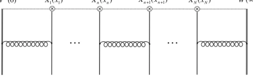
whereψ (x)=dln(x)/dx is the Euler digamma function. It is important to notice that this is not the form naturally coming from the computation of Feynman graphs contributing to the renormalization of(1.23). Namely, the one-loop light-cone Hamiltonians for interaction of GKP excitations among themselves are not sensitive to the boundary Wilson lines and thus have to enjoy fullSL(2,R)invariance[21,22]. They are shown in the middle graph inFig. 2. However,
Fig. 2. A representative Feynman graph defining the one-loop dilatation operator for theΠ-shaped operator(1.23)in the light-cone gauge. It corresponds to the sum of pair-wise Hamiltonians, i.e., with only two nearest-neighbor pairs of fields interacting with each other at a time. The vertical straight lines stand for the elementary fieldsXdescribing the GKP excitations, while the wavy lines represents gluons for the boundary interactions with the Wilson lines, or encode a sum of several diagrams for two adjacentXnXn+1inner fields. A diagram without field insertions is subtracted from the above diagrams to make the total contribution well defined.
it is not the case in the above form due to the presence of the logarithms. The latter emerge from 1/α-factor in the second integral in Eq.(1.26)that was introduced in order to match it to the boundary Hamiltonians(1.20), with all intermediate logarithms canceling telescopically with one another. Therefore, in order to restore the conformal symmetry property, one can shift the logarithms into the boundary terms, such that the reshuffled Hamiltonians will become
h01=ψ (1)−ψ (x1∂1+2s)−lnx1= −ln
x12∂1+2sx1
, hn,n+1=2ψ (1)−ψ (xn,n+1∂n+2s)−ψ (xn+1,n∂n+1+2s),
hN∞=ψ (1)−ψ (−xN∂N)+lnxN= −ln∂N, (1.28) withHN=h01+N−1
n=1 hn,n+1+hN∞. Here we used identity(B.6)fromAppendix Bto recast the boundary Hamiltonians in terms of logarithms. Notice that h01+h1∞=H01+H1∞ in agreement with(1.19).
At this point we would like to notice that similar Hamiltonians emerged in the discussion of the Regge limit of scattering amplitudes in Ref.[23].
Thus, the goal of this paper is to solve the spectral problem for the multiparticle Hamiltonian (1.24)
HNΨu(x1, . . . , xN)=EuΨu(x1, . . . , xN). (1.29) Its eigenenergies Eu determine the first quantum corrections to the propagation of the GKP excitations(1.9)as was exemplified for the octagon and decagon in Eqs.(1.8)and(1.13), re- spectively. The wave functionsΨu, on the other hand, determine multiparticle hexagon transition amplitudes,
Hs(u|v)∼ ΨvTs
g+ Ψu
, (1.30)
as a matrix element of a conformal transformation Ts(g+) with respect to a suitably defined scalar product that is defined later in this paper. We will establish its factorization in terms of single-particle leading-order hexagons that was conjectured and tested for specific N’s in Ref.[16]and the (inverse) single-particle measureμs(u)being related to the residue ofHs(u|v) atv=u[16].
The above problem (1.29)turns out to be integrable since the Hamiltonian HN possesses enough integrals of motion with eigenvaluesu=(u1, . . . , uN)to be exactly solvable. Thus we have the powerful machinery of integrable spin chain at our disposal for constructing the explicit
eigenfunctions and finding corresponding eigenvalues. For the case at hand, we are dealing with an open spin chain that does not possessSL(2,R)symmetry due to boundary interactions. In addition, as we can conclude from the one-particle eigenfunction(1.21), the system is not en- dowed with a vacuum states. As a consequence of this last fact, traditional methods based on the Algebraic Bethe Ansatz[24,25]are not applicable and instead one has to rely on the method of the BaxterQ-operator[26]and the Separation of Variables (SoV)[27].
Our subsequent consideration is organized as follows. After introducing in the next section a natural Hilbert space for the Hamiltonian and a scalar product that makes it self-adjoint, we find a complete set of integrals motion commuting withHN. As a next step on the way to solve the spectral problem, we recall the factorization ofR-matrices[24,25] into intertwiners that play a crucial role in our analysis. In Section3, we use them to construct the Hamiltonians and demonstrate their equivalence with the ones arising in the problem of renormalization of the light-cone operators(1.23). Then in Section 4, we construct the BaxterQ-operator as well as its conjugate making use of available techniques developed forSL(2)invariant magnets. Both operators are then used to generate commuting Hamiltonians. In Section5, we devise an iterative procedure to obtain the eigenfunctions of the Hamiltonian. We then cast them in a form of a contour integral representation as well as an integral representation in the upper half-plane. The latter is instrumental in demonstration of their orthogonality with respect to the scalar product introduced earlier. To adopt our consideration for multiparticle contributions to the null polygonal Wilson loops, we define a new scalar product on the real half-line in Section6and establish its relation to the one for the analytically continued functions in the upper half-plane. Then we explicitly compute the square and hexagon leading order transitions in Section 7, where we also prove the factorized ansatz for the latter suggested in Ref.[16]. Finally, we conclude by pointing applications of the current construction to the operator product expansion of polygonal Wilson loops and outline the generalization to include GKP excitations of different spins. Several appendices contain conventions and computational details that we found inappropriate to include in the main body of the paper. We also provided there a complementary construction the wave function in the representation of Separated Variables and its relation to the eigenvalues of the BaxterQ-operator.
2. Open spin chain
The Hamiltonian(1.24)defines a non-periodic one-dimensional lattice model of interacting spinsSn=(Sn0, Sn+, Sn−)acting at each site defined by the coordinate of the GKP excitation.
They form an infinite-dimensional representation of thesl(2,R)algebra, Sn+, Sn−
=2Sn0, Sn0, Sn±
= ±Sn±. (2.1)
Our choice of the representationSn±,0 for the spin generators S±,0 on the fields X is driven by the form of the pairwise Hamiltonians (1.28) acting on the elementary fields X(x), i.e.
[S±,0, X(xn)] =iSn±,0X(xn)[21,22]. They are taken in the form of differential operators act- ing on lattice sites
Sn+=x2n∂n+2sxn, Sn−= −∂n, Sn0=xn∂n+s, (2.2) where all labels of the representation s are the same for anyn. The latter condition defines a homogeneous open spin chain. The spin variables is assumed to be real and bounded from below by 1/2.
2.1. Scalar product
It is convenient to define a scalar product on the space of functionsΨu(x1, . . . , xN). Its choice is a matter of convenience but it has to be adapted to the physical problem under consideration.
As was explained in Section1, we are interested in theτ-dependence of correlation functions of the light-cone operatorsONwhich read schematically
0|ON
x1, . . . , xN
eaτHNON(x1, . . . , xN)|0
=
u
eaτ Eu Ψu
x1, . . . , xN†
Ψu(x1, . . . , xN). (2.3)
Here the functionsΨuare determined by the operator matrix elements between the eigenstate
|Euof Hamiltonian and the vacuum,8Ψu(x1, . . . , xN)= Eu|ON(x1, . . . , xN)|0, and the sum runs over all eigenstates. Although the variablesxnare the light-cone coordinates of the fieldsX entering the Lagrangian of the theory and are, therefore, real, nevertheless distribution amplitudes Ψu(z1, . . . , zN)can be regarded as functions ofzn in complex plane. It is known that they are analytic functions in upper half-plane and vanish at infinity. As a consequence of this change, the sl(2,R)generators in Eq.(2.2)depend and act on theznvariables accordingly.
In what follows we will consider the spectral problem (1.29)on the space of functions of N complex variablesznanalytic in the upper half-plane and endowed with a standardSL(2,R) invariant scalar product[28]. Such a formulation appeared to be very useful for constructing the SoV representation for the closed and openSL(2,R)spin chains[29,30]. The scalar product on the space of functions holomorphic in the upper half-plane9is defined as follows[28]
Φ|Ψ =
Dzn Φ(zn)∗
Ψ (zn), (2.4)
wherezn=xn+iyn. The integration measure reads Dzn=2s−1
π dxndyn(2yn)2s−2θ (yn) (2.5)
and the integration runs over the upper half-plane due to the presence of the step-functionθ (yn).
Under this scalar product the generators(2.2)are anti-self-adjoint Sn0,±†
= −Sn0,±, (2.6)
with hermitian conjugation defined conventionally as Φ|GΨ =
G†ΦΨ
. (2.7)
The Hilbert space of the model is given by the tensor product of Hilbert spaces at each site N
n=1Vn, such that the generalization of the scalar product(2.4)to multivariable functions is straightforward,
Φ|Ψ = N
k=1
Dzk
Φ(z1, . . . , zN)∗
Ψ (z1, . . . , zN). (2.8)
8 In QCD terminologyΨu(x1, . . . , xN)is known as the distribution amplitude.
9 The Hilbert spaces of holomorphic functions are well studied mathematical topic, for a review, see Ref.[31].
One can immediately verify that the HamiltonianHNis a hermitian operator
H†N=HN (2.9)
by virtue of Eq.(2.6). Notice that this is obvious for the boundary Hamiltonians(1.28)that are merely functions of the spinS±generators acting on the right/left-most sites. These Hamiltonians are notSL(2,R)invariant. The intermediate Hamiltonians can be cast in anSL(2,R)symmetric form[32]and read
hn,n+1=2ψ (1)−2ψ (Jn,n+1). (2.10)
HereJn,n+1is an operator related to the two-particle Casimir via the formula
Jn,n+1(Jn,n+1−1)=(Sn+Sn+1)2. (2.11)
These are explicitly self-adjoint. In the following section, we show that there exists a complete set of integrals of motion (commuting with the Hamiltonian) that are hermitian with respect to this scalar product and thus their eigenstates form an orthogonal set.
Closing this section we remark that to any operatorAacting on the Hilbert space(2.8)we can associate a functionAofN holomorphic andN anti-holomorphic variables, i.e., the so-called integral kernel, in a unique way via the relation
[AΨ](z1, . . . , zN)= N
k=1
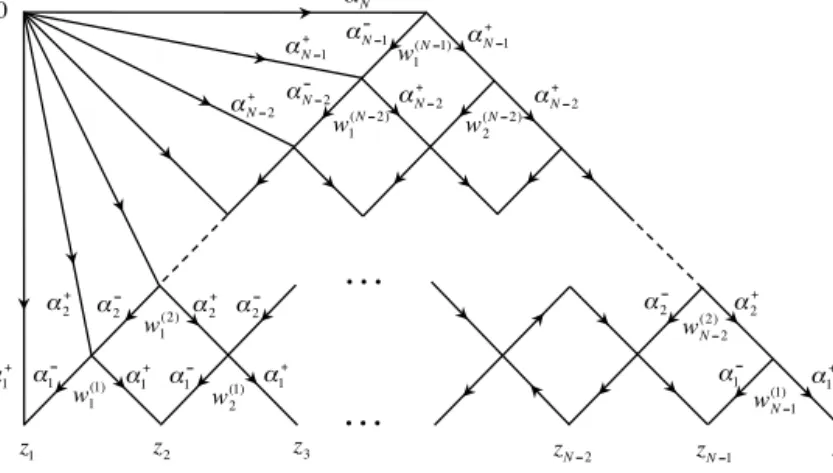
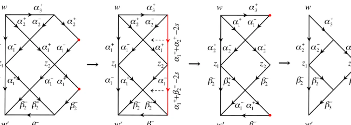
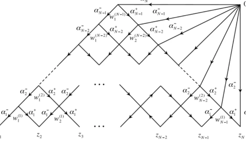
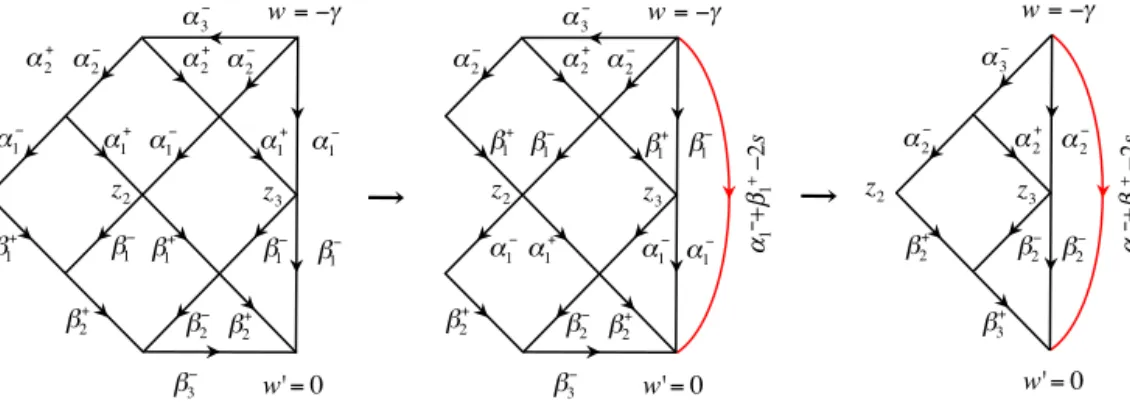
DwkA(z1, . . . , zN| ¯w1, . . . ,w¯N)Ψ (w1, . . . , wN). (2.12) It turns out that integral kernels of operators which we construct in the following sections take a form of two-dimensional Feynman diagrams. All operator identities can be cast into the identities between Feynman diagrams which can be verified with the help of a standard diagram technique that we remind inAppendix B.
2.2. Integrals of motion
We start the construction of the integrals of motion following the conventional R-matrix approach[24,25]. The Lax operator acting on the direct productC2⊗Vn of an auxiliary two- dimensional spaceC2and the quantum space at then-th siteVnis defined as
Ln(u, s)=u+i(σ·Sn)=
u+iSn0 iSn− iSn+ u−iSn0
, (2.13)
with a complex spectral parameteru. We also displayed its dependence on the spin parameters.
The product ofNcopies of this operator in the auxiliary space determines the monodromy matrix T(s)(u),
T(s)N(u)=L1(u, s)· · ·LN(u, s)=
AN(u) BN(u) CN(u) DN(u)
(2.14) with its elements acting on the quantum space of the chainN
n=1Vn. As can be easily established from the Yang–Baxter equation with a rational R-matrix [24,25], each element of the mon- odromy matrix commutes with itself for arbitrary spectral parameters, i.e.,[DN(u), DN(v)] =0 etc. As we will demonstrate below, the operatorDN(u) commutes also with the Hamiltonian (1.24)
DN(u),HN
=0. (2.15)
It can be easily seen from the form of the Lax operator that the entries of the monodromy matrix are polynomials of degreeN in the spectral parameter uwith operator valued coefficients. In particular,
DN(u)=uN+ ˆd1uN−1+ · · · + ˆdN. (2.16) The expansion coefficients (integrals of motions)dˆk,k=1, . . . , N, commute with each other and with the Hamiltonian,[ ˆdk,dˆn] = [ ˆdk,HN] =0. Their eigenvalues define a complete set of quan- tum numbers of the eigenstate. Since the eigenvalues of the operatorDN(u)are polynomials in u, its eigenstates can be labeled by the zeroes of the corresponding polynomial,u=(u1, . . . , uN)
DN(u)Ψu(z1, . . . , zN)= N n=1
(u−un)Ψu(z1, . . . , zN)
= N n=1
(u− ˆun)Ψu(z1, . . . , zN). (2.17) Here the operatoruˆn are the so-called Sklyanin’s operator zeroes[27], defined by the relation
ˆ
ukΨu=ukΨu.
As follows from Eq.(2.13), the integrals of motiondˆnare polynomials in the spin generators Sn(n=1, . . . , N), for instance,
dˆ1= −i
S10+ · · · +SN0
, (2.18)
with the restdˆnbeing given byn-th order differential operators. Thus, Eq.(2.17)defines a system ofNdifferential equations that once solved yields the eigenfunctions of the open spin chain. By virtue of the property(2.6), the operatorDN is self-conjugate (for realu) and thusdˆn(and as a consequenceuˆn) are hermitian as well. This implies that all eigenvaluesunare real.
3. FactorizedR-matrices and Hamiltonians
Let us now demonstrate that local Hamiltonians, arising from theR-matrices acting on the direct product of two copies of the quantum spaceV⊗V, indeed coincide with the one coming from diagrammatic calculations alluded to in Section1.2.
3.1. Intertwiners
To start with let us recall relevant facts about the aforementioned quantumR-matrices. Let us represent theR-matrix in the formR12=Π12Rˇ12, whereΠ12 is a permutation operator on the product of two spaces, Π12Ψ (z1, z2)=Ψ (z2, z1). For the operator Rˇ12 the conventional RLL-relation[24,25]takes the following form
Rˇ12(u−v)L1(u, s1)L2(v, s2)=L1(v, s2)L2(u, s1)Rˇ12(u−v). (3.1) HereL1(2)are the differential operators inz1(z2), according to their expression(2.13)continued in the upper half-plane. In the above equation, we have clearly displayed all parameters which these operators depend on (notice that we will not assume in this section thats1=s2). Eq.(3.1) shows that the operatorRˇ12interchanges the parameters of the Lax operators acting on the first and the second spaces,(u, s1)↔(v, s2).
Making use of the explicit form of the generators it is possible to demonstrate that the Lax operator can be factorized into a product of triangular matrices
Ln(u, sn)=
1 0 zn 1
u+isn−i −i∂n
0 u−isn
1 0
−zn 1
. (3.2)
As it is obvious from this representation, it is convenient to introduce the following combinations of the spectral parametersu,vand the spinss1,s2
u±=u±is1, v±=v±is2, (3.3)
such thatL1(u, s1)≡L1(u+, u−)andL2(v, s2)≡L2(v+, v−). As Eq.(3.1)suggests, the opera- torRˇ interchanges simultaneouslyu±withv±.
A fruitful approach to solving Eq.(3.1)was pioneered in Ref.[33]. It was suggested there to look for the solution of Eq.(3.1)in the form of a product of two operators
Rˇ12(u−v)=R+12(u+|v+, u−)R−12(u+, u−|v−), (3.4) that exchange corresponding spectral parameters(3.3)independently, i.e.,
R+12(u+|v+, v−)L1(u+, u−)L2(v+, v−)=L1(v+, u−)L2(u+, v−)R+12(u+|v+, v−), (3.5a) R−12(u+, u−|v−)L1(u+, u−)L2(v+, v−)=L1(u+, v−)L2(v+, u−)R−12(u+, u−|v−).
(3.5b) These operators change the spin of thesl(2,R)representations and map the Hilbert spaces of the spin chain sites as follows
R+12(u+|v+, v−):Vs1⊗Vs2→Vs1−i(v+−u+)/2⊗Vs2+i(v+−u+)/2, (3.6a) R−12(u+, u−|v−):Vs1⊗Vs2→Vs1+i(v−−u−)/2⊗Vs2−i(v−−u−)/2, (3.6b) where we explicitly displayed the parameters labeling the representation. The solution for inter- twiners was found in Ref.[33]and they read
R+12(u+|v+, v−)=(z21∂2+iv−−iu+) (z21∂2+iv−−iv+)
(iv−−iv+)
(iv−−iu+), (3.7a)
R−12(u+, u−|v−)=(z12∂1+iv−−iu+) (z12∂1+iu−−iu+)
(iu−−iu+)
(iv−−iu+), (3.7b)
wherez12=z1−z2. These can also be easily cast in the integral form making use of the definition of the Euler Beta function. Note also that the operatorsR±12 depend only on the difference of spectral parameters, i.e.
R+12(u+|v+, v−)=R+12(0|v+−u+, v−−u+),
R−12(u+, u−|v−)=R−12(u+−v−, u−−v−|0). (3.8)
3.2. Hamiltonians
The localSL(2,R)invariant Hamiltonians arise as coefficients of the leading power in the ex- pansion of theR-matrix in Taylor series in the vicinity ofu−v=ε→0[32]. The representation in terms of the Euler Gamma functions(3.7a)and(3.7b)then yields,
R+12(u+|v+, v−)=1−iεh+12+O ε2
, (3.9)
R−12(u+, u−|v−)=1−iεh−12+O ε2
, (3.10)
where
h+12=ψ (2s)−ψ (z21∂2+2s), h−12=ψ (2s)−ψ (z12∂1+2s). (3.11) Comparing their sum h12=h+12+h−12+2(ψ (1)−ψ (2s))with the intermediate Hamiltonian (1.28), we immediately find that they coincide up to an additive constant. The commutation relation of these Hamiltonians with the monodromy matrix(2.14)can easily be established from the Yang–Baxter equations(3.5a)and(3.5b)for the intertwining operators by expanding both sides around the pointv=u−εasε→0. We get forO(ε)terms
h±12,L1(u, s)L2(u, s)
=iM±1L2(u, s)−iL1(u, s)M±2, (3.12) where
M+n =
1 0 zn 0
, M−n =
0 0
−zn 1
. (3.13)
ForN-site Hamiltonians, the commutation relations with the monodromy matrix can be estab- lished from the above equations(3.12)to be
N−1
n=1
h±n,n+1,T(s)N(u)
=iM±1L2(u, s)· · ·LN(u, s)
−iL1(u, s)· · ·LN−1(u, s)M±n. (3.14) There are leftover boundary terms in the above equations which have to be canceled against some boundary Hamiltoniansh01 andhN∞to enforce the commutativity. We are going to find their form next. To project out the DN(u) entry from the monodromy matrix, one sandwiches the above commutation relations between the two-dimensional vector |↓ =(0,1)T and its trans- posed ↓| =(0,1). These equations in turn can be reduced to a set of local equations for the boundary Hamiltonians, namely,
↓| h±01,L1(u, s)
= −i↓|M±1, h±N∞,LN(u, s)
|↓ =iM±N|↓. (3.15) They receive the following solutions
h+01= −ψ (z1∂1+2s), h−01= −lnz1, h+N∞=0, h−N∞= −ln∂N. (3.16) Summing these expressions up, we recognize the boundary Hamiltonians(1.28) that emerged from the gauge theory analysis (again up to an additive constant). Thus, finding the eigenfunc- tions of the Hamiltonian is equivalent to the diagonalization of the operatorDN(u), which we address in Section5below.