Relativistic quantum mechanics

(1)

Zusammenfassung

Das Ziel dieser Arbeit ist die Untersuchung der Abstrahlung korrelierter Photonen durch zeitweise beschleunigte Ladungstr¨ager. Desweiteren untersuchen wir die Korrelationen dieser Photonen, d.h.

wir betrachten die Verschränkung zwischen den abgestrahlten Photonen. Um dieses Ziel zu er- reichen entwickeln wir ein Rahmenwerk der skalaren und spinoriellen Quantenelektrodynamik in einem linearen, homogenen und endlich ausgedehnten klassischen elektrischen Hintergrundfeld. Als erstes konstruieren wir die Lösungen der zugehörigen relativistischen Wellengleichungen und benutzen diese Lösungen um die Materiefelder zu quantisieren. Durch die Wirkung des elektrische Hintergundfeldes kann das Vakuum nicht eindeutig definert werden. Das kann als Instabilität des Vakuumss interpretiert werden, was bedeutet, dass Elektron-Positron-Paare entstehen und somit der Teilchen-Inhalte eines Zustands wächst. Die resultierende Rate der Elektron-Positron-Paarerzeu- gung wird in der Mitte dieser Arbeit betrachtet. Im Hauptteil dieser Arbeit leiten wir Ausdrücke für die Streumatrix-Elemente der Photonenabstrahlung durch geladene Teilchen in erster und zweiter Ordnung Störungstheorie her. Für die erste Ordnung benutzen wir eine ultrarelativistische Nährung um geschlossene analytische Ausdrücke für die Wirkungsquerschnitte herzuleiten. Wir zeigen, dass es, im Widerspruch zu den klassischen Ergebnissen, bei der Abstrahlung von Photonen durch Elec- tronen, aufgrund des Spins, im Allgemeinen keinen blinden Fleck in der Beschleunigungsrichtung gibt. Zuletzt untersuchen wir noch die Korrelationseigenschaften der durch beschleunigte Electronen abgestrahlten Photonen in zweiter Ordnung Störungstheorie. Wir stellen fest, dass Photonenpaare in ihren Polarisationsfreiheitsgraden maximal verschränkt sind, wenn sie in Beschleunigungsrichtung

(4)

abgestrahlt werden und, dass sie sich n¨ahrungweise in einem Produktzustand befinden, wenn die beiden Photonen in ein und dieselbe Richtung senkrecht zur Beschleunigungsrichtung abgestrahlt werden.

(5)

Abstract

The aim of this thesis is to investigate the emission of correlated photons from transiently accelerated charges. Furthermore, we want to investigate the correlations of such photons, with other words entanglement. To reach this goal we develop a framework of scalar and spinor quantum electrodynamics in a classical, electric background field which is linear, homogenous and finite extended. First of all we construct the solutions of the corresponding relativistic wave equations and use these solutions to quantize the matter fields. Due to the presence of the electric field the vacuum state cannot be defined unambiguously. This can be interpred as an unstability of the vacuum which means that electron-positron pairs emerge and thus the particle content of a state increases. The resulting rate of electron-positron pair production is investigated in the middle of this thesis. In the main part of this thesis we derive expressions for the scattering matrix elements of photon emission from charged particles in first and second order perturbation theory. For the first order we use an ultrarelativistic approximation to derive closed analytic expressions for the cross section. We show that, due to the spin, there is not a blind spot for photon emission from electrons in the acceleration direction in general. Finally we investigate the correlation properties of emitted photon pairs in second order perturbation theory. This result contradicts the results of classical electrodynamics. Moreover, we find that emitted photon pairs are maximally entangled in their polarization degrees of freedom if they are emitted in the acceleration direction and that they are approximately in a product state if both photons are emitted in the same direction perpendicular to the acceleration direction.

(6)

Chapter 1 Introduction

Does a linearly accelerated charged particle radiate and, if it does, what are the properties of the arising radiation? Classical electrodynamics gives a clear answer to this question: Linearly accelerated particles radiate and the angular distribution of this radiation is given by the relativistic Larmor formula [1]

dP

dΩ = e²x˙² 4πc³

sinθ²

(1− ^x_c^˙ cosθ)⁵. (1.1)

However, the classical description of the interaction between the electromagentic field and matter is in many experimental and technical relevant situations not adequate, it must be replaced by a quantum mechanical description. The state of the art method for describing electrodynamical phenomena in the framework of quantum theory is Quantum Optics. How does Quantum Optics answer our question? At the first glance the answer is, again, the Larmor formular [2]. If one then goes one step further in the accuracy of the calculations and considers the back reaction of the emitted photon on the charged particle one gets the simultanious emission of two photons; a photon pair. Due to the quantum properties of the electromagnetic field the correlations between these photons can be much stronger than classical correlations, i.e. the photon pair is entangled to some degree [3]. Hence accelerated electrons could be a source of entangled photon pair radiation

(7)

with energy in the keV domain. This could be of enormous value for experiments in Quantum Optics and experimental Quantum Information [4]. In Quantum Optics all these results are derived while assuming the accelerated charged particle to be simply a classical point particle without any inner degree of freedom - like spin. In contrast to this model the charged particles that are used in most of the experimental cases have spin and thus the quantum optical description outlined above can only be adequate to some extent since effects caused by the spin are neglected. In Quantum Optics one deals with such inner degrees of freedom by modelling them as ann-level system, that is a harmonic oscillator with n levels with an appropriate coupling to the external electromagnetic field [2]. By investigating a quantum optical model for an uncharged particle with inner degrees of freedom we arrive at the following statement: If such a particle is in the ground state and is then accelerated, there is a finite probability that it will be found in an excited state after the acceleration; the energy spectrum of the excitation probability is thermal, that is the occupation probabilities of the energy eigenstates of the n-lever system undergoing an acceleration a are the same as if the system were coupled to a thermal bath with temperature kT = _2πc^!^a. This theoretical prediction is called the Unruh effect [5] and has been thoroughly investigated in several publications by different authors although it has not yet been experimentally observed. It can be interpreted as the statement that for non inertial observers the quantum vacuum is ambigious, i.e. the particle content of the environment depends on the acceleration [6]. In this way the Unruh effect is closely related to the Hawking effect for black holes [7]. Obviously we must also consider the Unruh effect for a charged accelerated particle with inner degrees of freedom in the calculations¹.

We see that the quantum optical description of an accelerated charged particle explains most of the corresponding macroscopic phenomena but is insufficient if one wants to take a closer look.

Quantum Electrodynamics is, in contrast, a theory that deals with electrons and their interaction with the electromagnetic field in a highly precise way. In this theory both the electromagnetic field and matter are treated in second quantization, thus all the quantum mechanical properties corresponding

(8)

to space and momentum of photons and massive charged particles are accessible which allows the investigation of entanglement within these variables. A further great advantage of this theory is that the spin is completely inherent because we describe the electron as an excitation of a spinor field;

no artificial inner degrees of freedom have to be established like in Quantum Optics. Furthermore, instead of giving the charged particle a fixed trajectory, as it is done in most of the quantum optical approaches in QED, the acceleration is achieved by an external electric field and all recoil effects due to photon emission processes are included. In this thesis we show that these advantages lead to significant differences in the predictions of the photon emission probability in contrast to predictions given by Quantum Optics. This is relevant especially in experiments geared towards the detection of photon pair radiaton, like those described in ref. [4]. Our results show that it is questionable that the quantum optical description used in ref. [3] and [4] to describe these experiments is sufficient.

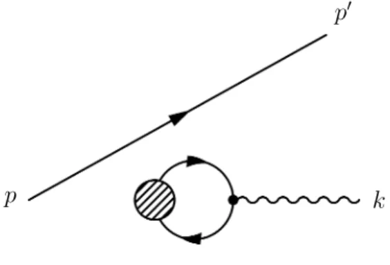
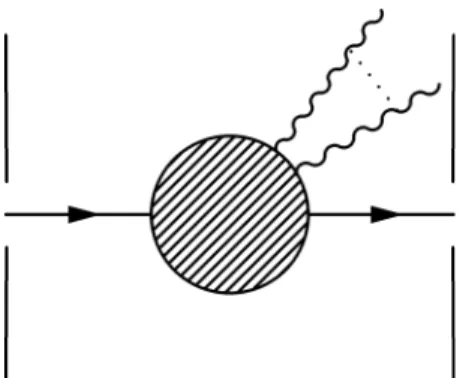
Unfortunately in QED the effects of the interaction between the matter field and the electromagnetic field can, in most cases, only be calculated in a perturbative way, order by order. Because of this QED is mainly used for the calculation of cross sections of processes with only a few particles in Minkovski space. To succesfully model the acceleration of a particle in this perturbative framework and to investigate the emission of photons from an accelerated particle it is necessary to consider processes of very high order. This is hardly a solvable problem. However, we can model the acceleration of particles approximately if we use a classical, linear electric background field and negelect the backreaction of the charged particle on this background field. Radiation can be considered by splitting the electromagnetic field into the classical background field that accelerates the charged particles and a quantum mechanical radiation field. In ref. [9] the authors use this framework in first order perturbation theory to investigate the emission of photons from infinitely, uniformly accelerated electrons. In this thesis we use the framework of QED to investigate the emission of photons from charges that are transiently accelerated by a linear finite extended electric field like that which can easily be realized in a plate capicitor (see figure 1.1). Furthermore we investigate the correlations of the emitted photons in second order perturbation theory.

(9)

Figure 1.1: Charged particle accelerated by the electric field of a plate capacitor interacting with the electromagnetic field.

In chapter 2 we derive the solutions of the relativistic wave equations for scalar and spinor particles in a classical finite extended electric field and investigate the propagation of wave packets. In chaper 3 we outline the procedure of second quantization and construct the many particle quantum theory for scalar and spinor particles in an external field. In chapter 4 we discuss the instability of the vacuum and the pair creation rate. The central part of this thesis is chapter 5. We use the developed many particle quantum theory of scalar and spinor particles and their interaction with the electromagnetic field to derive the probability of photon emission by transiently accelerated charges in first and second order perturbation theory. In section 5.4 of this chapter we discuss the correlations between emitted photon pairs in second order perturbation thory. In chapter 6 we give conclusions and an outlook on potential further work.

(10)

Chapter 2 Relativistic quantum mechanics

In relativistic quantum mechanics a scalar or spinor particle can be modelled as a wave packet of the solutions of the Klein-Gordon or Dirac equation respectively. Acceleration can be brought into play by coupling the wave equations minimally to a linear electric field. In the next two subsections we calculate the solutions of the relativistic wave equations coupled to a finite extended linear electric field. For the scalar particle we additionally derive ultrarelativistic approximations of the solutions of the wave equation, compare them with the corresponding WKB solutions and investigate the propagation of wave packets in this electromagnetic background field.

2.1 Scalar particles

2.1.1 Solutions of the wave equation

The Klein-Gordon equation is

!

D^µDµ+ m²c²

!²

"

Φ = 0 (2.1)

whereDµ=∂µ+i_!^qAµ and the inner product on Minkowki space is

ηµν =diag(1,−1,−1,−1). Aµ is the electromagnetic four-vector potential and m is the mass of the scalar particle. We decide to describe electrons as particles and positrons as antiparticles, thus we

(11)

haveq =−e. We consider the following four-vector potential illustrated in figure 2.1:

A0 =











x3,0E/c : x3 < −x3,0

−x3E/c : −x3,0 ≤ x3 ≤ x0,3

−x3,0E/c : x3,0 < x3

(2.2)

and Aµ = 0 for µ#= 0.

I

!

"

0 0 A0

x3

−x3,0

II

######

x3,0

III

1 2 3

Figure 2.1: A diagram of the potential −eA0. It can be separated into three spacial sections I, II and III with different solutions of the wave equation (2.1) and into three energy domains 1, 2 and 3 with different particle and antiparticle content. Section 1: cp₀ < −eEx_3,0, Section 2:

−eEx3,0 ≤cp0 ≤eEx3,0, Section 3: eEx3,0 < cp0.

Now we devide the domain of Φ, i.e. the x3-axis into three sections corresponding to the three sections of the potential I, II and III and make the ansatz

Φ(x, t) := φ(x3)e^!ⁱ^p^⊥^x^⊥e⁻ⁱ^p^!⁰^ct (2.3)

where p_⊥ is the part of the vector p lying perpendicular to the x3 direction. By defining m²_⊥c² :=

m²c²+p²_⊥ we get three ordinary linear second order differential equations in x3. Section I (x3 <

−x3,0)

(12)

Section II (−x3,0 ≤x3 ≤x3,0) d²φII

dx²₃ + (p0−eEx3)²

c²!² φII −m²_⊥c²

!² φII = 0 (2.5)

Section III (x_3,0 < x₃)

d²φIII

dx²₃ +(p0−eEx3,0)²

c²!² φIII − m²_⊥c²

!² φIII = 0. (2.6)

For the sake of simplicity we define new dimensionless variables and parameters.

˜

p0 :=' _c

2eE!p0 p˜_⊥ :=' _c

2eE!p_⊥ z :=(

2eE!c x3

˜t:=(

2eE!c ct µ²_⊥:= _2eE^m²^⊥^c_!⁴_c

(2.7)

To get a feeling for these dimensionless variables we give some experimentally relevant values: for E = 10⁶^!_!^V_m, x3,0 = 10⁻⁵!m and p_⊥ = 0 we find z0 = 3.65×10⁶ and µ_⊥= 7.4×10⁵.

With the definitions (2.7) the differential equations (2.4), (2.5) and (2.6) become Section I (x3 <−x3,0)

d²φI

dz² + (˜p0+z0/2)²φI−µ²_⊥φI = 0 (2.8) Section II (−x3,0 ≤x3 ≤x3,0)

d²φII

dz² + (˜p0 −z/2)²φII −µ²_⊥φII = 0 (2.9) Section III (x3,0 < x3)

d²φIII

dz² + (˜p0−z0/2)²φIII −µ²_⊥φIII = 0 (2.10) For sections I and III the solutions are straight forward. For section II we make a additional

(13)

transformation to ˜z :=e⁻ⁱ³⁴^π(z−2˜p0) :=γ(z−2˜p0) and get with the definition n:=iµ²− ¹₂ d²φII

d˜z² + )

n+ 1 2− z˜²

4

*

φII = 0. (2.11)

This is the parabolic cylinder equation known from harmonic analysis. A special complete set of solutions consists of the so-called parabolic cylinder functions Dn[˜z] and Dn[−z] [10]. We use these˜ solutions due to their asymptotic properties, which appear appropriate for the following interpretation as in- and out-propagating particle and antiparticle states like it is done in [11], [12] and [13]. Doing this we arrive at the following general solutions: Section I (x3 <−x3,0)

φI(z) =a1e⁻^i˜^p(⁻^)z+b1e^i˜^p(⁻^)z (2.12)

Section II (−x3,0 ≤x3 ≤x3,0)

φ_II(z) =AD_n[γ(z−2 ˜p₀)] +BD_n[−γ(z−2 ˜p₀)] (2.13)

Section III (x3,0 < x3)

φIII(z) = a2e⁻ⁱ^p(+)z^˜ +b2eⁱ^p(+)z^˜ (2.14) where ˜p(−) = ((˜p0 + ^z₂⁰)² −µ²_⊥)¹² and ˜p(+) = ((˜p0 − ^z₂⁰)² −µ²_⊥)¹² and the factors a1, b1, a2, b2, A and B must be specified by connection conditions between the three sections of the wave function’s domain and by the interpretation as in- and out-propagating states.

In the next step we have to fix the free parameters in equations (2.12) to (2.14). Since the Klein-Gordon equation is a second order differential equation and the potential Aµ is continuous, the solutions φ for the whole domain have to be twice continuously differentiable, i.e. φ ∈ C₂^∞(R).

These connecting conditions give us four equations.

(14)

φ^$_I(−z0) = φ^$_II(−z0) φ^$_II(z0) =φ^$_III(z0)

where the prime indicates the derivative with respect to z. We can now fix the two remaining free parameters by normalization of the wave functions and, at this point, everything is fixed by physical and mathematical constraints. The last parameter, however, can only be fixed by the identification of in- and out-propagating states and this is totally ambigious. In literature we find two different approaches to identify in- and out-propagating states; one is followed by ref.[14] and the other by ref.[15] and [16]. They are illustrated by the diagrams in figures 2.2 and 2.3. Both identification schemes are based on a wave packet picture, i.e. by investigation of the group velocity vg =c_p_˜ ^p^˜

0+^z₂⁰

of a wave packet constructed from these wave functions. The identification scheme of ref. [14]

can be summarized by the statement: an in-propagating state from the left is a state with no in- propagating wavepacket from the right and analogous for in-propagating states from the right and out-propagating states. Similary the identification scheme of ref. [15] can be summarized by the statement: an in-propagating state from the left is a state without out-propagating wave packet on the left and analogous for the other states. We find that the transformation that connects the two schemes is CPT, i.e. the subsequent application of time reversal, point reflection (parity) and charge conjugation. There is no argument for ruling out one of these identification schemes or any other identification scheme using linear combinations of the wave functions constructed with the identification scheme of ref. [14] and ref. [15]. Nevertheless, in the following we construct the left and right in-propagating states in the scheme of ref. [14] only since, in the context of the one particle theory, it seems more natural that the incident particle is reflected than that it is annihilated by a particle coming from the right. The corresponding out-propagating states can be obtained by complex conjugation of the spatial part of the wave function. This can easily be seen by looking at the exponential form of the wave functions in section I and III of the z-axis, which indicates that complex conjugation flips the sign of the group velocity.

To construct the wave functions we start with the investigation of the group velocity. For an

(15)

(in left)

##

$$ ##

##%

$$

& ##%

(out left)

##

$$

##% $&$

$$

&

(in right)

$$

$$ ##

$$

&

$$

& ##%

(out right)

##

$$

##% $&$

##%

Figure 2.2: A diagram of the identification scheme of ref. [14]. The vertical line represents the source of reflection, i.e. the electromagnatic fild.

(in left)

##

$$

##% $&$

##%

(out left)

$$

$$ ##

$$

&

$$

& ##%

(in right)

##

$$

##% $&$

$$

&

(out right)

##

$$ ##

##%

$$

& ##%

Figure 2.3: A diagram of the identification scheme of ref. [15].

in-propagating state from the left the group velocity has to be positive on the left. One can easily see that the sign of vg depends on the energy range. Thus we have to split the energy range into three domains as it is shown in figure 2.1. We name the domains 1, 2 and 3 under barrier regime, pair creation regime and over barrier regime respectively. The reason for denoting domain 2 as pair creation regime will become clear in the following. Due to the ansatz (2.3) we define the wave functions

Φ^(p,a)_in,p(_±₎ :=φ^(p,a)_in,p(_±₎e^ip^⊥^x^⊥⁻^ip^(p,a)⁰ ^(p(^±^),p^⊥^)t. (2.15) The explicit expressions for the functions φ^(p,a)_in,p(_±₎ are given in the appendix 7.2. We term states as particle ^(p) and antiparticle ^(a) states due to their asymptotic charge density, here and in the following the indices p(+) and p(−) denote a left or right state respectively. The charge density for Klein Gordon fields is given by

(16)

Since the covariant derivative D0 depends only on x3 we can restrict our investigations to one di- mension and get

ρ[φ](z) = −e(p0−eA0(z))φ^∗(z)φ(z). (2.17) Thus the density is negative forp0 > A0(z) and positive for p0 < A0(z). Since we are only interested in a definition of states in the asymptotic regime where z → ±∞ we term the left(right) states with negative charge density on the left(right) side of the potential barrier as particle statesφ^(p)_in,p(−) and the left(right) states with positive charge density on the left(right) side as antiparticle states φ^(a)_in,p(−). Obviously this definition corresponds to the three energy domains. We obtain that particle and antiparticle states coexist only in the energy domain 2. Since this leads to an unstable vacuum state this domain is termed pair creation regime.

The next task is to investigate the normalization and orthogonality of the wave functions. For this purpose let us define the Klein-Gordon inner product which is, up to a factor e, equivalent to the charge, that is the intergral over the charge density (2.16).

(Φ1,Φ2)KG =−i +

d³x(Φ^∗₁D0Φ2−(D0Φ1)^∗Φ2). (2.18)

In ref. [14] the author sketches a proof for the orthogonality of the functions constructed with the above method with respect to the Klein Gordon inner product, i.e.

(Φ^(p,a)in,out,p(±),Φ^(p,a)_in,out,p_"_(±))_KG =(_p,a2π!δ(p(±)−p^$(±))(2π!)²δ⁽²⁾(p_⊥−p^$_⊥)

(Φ^(p,a)_in,out,p(₋₎,Φ^(p,a)_in,out,p_"₍₊₎)KG = 0

(2.19)

where(_p =−1 and (_a = 1.

It will be outlined in chapter 3 that these are the required properties of the solutions of the wave function to get a well defined quantum field theory. However, to calculate these properties explicitly, one has to show that the coefficients in (7.5) in the appendix are uniformly continuous over the

(17)

whole energy axis and one has to take into account that the expressions in (2.19) are generalized functions and thus have to be smeared out with test functions. We give an extended version of the proof of ref. [14] using these insights in the appendix of this work.

2.1.2 Ultrarelativistic approximation

In this section we derive the asymptotic properties of the solutions of the Klein-Gordon equation for large energies in the over barrier regime. The comparison with the WKB solutions of equation (2.1) in the same limit shows equivalence up to a phase and a normalization constant.

The WKB solution of (2.1) can be found with the help of ref. [17]. We restrict our considerations to the lowest order and neglect all reflection terms. For an in-propagating state from the left we find

φW KB(z) =

'p(−)

'κp(z)e^!ⁱ^R⁻^z^z⁰^dσκ^p^(σ)e⁻^ip(⁻^)z⁰ (2.20)

where κp(x3) = (

(¯p0 −^z₂)²−µ²_⊥. There is clearly an unspecified phase in this wave function due to the starting point of the integral in the argument of the exponential function. It can be fixed by asymptotic connecting conditions. Here we require the coincedence of the wave function with a plane wave moving from left to the right at the boundary of the acceleration region z = −z0. This corresponds to the identification scheme of ref. [14]. In section II of the z-axis and for large values of p0 equation (2.20) can be approximated by

φW KB(z)≈

'p(−)

√2¯p₀−z

√2e⁻ⁱ⁴^(2¯^p⁰⁻^z)²e^iµ²^⊥^ln(2¯^p⁰⁻^z)e⁴ⁱ^(¯^p⁰^+z⁰⁾²e⁻^iµ²^⊥^ln(2¯^p⁰^+z⁰⁾e⁻²ⁱ^z⁰^(2¯^p⁰^+z⁰⁾. (2.21)

We now investigate the same limit for the exact solutions we constructed in the last chapter with the identification scheme of ref. [14]. Up to a constant factor we get the same result with the identification scheme of ref. [15]. From equation (7.5), (7.2) and (7.1) in Appendix B we obtain that B(c ) ≈ ⁿc (c )e^ip(+)z D [−γ(2¯p −z )] ∝ (2¯p −z )⁻³ is strongly decreasing if ¯p → ∞ and

(18)

A(cL) ≈ _k¹c2(cL)e^ip(+)z⁰Dn−1[γ(2¯p0 −z0)] ∝ (2¯p0−z0)¹² increases. Thus we only have to calculate A(b1). For large ¯p0 we get with equation (7.1) in the appendix up to the normalization constant b1

again equation (2.21). This shows directly the correspondence between the semiclassical approximation and the identification schemes of ref. [14] and ref. [15] and all of their linear combinations. The complex phase can be adjusted by changing the starting point of the integration in the exponent in equation (2.20).

2.1.3 Propagation of wave packets

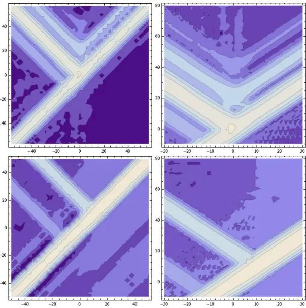
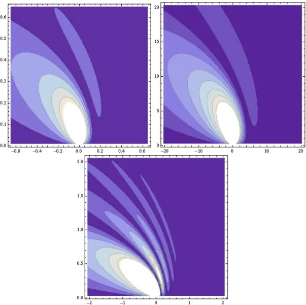
In this section we investigate the propagation of a wave packet in the causal identification scheme of ref. [14]. In what follows we present the results of numerical simulations computed withMathematica 6. In figure 2.4 we have plotted the logarithm ot the wave functions absolute value of in-propagating wave packets in the pair creation and over barrier regime. The system parameters lie above a critical value for pair creation; the Schwinger limit[18]. At this value the interaction with electron-positron field results in a quantum correction term for the energy momentum tensor of the electromagnetic field in the order ₁₀¹ with respect to the classical value. It is given by

Ecrit = ,

45 20

m⁴c⁵

!³ 1

α²(0 ≈10¹⁹V

m. (2.22)

In figure 2.4 one can clearly see the in-propagating packet and the two out-propagating packets;

one of the latter with enhanced amplitude. Further interesting features are the small packets on either side of the main packets. These features seem to form at the kinks of the potential located at

±z₀, i.e. they are results of an additional reflection. In contrast to the reflection effect known from optics, which arises from a discontinuity in the particle momentum, the effect caused by the kinks here arises from a discontinuity in the derivative of the particle momentum and therefore is a second order effect.

(19)

Figure 2.4: Logarithmic contour plot of the absolute value |Φ| of the wave function of an in- propagating particle wave packet propagating from the left to the right in the pair creation regime (upper left and upper right plot) and in the over barrier regime (lower left and lower right plot) where the left plots differ from the right plots only by the scaling of the axes. The horizontal axis shows the spatial direction z and the vertical axis shows the time t^$ where z and t^$ are the dimensionless variables defined in (2.7). The system parameters are z0 = 10 and µ = 0.04. In the pair creation regime we see clearly the antiparticle wave packet propagating to the right. This can be interpreted as the antiparticle part of a pair created at the classical turning point. In all four diagramms one can see the additional wave packets propagating to the right and to the left. The origin of these additional packets are the kinks at ±z₀.

(20)

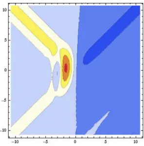
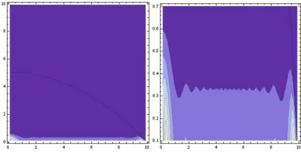
Figure 2.5: Plot of the charge density ρ for the wave function of an in-propagating wave packet propagating from left to right in the pair creation regime. The system parameters are again z0 = 10 and µ= 0.04. Since, in contrast to figure 2.4, this plot’s scale is linear the additional reflections at the kinks are not visible.

Despite the fact that one can investigate additional reflection effects effectively, the amplitude we considered in the last passage is not suitable to investigate the pair creation behaviour; it does not consider the charge of the particles and its spatial integral is not a conserved quantity. To get better insight into the pair creation one has to investigate the Klein-Gordon charge density (2.16). In figure 2.5 one can see the charge density for in-propagating particle states from the left in different regimes.

The enhanced out-propagating negatively charged wave packet and the additional positively charged wave packet propagating to the right are a manifestation of the pair creation. The quantitative calculation of the pair creation rate is the aim of the next chapter.

2.2 Spinor particles

The Dirac equation is

-iDµγ^µ− mc

!

.Ψ = 0 (2.23)

(21)

As we did for the solution space of the Klein-Gordon equation we use the charge, up to the factore, as an inner product.

(Ψ1,Ψ2)D =−i +

d³xΨ^†₁Ψ2. (2.24)

Again Dµ = ∂µ +i_!^qAµ and A0 is given by (2.3). Sauter already calculated the solutions of this equation in [19]. To get clearer insight into the solutions we use a slightly different and much simpler ansatz: we calculate the solutions of a quadratic spinor wave equation with a spin transport term and get the solutions of the dirac equation by using a projection operator (see ref. [9], [20] and [21]).

We define

Ψ =:-

iDµγ^µ+mc

! .

Z (2.25)

and get the quadratic equation

!

D^µDµ−i1 2

e

!cγ^µγ^νFµν+ m²c²

!²

"

Z = 0 (2.26)

where Fµν is the field strength tensor of the external electromagnetic field. Equation (2.26) dif- fers from the Klein-Gordon equation (2.1) for each spinor component only by the spin transport term −i^e₂γ^µγ^νFµν. For a general external electromagnetic field these equations can be decoupled by diagonalization of the spin transport term. To distinguish different spin states we consider the finite extended electric field corresponding to the potential (2.3) superimposed by a magnetic field inx3-direction. Thus we get

−i1

2γ^µγ^νFµν =



 Bσ₃ −iEσ₃

−iEσ3 Bσ3



 (2.27)



 1 0





(22)

The matrix (2.27) has four eigenvalues λρ,s = ρiE − sB where ρ, s ∈ {−1,+1}. λ_±1,+1 and λ_±1,−1 correspond to spin up and spin down states in x3-direction respectively. The corresponding eigenvectors are

Γ₋1,−1 = ^√¹₂





 1 0 1 0







Γ+1,−1 = ^√¹₂





 1 0

−1 0







Γ_−1,+1 = ^√¹

2





 0 1 0 1







Γ_+1,+1 = ^√¹

2





 0 1 0

−1





 .

(2.28)

Thus, with Zρ,s = φρ,sΓρ,s and equation (2.26), we get four independent second order differential equations

!

D^µD_µ+ e

!cλ_ρ,s+ m²c²

!²

"

φ_ρ,s= 0. (2.29)

We can solve each of these equations in the same way as we did for the Klein-Gordon equation in section 2.1.1. Since we only need the magnetic field for the identification of spin states we setB = 0.

In section II of diagramm 2.1 we then get an additional ρ-dependent term for the parameter n of the parabolic cylinder function. We define n(ρ) := iµ² − ¹₂ − ^ρ₂. For the identification of in- and out-propagating states we again use their asymptotic properties and the identification scheme of ref.

[14]. Thus we obtain solutions like in equation (7.5) and (7.6) wheren is replaced by n(ρ) and

c^L

R = 1

'2π0(±)(π0(±) +µ) and c^L

R = 1

'2π0(±)(π0(±)−µ)

for particle and antiparticle states respectively.

(23)

We get the corresponding solutions of equation (2.23) by using equation (2.25) in the form

Ψ˜ρ,s=-

iDµγ^µ+mc

! .

φρ,sΓρ,s. (2.30)

The rank of this projection is two and thus the 4× ∞-dimensional solution space of equation (2.26) is projected onto the 2× ∞-dimensional solution space of equation (2.23). For every pair of values for energy and transversal momentum we get four different solutions, i.e. two for each spin direction and we have to use an additional asymptotic condition to determine our solutions uniquely. In the absence of any background field, i.e. in Minkovski space, we can construct the different spin states by applying the irreducible standard representation of the Lorentz group on the four dimensional vector space of spinors generated by σ^µν = ¹₂[γ^µ, γ^ν] and the solutions of the equations [±γ⁰−1] Ψ = 0 given by

Ψ^(p)_−σ =N_p=0^(p)





 u_σ



 0 0









 Ψ^(a)_−σ =N_p=0^(a)









 0 0





uσ





 (2.31)

where^(p) denotes a particle and ^(a) an antiparticle, Np^(p,a) is a normalization constant and

u+1 =



 1 0



 u₋1 =



 0 1



 (2.32)

are the eigenvectors of the Pauli matrix σ3 to the eigenvalue σ = +1 andσ =−1 respectively in the standard representation.

We find

Ψ^(p)₋_σ =N_p^(p)



 (˜π0+µ)uσ

(.σ·p)u˜ _σ



 Ψ^(a)₋_σ =N_p^(a)



 (.σ·p)u˜ σ

(˜π₀ −µ)u_σ



 (2.33)

where.σ = (σ1, σ2, σ3) is the vector of Pauli matrices ¹.

(24)

As mentioned above for every pair of values for energy and transversal momentum the corresponding subspace of the solution space of the Dirac equation is two dimensional. Thus, in the asymptotic section I and III of the domain, the particle and antiparticle states can be written as linear combinations of the Minkovski space spinor solutions. For particle states we can write

Ψ˜^(p)s



 z ∈I z ∈III



= 5

σ







 (˜π₀(∓) +µ)u_σ (σ·p˜₋(∓))uσ



A^(p)_∓_,s,σe^−i˜^p(∓)z

+



 (˜π0(∓) +µ)uσ

(σ·p˜₊(∓))u_σ



B_∓^(p)_,s,σe^i˜^p(∓)z





(2.34)

and for antiparticle states

Ψ˜^(a)s



 z ∈I z ∈III



= 5

σ







 (σ·p˜₋(∓))uσ

(˜π0(∓)−µ)uσ



A^(a)_∓,s,σe⁻ⁱ^p(^˜^∓^)z

+



 (σ·p˜₊(∓))u_σ (˜π0(∓)−µ)uσ



B_∓^(a)_,s,σe^i˜^p(∓)z





(2.35)

where ˜p_±(∓) = (˜p₁,p˜₂,±p(˜∓)).

Now the missing asymptotic condition can be formulated as the statement that an in-propagating state is represented by a wave function with an in-propagating part with defined spin, that is in the asymptotic regime the in-propagating part of the wave function has to be equivalent to one of the Minkovski space solutions of the Dirac equation with defined spin and defined particle or antiparticle character. We handle the out-propagating states analogously. Using this asymptotic condition the coeffizientsAs,σ andBs,σcan be fixed and, for particle and antiparticle states, we obtain the following

(25)

expression:

Ψ˜^(p)_s = 1 2

6Ψ˜1,s+ ˜Ψ₋1,s

7 Ψ˜^(a)_s = 1 2

6Ψ˜1,s−Ψ˜₋1,s

7. (2.36)

Full expressions for some of these solutions are given exemplarily in the appendix 7.4. Finally with the inner product (2.24) and after some cumbersome calculations that are mainly equivalent to those for the solutions of the Klein-Gordon equation in Appendix I we get the following orthogonality relations:

(Ψ^(p,a)_in,out,(p(_±_),s),Ψ^(p,a)_in,out,(p_"₍_±_),s_"₎)D = 2π!δ(p(±)−p^$(±))(2π!)²δ⁽²⁾(p_⊥−p^$_⊥)δss^"

(Ψ^(p,a)in,out,p(−),Ψ^(p,a)_in,out,p"(+))D = 0.

(2.37)

(26)

Chapter 3 Field quantization

The next step on the way to quantum electrodynamics is to go from a one particle to an n-particle theory allowing particle creation and annihilation, with other word we must construct a quantum field theory from the one particle theory. We start with the case of scalar particles. The first task when constructing a quantum field theory is to specify the one particle Hilbert space and construct the Fock space from this. Our construction is closely orientated on the field theory construction outlined in ref. [24] and [25]. Since it is invariant under time evolution and, from a physical point of view, very natural we use the Klein Gordon inner product (2.18) as the inner product for our one particle Hilbert space. It must be mentioned, however, that the term “inner product” is misleading, since it is not positive definite. We must first split the solution space S of the Klein Gordon equation (2.1) to construct a positive definite inner product. The normalization in chapter 2 gives us the required splitting condition. We define Ain,out as the set of in- and out-propagating functions respectively which we constructed in chapter 2 and perform the split

A^±in,out:={f ∈ Ain,out : (f, f)KG

>

<0}. (3.1)

As outlined in chapter 2 this is equivalent to the decomposition into particle and antiparticle states.

The next step is to construct two separate inner product spaces fromA^±in,out. We define the linear

(27)

space

S˜in,out^± :={

f inite8

n

λ_nf_n :f_n ∈ A^±in,out, λ_n ∈C} (3.2)

and a scalar product on it by the definition

,f, g-±:=±(f, g)KG for f, g ∈S˜in,out^± . (3.3)

Since this is positive definite we get a pre-Hilbert, or inner product, space.

H˜^±in,out:=6

S˜in,out^± ,,·,·-±

7 (3.4)

Now we need a metric on ˜Sin,out^± to complete the pre-Hilbert space to a Hilbert space. One usually uses the metric induced by

g(f, g) :=,f −g, f−g-. (3.5)

Unfortunately our inner product is not finite for every element of ˜Sin,out^± . Since these unnormalizable states cannot exist in quantum mechnics we have to smear out the elements of ˜Sin,out^± with appropriate smearing functions to get physical states. Due to this physical argument we go on with our construction assuming that the elements of ˜Sin,out^± are normalizable¹.

By cauchy completion we get a complete spaceHin,out^± :=9

Sin,out^± ,,·,·-:

and by factorizing out the kernel of the product,·,·-we get a Hilbert space, that is a complete inner product space with positive definite inner product, with ˜Sin,out^± as a dense subset. H^±in,outis the one particle Hilbert that we require to define a Fock space. With the help of the symmetrization operatorsP_n⁺φn= _n!¹ 5

πφn(xπ1, ..., xπn) with φn ∈(H^±)^⊗ⁿ we define

FB^±:={αΩ :α ∈C} ⊕^∞n=1P_n⁺9

(H^±)^⊗n:

(3.6)

1It should be possible to give a mathematically clear construction by using the theory of generalized functions [26]

(28)

where Ω is the vacuum state. We callFB⁺the particle Fock space andFB⁻the antiparticle Fock space.

The next step on the way to a quantum field theory is to define creation and annihilation operators.

We define the creation operator c^†_in,out as a linear map from the one particle Hilbert space to the space of linear operators on the Hilbert space, i.e.

c^†_in,out : Hin,out → L(FB) f /→ c^†_in,out(f)

where c^†(f)Ω =f

with (c^†(f)Φ)n(x1, ..., xn) =√

nP_n⁺(f(x1)φn−1(x2, ..., xn)), n= 1,2, ... and

cin,out : Hin,out → L(FB) f /→ cin,out(f)

where c^†(f)Ω = 0

with (c(f)Φ)_n(x₁, ..., x_n) = √

n+ 1;

d³xf^∗(x)φ_n+1(x, x₁, ..., x_n), n= 1,2, ...

(3.7)

With these definitions we get, after some calculations [25], the commutation relations

[cin,out(f), c^†_in,out(g)] =,f, g-, [cin,out(f), cin,out(g)] = 0.

(3.8)

In [25] the author proves that every irreducible representation of the commutation relations (3.8) with vacuum Ω is unitary equivalent to the Fock representation constructed in (3.6). Thus by defining creation and annihilation operators for the particle and antiparticle Fock space and by defining the total Fock space FB :=FB⁺⊗ FB⁻ we get a well defined many particle theory. Finally we define the

(29)

field operator

Ψ(x) =; _d²_p_⊥

4π²!²

5

d∈{+,−}

;_∞

0 dp(d)

2π!

6ain(p(d), p_⊥)Φ^(p)_in,p(d)+b^†_in(p(d), p_⊥)Φ^(a)_in,p(d)7

=; _d²_p_⊥

4π²!² 5

d∈{+,−}

;_∞

0 dp(d)

2π!

6

aout(p(d), p_⊥)Φ^(p)_out,p(d)+b^†_out(p(d), p_⊥)Φ^(a)_out,p(d)7 (3.9)

where theain(p(−), p⊥) = a(Φ^(p)_in,p(d)) and theb^†_in(p(−), p⊥) =b^†(Φ^(a)_in,p(d)) are the particle annihilation and antiparticle creation operators respectively.

To argue that this is the correct form of the field operator and to get the unitary, dynamic time evolution operator we use the decomposed field operator to expand the Hamiltonian in terms of creation and annihilation operators. The Lagrangian density for the charged Klein-Gordon field is given by

L =!c )

(DµΨ)^∗D^µΨ− m²c²

!² Ψ^∗Ψ

*

. (3.10)

After some rearrangements we find

H =!c +

d³x )

∂0Ψ^∗∂0Ψ−e²A²₀Ψ^∗Ψ + m²c²

!² Ψ^∗Ψ + (DiΨ)^∗DiΨ

*

. (3.11)

Since we do not want to vary this Hamiltonian to get some equations of motion we are free to confine Ψ as a linear combination of solutions of the Klein-Gordon equation (2.1). By using the Klein-Gordon equation, partial integration and the definition of the Klein-Gordon inner product (2.18) we get for the Hamiltonian

H = i!

2(( ˙Ψ,Ψ)KG−(Ψ,Ψ)˙ KG). (3.12)