Analysis of CRESST Dark Matter Search Data

(1)

PHYSIK-DEPARTMENT

Analysis of CRESST Dark Matter Search Data

Diploma Thesis by Florian Reindl

7th of December, 2011

(2)

The CRESST (Cryogenic Rare Event Search with Superconducting Thermometers) experiment aims to detect WIMPs (Weakly Interacting Massive Particles). WIMPs are currently one of the most promising candidates for the explanation of Dark Matter. A short introduction on evidence and candidates for the Dark Matter is given in chapter 1.

CRESST uses scintillating crystals with superconducting thermometers, operated at mK temperatures, to observe WIMP scatterings off nuclei. More details about the CRESST experiment, including a discussion of backgrounds, are presented in chapter 2.

In this work a complete data analysis of the latest run (run 32) was performed. The available analysis was improved in several aspects. Chapter 3 describes necessary data preparations. Each particle pulse is fitted with a so-called standard pulse. The amplitude of the pulse, as determined by this fit, is then used to determine the energy of the particle interaction (also discussed in 3). Therefore, it has to be ensured that all events which do not guarantee a correct determination of the amplitude and thereby the energy are withdrawn. In this work most emphasis was put on the development of a cut on the RMS.

The RMS is a measure of the deviation from a particle pulse and the standard pulse and therefore an universal parameter to detect events of different pulse shape not assuring for a correct energy determination. However, the RMS is energy and time dependent and the correlation of the two dependencies makes a simple cut on the RMS unfeasible.

The time dependence arises from changing detector noise. Thus, a new method was developed which is capable to track changes in the detector noise (see chapter 4). In chapter 5 the new energy dependent cut on the RMS is presented which is, in cooperation with the noise tracking, automatically adjusted to different noise levels in different time periods.

The next section (5.4) deals with muon-induced events detected by the muon veto surrounding the experiment. The existing cut was successfully modified in order to improve its time resolution.

The ultimate goal of this work was to provide a second and independent analysis of

the data taken in the latest run. The latter was the first extensive physics run of the

CRESST experiment and in a recent publication of the CRESST collaboration ([1]) an

excess over the expected background contributions, which is compatible with a light

WIMP scenario, was observed with a statistical significance of more than 4σ. In order

to be able to compare the analysis of this work with the one in [1] the processed raw

data of this work was used to perform a maximum likelihood analysis. Chapter 7 offers

the corresponding results.

(6)

1. Dark Matter

The famous paper “Die Rotverschiebung von extragalaktischen Nebeln” [2], which was published by F. Zwicky almost 80 years ago in 1933, gave birth to the term Dark Mat- ter. F. Zwicky found that the luminous mass of the COMA cluster makes up a minor contribution in the total mass density of the cluster only. He therefore assumed that there has to be additional non-luminous matter, the Dark Matter. This observation was the first indication for the existence of the Dark Matter. Since then a lot of additional observations enriched the picture of the Dark Matter. Today it is known, that ordinary baryonic matter contributes only with 4.56% (data from [3]) to the total energy density of the universe. The contribution of non-baryonic matter is 22.7%. The largest con- tribution of 72.8% is attributed to the so-called Dark Energy. However understanding the nature of the Dark Energy is up to now beyond the reach of physicists. In contrast, various theories, such as additional elementary particles, exist in order to explain the Dark Matter. The search for Dark Matter is the aim of the CRESST experiment.

This introduction will briefly describe convincing evidence for Dark Matter found on various astronomical scales. Possible Dark Matter candidates are discussed afterwards.

1.1. Evidence for Dark Matter

This section will briefly introduce the main observations which point to the existence of the Dark Matter and, furthermore, which information on the nature of the Dark Matter can be derived from the various observations.

1.1.1. Cosmic Microwave Background

The Cosmic Microwave Background (CMB) allows a precise measurement of many cos- mological parameters. It opens up the possibility to look back to times about 380.000 years after the Big Bang. In even earlier times the temperature of the universe was that high, that combination and recombination of a proton and a electron to hydrogen (p + e

⁻

H) were in equilibrium. Therefore the number of free electrons and protons was large and the interaction rate of radiation with electrons and protons, via Thomson scattering, was high.

With the expansion and cooling of the universe to temperatures of 0.3 eV (or 3000 K)

the disintegration of hydrogen (p + e

⁻

← H) was not possible any more and the re-

combination (→) caused a disappearance of nearly all free charged particles, which lead

to hardly any interaction between radiation and matter any more. In other words: the

photons decoupled and the universe became transparent. Quite some measurements of

(7)

1. Dark Matter

the CMB were made and it was found that its spectrum is nearly a perfect black body spectrum which is expected, because of the thermal equilibrium before the decoupling.

The temperature of the CMB today is 2.725 K ([3]).

Figure 1.1.: Image of the cosmic microwave background. The dipole term, introduced by the motion of the earth, is already subtracted. It shows that the matter density at the time of recombination was nearly perfectly homogeneous, but still some fluctuations at the level of 10

⁻⁵

were found, which make calculations on, for instance, the Dark Matter density possible. (Image taken from [4].)

Furthermore the experiments, in particular the satellite experiments (COBE, WMAP and Planck), studied the homogeneity of the CMB. After subtracting the dipole term, which is caused by the motion of the earth, only deviations at the level of 10

⁻⁵

from a perfect isotropy were found (see figure 1.1). These small inhomogeneities are caused by gravitational redshifts and thus reveal tiny fluctuations of the matter density at the time of the recombination. By investigating the angular scale on which they occur it is possible to determine the density of Dark Matter (non-baryonic matter) to be Ω

_DM

= 0.227.

1.1.2. Structure Formation

Tiny fluctuation of the matter density in times shortly (on cosmological scales) after the Big Bang, as mentioned above, lead to the large-scale structure of the visible matter.

This large-scale structure was, for instance, studied by the Sloan Digital Sky Survey

collaboration ([5]). The Millenium Simulations ([6]) try to model these tiny fluctuations

and to simulate their evolution with time. By comparing the results of the simulations

with today’s observations it turned out that the current structure of the universe can

not be explained without additional non-baryonic matter. Moreover the amount of non-

baryonic matter, which has to be included in the simulation, is in very good agreement

with for example the results from CMB measurements. In conclusion one can say that the

consistent picture between simulation and observation, which can only be achieved with

(8)

1. Dark Matter

a non-baryonic matter component, further substantiates the evidence for the existence of Dark Matter.

1.1.3. COMA and Bullet Cluster

The next step to smaller cosmological scales is to look at structures of many galaxies, the so-called clusters. Two different observations on the scale of galaxy clusters are presented here, with the first one being the oldest hint for Dark Matter and the second one being the most recent evidence for it.

COMA Cluster

The observation of F. Zwicky in 1933, which brought up the search for Dark Matter, today is supported by several measurements of different clusters with compatible results.

The mass of a galaxy cluster can be determined in different ways. The first is to connect the average velocity (average kinematic energy) of the galaxies in the cluster, by using the virial theorem, to the gravitational potential and thereby to the mass. The second way is based on the known correlation between the mass of an object and its luminosity. F. Zwicky used both possibilities and found a discrepancy between the total mass and the luminous mass of the COMA cluster. The missing non-luminous mass he then called Dark Matter.

Bullet Cluster

The observation of the mass distribution in the so-called Bullet cluster [7] in 2004 is widely seen as a proof for the existence of Dark Matter, because it is a “direct” obser- vation of the Dark Matter and it is not compatible with the so-called MOND-theories, which will be briefly introduced in subsection 1.1.4, as a stand-alone explanation. The Bullet cluster actually is a collision between two galaxy clusters, with one of the clusters being much smaller (the bullet) than the other one.

The stars of both clusters nearly pass each other without being effected in the collision

of the clusters. In contrast the components of the fluid-like plasmas of both galaxies,

which were traveling along with the stars, interact electromagnetically with each other

causing the plasmas to slow down. This is why a collision of two clusters spatially

separates plasma and stars. It is known that stars are in general only a minor component

to the total mass of a cluster. The dominant component is the fluid-like plasma. Such a

hot plasma is emitting X-rays and by measuring them it is possible to localize it. Via the

effect of gravitational lensing it is possible to deduce the gravitational potential out of

optical images. Both techniques were used to get the pictures in figure 1.2. On the left

side an optical image of the Bullet cluster is shown. The contour lines, which are plotted

in both images, indicate the gravitational potential. One would expect to observe the

highest mass density at the position of the plasma. However, looking at the right X-ray

image of the bullet cluster it can be seen, that the position of the plasma clearly differs

from the two centers of masses. It is obvious that additional matter could explain this

(9)

1. Dark Matter

Figure 1.2.: Shown are two images of the so-called Bullet cluster, with the left one being an optical image and the right one being an image generated by the measurement X- rays emitted by the plasma. The contour lines in both images illustrate the gravitational potential (measured by gravitational lensing) and it can be seen that the two centers of masses do not coincide with the position of the plasma. (Images taken from [8].) separation perfectly. Since the centers of masses are roughly at the positions of the stars, a weak interaction of this additional component is required, because otherwise it would have been slowed down in the collision, just like the plasma. In conclusion it is to state that the observation of the Bullet cluster directly proves the existence of a non-luminous and if at all weakly interacting matter component.

1.1.4. Rotation Curves

Rotation curves are functions, which express the velocity of a star as a function of the distance between the star and the corresponding galactic center. For many galaxies, in particular for spiral galaxies, the distribution of the stars can be approximated by a flat and rotating disk. The total mass of a galaxy can be measured by the known correlation between luminosity and mass. Once the total mass of a galaxy is determined, the velocity of stars can be calculated using the following equation:

1 2 mv(r)

²

= G mM (r)

r ⇒ v(r) =

r GM (r)

r (1.1)

M(r) is the mass of the galaxy dependent on the distance to the galactic center r. m and v are mass and velocity of the star and G is the gravitational constant.

However since practically the whole mass of the galaxy is concentrated within the radius of the disk, M(r) gets constant for radii larger than the radius of the galactic disk and the velocities of stars outside the disk should be decreasing (v(r) ∼

^√¹_r

).

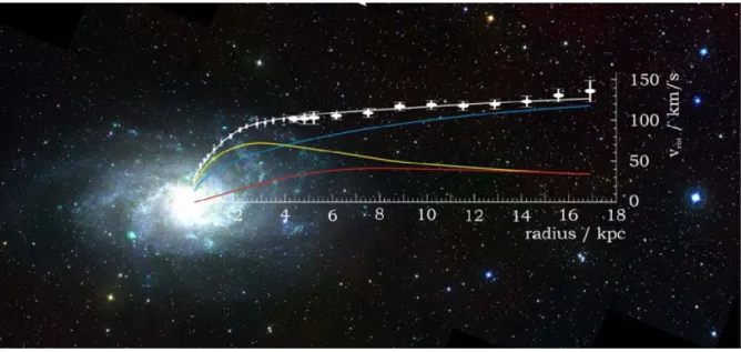
The example of the galaxy M33 in figure 1.3 shows, that no decreasing, but a roughly

constant (v(r) ∼ const) behavior of the velocities for large radii can be observed. The

discrepancy between expectation and observation can easily be solved by postulating a

spherical Dark Matter halo. The halo’s matter density has then to be ρ(r) ∼

¹_r

and its

(10)

1. Dark Matter

Figure 1.3.: In this overlay the measured rotation curves (white crosses) and a image of the galaxy M33 can bee seen. The colored lines show the contributions to the best fit (white line) to the measured data. The yellow line arises from the contribution of the visible mass and the red line from a contribution of gas. Only by adding a Dark Matter contribution (blue line) the observation can be explained. (Picture taken from [9]) radius has to be several times the radius of the visible galactic disc. Since there is no indication for the Milky Way not to be a typical spiral galaxy, the Dark Matter halo should also be present in “our” galaxy. Thus the expected velocities of potential Dark Matter particles and the expected density profile of Dark Matter in the Milky Way itself can be calculated (for a detailed calculation see for example [10]).

Another explanation for the rotation curves are the so-called MOND-theories (MOd- ified Newton Dynamics). These theories are based on the assumption, that Newton’s second axiom might be different for small accelerations (stars outside the galactic disk) and large accelerations (every-day experience). Such a modification could in fact de- liver suitable rotation curves. However, apart from the lack of a proper motivation to consider such a modification, MOND-theories are not compatible with the structure formation and, in particular, with the observation of the Bullet cluster (see subsection 1.1.3). Therefore the MOND-theories today are strongly disfavored with respect to Dark Matter explanations.

1.2. Candidates for Dark Matter

1.2.1. Baryonic Dark Matter - MACHOs

As a first approach to explain Dark Matter it is quite obvious to study whether the

existence of Dark Matter can be explained by “ordinary” baryonic matter. Massive

(11)

1. Dark Matter

(Astrophysical) Compact Halo Objects are such baryonic candidates. They can be for example brown dwarfs, neutron stars or black holes. MACHOs can be detected via micro lensing and indeed some hundred were found (for example by the MACHO project: [11]).

However in [12] it is shown, that the number of found MACHOs is by far not sufficient to explain Dark Matter completely. Furthermore some evidence for Dark Matter, especially the CMB and the structure formation, require the largest fraction of the Dark Matter to be non-baryonic. This section will therefore continue with the presentation of non- baryonic Dark Matter candidates.

1.2.2. Non-Baryonic Dark Matter

Elementary Particles

Elementary particles are very promising Dark Matter candidates if they fulfill the fol- lowing requirements.

• The interaction rate of an elementary particle has to be very low, because otherwise it would most probably have been observed already. Especially it has to be elec- trical neutral, since a possible emission or absorption of electromagnetic radiation would hardly have remained undetected. Furthermore, in order not to participate in the strong interaction, it has to be color-neutral. Of course it is required for the particle to have a mass, because, as presented before, all evidence for Dark Matter are based on the observation of its gravitational interaction. The ability of such a particle to couple weakly to ordinary matter is allowed, but, although assumed by the experiments, not necessary.

• The attributes of a elementary particle as a Dark Matter candidate have to be in accordance with the model of the nucleosynthesis in the Bing Bang. Furthermore it has to be consistent with simulations of the formation of stars.

• The present structure of the universe can not be explained with Hot Dark Matter (HDM) alone. Hot means that the particles were relativistic at the time considered.

The existence of a large amount of relativistic particles, at the time of structure formation, would cause matter density fluctuations to be equalized faster than the time which is needed to form clumps of a certain size. Since the current structure of the universe is a result of these clumps evolving over time, elementary particles explaining the Dark Matter had to be non-relativistic at the time of structure formation. Non-relativistic elementary “Dark Matter particles” are referred as Cold Dark Matter.

• An elementary particle obviously has to exist today to explain the current obser-

vations. Furthermore it had to be present in the early universe in order to be

compatible with the CMB measurements and the simulations on the large-scale

structure formation. These aspects can be fulfilled in two possible ways. The first

possibility is that the particle is either stable, or its live time is at least in the order

(12)

1. Dark Matter

of the age of the universe. The second possibility is the existence of a production mechanism, which is able to compensate the reduction of the particle’s density due to its decay. Both cases, in particular the stable particle case, are not compatible with a destruction mechanism which is or was significantly reducing the particle’s density.

• Obviously the particle must not have been excluded by experiments. Apart from dedicated Dark Matter search experiments also, for example, high energy collider measurements are able to find signatures of possible Dark Matter candidates.

Neutrinos

Since quite some time it is known that neutrinos are not massless. Although up to now no precise values for the exact absolute neutrino masses could be measured, it is possible to give an upper limit for the sum of the masses of all three neutrino flavors (see [13]). Since this sum of masses is very low, neutrinos are ruled out as a stand-alone Dark Matter candidate. Furthermore neutrinos belong to the group of HDM and not to the CDM, which is needed to explain the structure of the universe. In conclusion one can say that the present knowledge of neutrinos indicates, that they provide only a negligible contribution to Dark Matter.

Axions

An axion is a hypothetical particle. It was named after a cleaning agent because its existence would wipe out the strong CP problem. The CP-symmetry is broken in the weak interaction and although the QCD allows for a non-zero CP-breaking phase, up to now all experiments measured this phase to be zero within uncertainties. High precision measurements on the magnetic dipole moment of the neutron are currently ongoing, because a CP-breaking of the strong interaction would result in a non-zero value for it.

Just like a π

⁰

meson the decay channel of an axion would be into two photons a → γγ.

Although the coupling of axions on photons would be rather small and therefore their life times would be quite high, axions produced in the Big Bang would already have been decayed. However via the Primakoff-effect axions could have been produced in reactions after the Big Bang with a high-energetic γ and a photon of the Coulomb field of a atomic nucleus. This axion production mechanism could take place in stars. Therefore, the axions would be a promising candidate for Dark Matter.

An experimental hint for axions would be the observation of an axion line in the elec- tromagnetic spectrum of the sky, because two monochromatic γ’s would be produced in an a → γγ decay. Furthermore for example the CAST experiment, located at the CERN laboratories in Geneva, is aiming to directly detect axions by reversing the Primakoff- effect, which means to convert an incoming axion with the aid of a strong transversal magnetic field

¹

into a mono-energetic photon, which can then be detected.

1

The magnetic field is generated by a common LHC magnet.

(13)

1. Dark Matter

WIMPs

Weakly Interacting Massive Particles are the most promising candidate to explain the Dark Matter with an elementary particle under the assumption, that they fulfill the requirements discussed above. In particular the mass (m

_χ

) of such a WIMP (χ) has to be large enough to be considered non-relativistic at the time of the structure formation and the WIMPs have to be stable (at least at time scales in the order of the age of the universe). In the early hot universe, when k

_B

T >> m

_χ

the WIMPs would have been in equilibrium with arbitrary other particles:

χ χ ¯ l ¯ l, χ χ ¯ q¯ q · · · (1.2) Equilibrium means that the rates of production and annihilation, which depend on the number density n

_χ

, are equal.

However with the expansion of the universe the WIMP density would have decreased and the WIMPs would have been able to leave the equilibrium (freeze-out). If no other destructive processes, decreasing the WIMP density exists, the abundance of WIMPs would have stayed constant after the freeze-out. The abundance today then would de- pend on the cross-section < σ

_A

v > of the annihilation process in equation 1.2. According to [13] their relic density would then be given as follows:

Ω

χ

h

²

' 0.1pb · c

< σ

_A

v > (1.3)

Assuming that nearly all Dark Matter exists in the form of WIMPs (Ω

DM

≈ Ω

χ

) the averaged (over temperature) cross-section can be calculated using the WMAP ([3]) value for the entire Dark Matter density Ω

_χ

h

²

= 0.1123:

< σ

_A

v >≈ O(10

⁻⁵

pb km/s) (1.4) In conclusion one can say that the existence of a WIMP, with the attributes mentioned above, provides an excellent explanation for the physical observations of the Dark Mat- ter.

Furthermore many theories provide possible WIMP candidates, with the supersym- metric extension (SUSY ) of the standard model being the most prominent one. In SUSY theories the standard model is extended by adding a supersymmetric partner to each standard model particle, whereas the spin of particle and supersymmetric partner is different by 1/2. One partner is then a fermion and the other one a boson. In most SUSY models a conserved quantity, the R-parity, is defined the following way:

R := (−1)

^3b+l+2s

(1.5)

The exponents are the baryon number b, the lepton number l and the spin s. Every

standard model particle then has a R-parity of R=1, whereas supersymmetric particles

have R=-1. This yields the Lightest Supersymmetric Particle (LSP) to be an obvious

WIMP candidate since, if the R-parity is conserved, the LSP can not decay into lighter

standard model particles. Many different SUSY models exist and many supersymmetric

particles are in discussion as possible LSPs, out of which the neutralino is the most

favored one.

(14)

1. Dark Matter

Direct and Indirect WIMP Search

As discussed before, WIMPs are the most favored candidates for Dark Matter. Fur- thermore, the chances to detect a possible WIMP by experiments are considered to be quite good. Thus, most Dark Matter experiments search for WIMPs in one of the two possible ways:

• One can search indirectly for WIMPs by detecting secondary particles, which could be produced by WIMP decays or annihilation. Currently several experiments are either already running or are still in preparation. Special emphasis is put on the detection of secondary γ-rays [14].

• The other possibility is to directly search for WIMPs by detecting interactions

between WIMPs and ordinary matter. The CRESST experiment belongs to the

class of direct Dark Matter searches and aims to detect WIMPs via their elastic

scattering off nuclei. The next chapter contains a more detailed description of the

CRESST experiment.

(15)

2. The CRESST Experiment

The CRESST (Cryogenic Rare Event Search with Superconducting Thermometers) ex- periment is directly searching for Dark Matter in the form of WIMPs. The basic idea behind this experiment is to detect the recoil of a nucleus induced by elastic scattering of a WIMP in a target.

Since the expected detection rate of WIMPs is very low ( . 0.1 kg

⁻¹

d

⁻¹

) all experi- ments directly searching for WIMPs have to aim for a reduction of backgrounds as far as possible.

One has to distinguish between passive and active background reduction. If a source of background is known and it is possible to clearly identify events from such a source, then an active background discrimination can be done. The CRESST detector modules offer this possibility, which is described in section 2.3. Passive background reduction on the other hand means to reduce the possible sources of backgrounds by shielding the experiment and by using radio pure materials. This chapter will begin with an overview over possible background sources and their consequences for the design of the experiment. Afterwards a description of the working principle of the detectors will be given.

2.1. Experimental Setup: Cryostat and Shielding

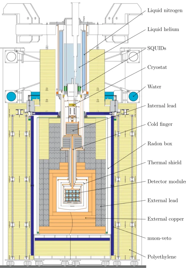
Figure 2.1 gives a schematic overview of the CRESST setup. The detector modules, which are located in the center of the experiment are connected to a

³

He/

⁴

He dilution refrigerators (cryostat) on top with a so-called “cold finger”. Cooling the detectors is necessary for their operation which will be described in section 2.3. Several layers of shielding surround the detectors, beginning with copper, followed by lead and polyethy- lene. The inner parts of the experiment are enclosed by a gas-tight box, the so-called Radon-box. Its purpose will be discussed along with the radon background. The whole experiment is surrounded by a muon veto. The SQUIDs used to read data from the detectors are located in the upper part of the cryostat.

2.2. Backgrounds

2.2.1. Muons

Cosmic muons make a large contribution to possible background sources. These muons

are a secondary product of cosmic rays interacting with the earth’s atmosphere. To

shield the experiment against them the setup is located in the Laboratori Nazionali del

(16)

2. The CRESST Experiment

Liquid nitrogen

Liquid helium

SQUIDs

Cryostat

Water

Internal lead

Cold finger

Radon box

Thermal shield

Detector modules

External lead

External copper

muon-veto

Polyethylene

Figure 2.1.: Schematic drawing of the CRESST experimental setup.

(17)

2. The CRESST Experiment

Gran Sasso (LNGS), an underground laboratory in the Abruzzi near Rome. 1400m of rock provide the amount of shielding which makes experiments like CRESST possible.

Since this natural shielding is by far not able to suppress cosmic muons completely the experiment is surrounded by the muon veto in order to tag particle interactions in coincidence with muons penetrating the experiment. This muon veto is composed of 20 plastic scintillation panels, each equipped with its own photo multiplier. Looking at figure 2.1 reveals that the muon veto has a hole in the top, which is necessary for the cryostat. Taking this hole and the finite efficiency of the muon veto into account, muons may still provide a background contribution.

Furthermore muons can also contribute indirectly to the background by producing neutrons outside the muon veto, for instance in the surrounding rock. Such neutrons may then penetrate the experiment with the muon not hitting the muon veto and therefore staying undetected.

2.2.2. Radon

The main radon exposure is caused by the radioactive isotope

²²²

Rn, which is part of the radium (uranium) decay chain starting with

²³⁸

U.

²²²

Rn decays via an α-decay to

218

Po. The radon gas leaving the surrounding rock is prevented from penetrating the inner shielding with the so-called radon box. The radon box is a gas tight box constantly flushed with radio pure nitrogen and kept under slight overpressure.

To avoid exposure of the detectors and the inner material to contaminated air (e.g.

during installation) is very important, because radon can be adsorbed on the surfaces.

2.2.3. Neutrons

A precise knowledge about the possible neutron background is necessary, because neu- tron events cannot always be distinguished from possible WIMP scatterings. The total neutron flux in the LNGS laboratory is dominated by neutrons from (α,n)-reactions on light elements and neutrons from spontaneous fission of heavy nuclei (mainly of

²³⁸

U ).

Although the rate of neutrons generated by interactions of cosmic muons is suppressed by several orders of magnitude, compared to earth’s surface, they still make an addi- tional contribution. Different measurements with quite different results of the neutron flux at LNGS were made. Two main issues for these measurements have to be consid- ered. First of all the low neutron rate makes an accurate measurement very hard and furthermore, the neutron flux seems to be quite different at different position in the LNGS underground laboratory. Taking both arguments into account, the discrepancies between the measurements are not surprising.

In [15] the results of a Monte Carlo simulation show a good agreement with the neutron flux measured in [16]. A rough estimate of the total neutron flux derived from this measurement gives a value of ∼ 60 − 140 neutrons per square meter and hour.

Fifty centimeters of polyethylene (PE) surrounding the experiment (see figure 2.1)

moderate neutrons down to energies less than eV. Such energies are below the trigger

thresholds of the detectors. Water was used instead of PE, where the installation of the

(18)

2. The CRESST Experiment

latter was not possible. PE is well suited to moderate neutrons due to its high content of hydrogen atoms. Since hydrogen atoms are roughly of the same mass as neutrons, a high amount of energy is transfered in scatterings.

With the PE being outside the lead and the copper shielding (see figure 2.1), neutrons produced by reactions of muons in the lead or the copper shielding can reach the detectors without being moderated. For the next run an additional PE layer inside the lead-copper shielding is planned to be added.

2.2.4. γ’s and Electrons

Since cosmic radiation is strongly reduced in an underground laboratory, γ’s (and elec- trons) from the natural decay chains of

²³⁸

U and

²³²

Th as well as from the isotope

⁴⁰

K are by far the dominant background. According to [17] the integral gamma flux at LNGS is roughly ∼ 1cm

⁻²

s

⁻¹

.

To shield this background a 20 cm thick layer of lead (24 t of weight) surrounds a 14 cm thick layer of copper (10t). Lead has a high atomic number and a high density.

These characteristics make it a very good shielding against γ’s. The disadvantage of lead is its intrinsic contamination with mainly

²¹⁰

Pb, which is part of the

²³⁸

U decay chain. Following this decay chain it can be seen that all types of radiation (α-, β- and γ- radiation) are emitted until the end of the chain is reached with the stable isotope

²⁰⁶

Pb.

Whereas the α- and β-radiation is not able to penetrate the cold box, the γ-radiation is seen as background in the experiment.

Copper, on the other hand, can be produced with a high radio purity and is therefore used as a shielding to suppress background from the lead shielding. Copper is for example also used for the holders of the detectors.

2.3. Detectors

CRESST can use different scintillating crystals as target material. In run 32 only CaWO

₄

crystals were used for the Dark Matter analysis (some ZnWO

₄

crystals were installed for test purposes). Two such crystals can be seen in figure 2.2. The cylindrical crystals are 40 mm in height and diameter and weigh about 300 g.

2.3.1. Target Material

The cross-section for coherent WIMP scattering off nuclei is assumed to be proportional

to A

²

, with A being the atomic mass of the target nuclei. Therefore, one would expect

to observe most WIMP scatterings off the heavy tungsten nuclei. However, this is not

the case for light WIMPs, because of the finite energy threshold of the detectors. For

kinematic reasons such a low-mass WIMP is not able to transfer a detectable amount

of energy on the tungsten nuclei. On the other hand, recoils of the light calcium and

oxygen nuclei can still be above the energy threshold of the detectors. In figure 2.4

the expected scattering rate of the three different nuclei is plotted as a function of the

(19)

2. The CRESST Experiment

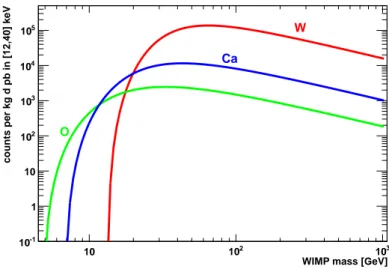
WIMP mass. Further assumptions are a cross-section of 1 pb and a detector, which is sensitive from 12 keV up to 40 keV. This range is typical of CRESST detectors. In this figure it can be seen that (starting from low WIMP masses) at first oxygen, then calcium and finally tungsten recoils contribute to the total rate. For WIMP masses higher than

∼ 30 GeV tungsten recoils dominate the scattering rate, whereas for WIMP masses less than ∼ 20 GeV tungsten recoils are completely below threshold. Going down from 20 GeV to even lower WIMP masses calcium recoils contribute down to WIMP masses of ∼ 5 GeV. Below a WIMP mass of ∼ 2 GeV not even oxygen recoils can be detected any more with the assumed detector sensitivity.

Figure 2.2.: Two scintillating CRESST CaWO

₄

crystals illuminated with UV light.

Figure 2.3.: A photograph of a so-called composite crystal. For composite crys- tals the thermometer (tungsten film) is not evaporated directly onto the crystal, but onto a small carrier crystal which is then glued to the big target crystal.

2.3.2. Measurement of Phonons and Light

Figure 2.5 gives a schematic of a CRESST detector module (a photograph can be seen in

figure 2.6). A detector module contains two (three) cryogenic calorimeters. One phonon

and one (two) light detector(s). As described in the section above, the target material

is a scintillating CaWO

₄

crystal. A crystal from this material is the central element of

each phonon detector. Any particle interaction in the crystal will excite phonons. As a

thermometer for measuring these phonons a transition edge sensor (TES) is used. The

principle of a TES will be described in more detail in the next subsection (2.3.3). The

crystal together with its thermometer is called the phonon detector. The thermometer

is a tungsten film which is either evaporated directly onto the crystal (conventional)

or evaporated onto a small carrier crystal (see figure 2.3), which is then glued to the

target crystal (composite). Discussion about the advantages and disadvantages of both

techniques can be found in [18]. A thermal coupling is needed to relax the detectors back

to working temperature after the heating up due to a particle interaction.

(20)

2. The CRESST Experiment

WIMP mass [GeV]

10 10² 10³

counts per kg d pb in [12,40] keV

10-1

1 10 102

103

104

105 W

Ca

O

Figure 2.4.: Three different nuclei are present in the CaWO

4

target crystal. Plotted is their contribution to the total interaction rate of WIMPs as a function of the WIMP mass. The presented calculation is based on a cross-section of 1 pb and assumes coherent

∼ A

²

scattering. The lower energy threshold of the virtual detector was set to 12 keV and the upper one to 40 keV. (Figure taken from [1])

TES

target crystal

TES reflective and scintillating housing light

detector

phonon detector

light absorber thermal coupling

thermal coupling

Figure 2.5.: Schematic drawing of a CRESST detector module. The phonon detector consists of the target crystal (in- stalled in run 32: CaWO

4

and ZnWO

4

) and a transition edge sensor (TES). The light detector is used to measure the scin- tillation light leaving the target crystal. It carries another TES. A detector module is surrounded by a light reflecting foil which also scintillates.

Figure 2.6.: A picture of an opened detec-

tor module in the configuration which was

used during run 32. The light detector is

on the left side and the phonon detector on

the right side. On top of the crystal one

can see the transition edge sensor, which

is connected via bond wires. The detec-

tors are connected with their holders (cop-

per) with uncovered clamps. Furthermore

the reflecting foil surrounding the detector

module can be seen.

(21)

2. The CRESST Experiment

The signal of the phonon detector gives a measure of the total deposited energy.

However, a small fraction (O(1%)) of the transfered energy will not be converted to phonons, but to scintillation light. The amount of light depends on the type of particle interaction. The scintillation light can (at least part of it) leave the crystal. To measure it, a light absorber is installed above the crystal. This absorber is also equipped with an evaporated TES. The light absorber together with the corresponding thermometer is called a light detector. As absorbers, mostly cylindrical so-called silicon-on-sapphire wafers with 40 mm of diameter and 0.46 mm of height are used. The silicon layer itself is 1 µm thick. Some light detectors, however, consist of pure silicon. The light detector is thermally coupled to the cryostat, just like the phonon detector.

The whole module is surrounded by a scintillating and reflecting foil to collect as much light as possible in the light absorber. For test purposes one detector module, which was installed in run 32, had two light detectors facing the two circular surfaces of the crystal.

2.3.3. Cryogenic Calorimeter with Transition Edge Sensor

Figure 2.7.: Shown is the resistance of a tungsten film over the temperature (taken from [10]).

An energy deposition by a particle interaction in a calorimeter leads to a rise of the temperature in the latter. The dependence of temperature and energy is given by the following equation:

∆T = ∆E

C (2.1)

(22)

2. The CRESST Experiment

C is the heat capacity, which for a dielectric material at low temperatures, takes the form:

C ∝ ( T Θ

D

)

³

(2.2)

with Θ

_D

being the Debye temperature (see e.g. [19] p. 212).

Looking at equation 2.1 reveals that a low heat capacity is needed in order to maximize the temperature rise ∆T . Equation 2.2 shows that low temperatures are necessary for a small heat capacity. However, even at very low temperatures (O(10 mK)), the temperature rise is only in the order of µK. To read out these small temperature changes, CRESST detectors use tungsten transition edge sensors operated in the normal to superconducting transition at temperatures in the order of 10 mK. Figure 2.7 shows such a transition. If the film is in the transition, then a small change in temperature

∆T will result in a detectable large change in resistance ∆R. With this technique even tiny energy depositions (below a few keV) in the crystal can be measured.

Every tungsten film used as a thermometer has a heater. This heater is needed to keep the temperature of the detector at a constant operating point. How this is done will be described in the next subsection (2.3.4). Fur sufficient small energy depositions the resistance (∆R) changes linearly with the temperature (∆T ) around the operating point. But even for events with too high energies for a linear approximation of the resistance-energy dependence a pulse shape analysis can be made, which will be the topic of the truncated standard pulse fit in section 3.3.

2.3.4. Detector Operation and Data Acquisition

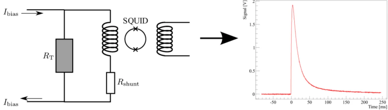
Figure 2.8.: A simple overview over the parallel circuit of the TES (R

_T

) with R

_shunt

and the input coil of the SQUID. Using this circuit the initial thermal pulse is converted into an electrical pulse (right side). (Taken from [10].)

To read the current electric resistance of the TES (R

T

) the sensor is connected in a parallel circuit with a resistor (R

_shunt

) and a coil used for a inductive coupling to a SQUID

¹

. A circuit diagram can be seen in figure 2.8. A current source injects a constant

1

A SQUID (for

Superconducting QUantum Interference Device) is a device to measure very weak

magnetic fields.

(23)

2. The CRESST Experiment

current (I

_bias

∼ O(µA)). If the resistance of the TES changes, the current partition between the film and R

_shunt

will change. This change will then be registered by the SQUID. Using this procedure the warming of the TES will be transfered into a electrical signal which then can be further processed.

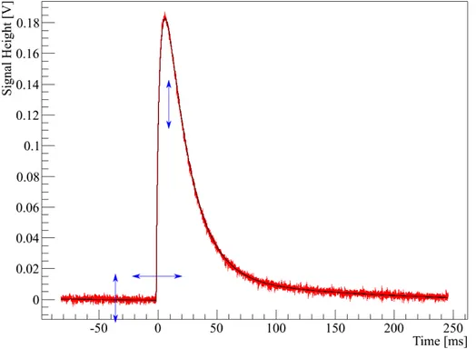
The SQUIDs are connected to a transient digitizer which continuously samples the signal. Eight of these digitizers are enclosed in one digitizer module. For each detector a trigger threshold is defined and whenever a signal above the threshold is recognized a record of the detector and all other detectors of the same detector module are saved to disk. A complete record consists of 8192 samples with 16 bit each. The sampling rate is 25 kHz and thus a complete record extends over a time of 327.68 ms. In order to obtain information on the baseline of each pulse the signal in a certain time period before the trigger is stored. This pre-trigger region has a length of 81.92 ms which is a quarter of the whole record. The time period from the trigger to the end of the record is called the post-trigger region. Only in the first half of this post-trigger region the other detectors on the same digitizer module (up to seven) are allowed to trigger. The triggers are not being activated right away after the end of the record for two reasons. Firstly, a certain time is needed to read out and save all digitizer channels which triggered. Secondly, in order to satisfyingly sample the baseline, it is necessary to deny a instantaneous reactivation of the trigger after the read out. While the second aspect would only require to wait for the length of the pre-trigger region it was decided to double the waiting time to twice the length of the pre-trigger region, because otherwise the number of records just containing the decaying tail of a prior (large) pulse would be very high. On the other hand, for test pulses, which will be discussed in the following, the enforced waiting time is equal to the length of just one pre-trigger region.

Control and Test Pulses

As discussed before, each detector is equipped with a heater. Firstly, a constant current is applied to the heater with the aim to keep the detector at the desired temperature.

Secondly, at certain times control and test pulses are injected to the heater.

Control pulses are large pulses driving the TES completely out of its transition. With their help the current position of the detector in the transition can be determined and the constant heater current can be regulated such that the detector is stabilized in its previously defined operating point (see figure 2.7).

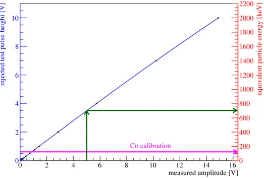
Test pulses are tiny pulses (injected with different pulse amplitudes), which have a

pulse shape similar to the shape of an ordinary particle pulse. With the aid of the test

pulses the response of the detectors to a certain injected energy can be probed. This is

necessary to perform a precise energy calibration.

(24)

2. The CRESST Experiment

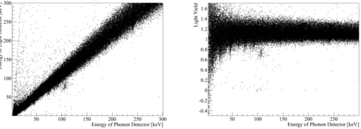
Figure 2.9.: The left plot shows the energy seen by the light detector on the y-axis over the energy seen by the phonon detector on the x-axis. The plot on the right side shows the light yield instead of the light on the y-axis. This light yield - energy plane is the common way to show CRESST data. The data is the same in both plots.

2.4. Light Yield and Quenching Factors

As discussed above, each event

²

contains information on the deposited energy in the phonon and the light detector. Most of the total energy of a particle interaction is deposited in the phonon detector, nearly independently of the type of particle. On the other hand the amount of scintillation light and therefore the energy measured in the light detector differs for different types of particles. The energy deposited in the light detector relative to the energy deposited in the phonon detector is quantified by the dimensionless light yield parameter:

light yield = energy deposited in light detector [keV

_ee

]

energy deposited in phonon detector [keV

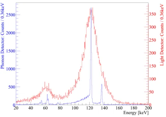
_ee

] (2.3) The index ee in the upper formula is an abbreviation for electron equivalent. Denoting the energy scale as electron equivalent is formally necessary, because the energy calibra- tion, which will be discussed in section 3.4, was done with electron recoils induced by 122 keV γ’s from a

⁵⁷

Co γ-source. This denomination is, in particular, important for the light channel because of the dependence on the type of interacting particle, as discussed before.

Figure 2.9 introduces the common light yield-energy plane (right side of the figure), which will be used several times in this work. By calibration γ- respectively electron interactions have a light yield of one

³

(at 122 keV) . It was found that nuclear recoils and α’s give less scintillation light than γ’s and hence have a lower light yield. This effect is quantified by the so-called quenching factor.

2

An event always encloses pulses from all detectors of a detector module.

3

The amount of scintillation light is not exactly identical for electrons and

γ’s ([20]). However, this

was discovered after the term

electron equivalent

was introduced.

(25)

2. The CRESST Experiment

Particle QF [%]

O 10.4 ± 0.5

α’s 22

Pb 1.4

Ca 6.38

^+0.62_−0.65

W 3.91

^+0.48_−0.43

Table 2.1.: Overview of relevant quenching factors for this analysis.

The quenching factor is defined as the ratio of the light output of a particle inter- action compared to a γ-interaction of the same deposited energy. Some of the needed quenching factors can be measured directly in data from the CRESST experiment. Since neutrons will scatter mainly off oxygen, a neutron calibration can be used to measure the quenching factor of oxygen. Such a calibration was performed during run 32. Fur- thermore, the quenching factors for lead and α’s were determined using corresponding events present in the Dark Matter data of run 32. However, other quenching factors require dedicated experiments

⁴

to measure them ([21]), because CRESST Dark Mat- ter data does not provide sufficient statistics. Table 2.1 gives an overview of the used quenching factors.

2.5. Resolution and Bands

Events of different types of particles will show up in different regions/bands in the light yield-energy plane. Each of these bands is defined by two functions. The first function describes the mean value of the light yield of an interaction of the corresponding particle as a function of energy. The second function, which is also energy dependent, describes the width of a band around its mean value. The width of the bands depends on the energy resolution of the light and phonon channel and is mostly dominated by the former.

The position and width γ-band is known very precisely due to the high statistics in the Dark Matter data. Therefore, the γ-band is used as a basis to calculate the quenched bands of the other event types. A more detailed description of the calculation of the bands can be found elsewhere (for example in [10]). An example for a light yield-energy plane with the bands plotted can be found in figure 2.10 . Usually bands are drawn such that in between the two boundaries of each band 80% of the events are expected (another 10% above and another 10% below). As one can see in figure 2.10 the bands broaden towards lower energies. This leads to overlaps between the different bands. However, in the overlap-free regions of the nuclear recoil bands it is possible to identify the recoiling nucleus by the information on the light yield of a certain nuclear recoil event.

4

In particular, measurements of the tungsten quenching factor are currently ongoing within the

CRESST collaboration at the

Technische Universit¨at M¨unchen. Furthermore Monte Carlo simu-

lations with the aim of determining the quenching factor of tungsten using CRESST data are under

development.

(26)

2. The CRESST Experiment

For this work the bands were fitted according to [10], where a detailed description of the whole procedure can be found. Since the energy resolution of the detectors will be used later in this work this aspect will be explained briefly in the next subsection.

2.5.1. Energy Resolution and the Width of the Electron/γ-Band

As discussed above, the width of the bands is dependent on the energy resolution of the detectors. Since the e/γ-band can be determined with high accuracy due to the large number of e/γ-events, the energy resolution of the detectors can be extracted from the fit of the e/γ-band. Since the resolution of the light channel is dominant it is reasonable to parametrize the measured width of the e/γ-band as a function of the amount of scintillation light L. According to [10] the e/γ-band can well be described by a Gaussian function of the width:

σ(L) = p

S

0

+ S

1

· L + S

2

· L

²

(2.4) The elements of above equation take the following contributions to the width of the band into account (The influence of the resolution of the phonon channel is neglected for now. Its influence will be discussed later.)

S

₀

is the baseline noise of the light signal.

S

₁

arises from the quantization of the energy, i.e. from the number of photons produced.

S

₂

takes other uncertainties into account which are proportional to L, for example a position dependence of the amount of scintillation light produced (further infor- mation can be found in [9]).

S

0

could, in principle, be determined by the fit of the e/γ-band. However, the resolu- tion of the test pulses provides a more precise measurement of S

₀

, because the test pulse resolution will only be affected by the baseline noise. Thus, the test pulse resolution was used to determine S

0

in this work and S

0

was fixed in the fit of the e/γ-band, whereas S

_1,2

were free fit parameters. In [10] it was shown that the resolution of the phonon de- tector has also to be taken into account and that S

₀

is then given by S

₀

= (σ

₀^l

)

²

+ (σ

^p₀

)

²

, with σ

₀^l

, σ

₀^p

being the test pulse resolutions of the light detector and the phonon detector, respectively.

2.5.2. Acceptance Region

The acceptance region is the region in the light yield-energy plane, in which possible

WIMP events are searched for. It is chosen module-wise. The upper limit of the accepted

energy range is set to 40 keV, common for all detectors. Above this energy nuclear

form factor effects ([22]) in combination with the rather low expected WIMP velocities

prevent an effective energy transfer on the nucleus and thus no significant WIMP signal

is expected for energies above 40 keV. The lower energy threshold of the acceptance

region is chosen such, that the expected leakage from the γ-band into the acceptance

(27)

2. The CRESST Experiment

Figure 2.10.: Shown is the light yield as a function of the energy deposited in the phonon detector for the detector module Verena & Burkhard & Q as presented in [1]. Highlighted are the bands were 80% of α (yellow), oxygen (cyan) and tungsten (gray) events are expected. Furthermore the acceptance region for this detector module is shaded in orange.

region is limited, for example to one event per module for the whole run in the latest

analysis. In the light yield coordinate the upper boundary of the acceptance region is

set at the upper boundary of the oxygen band. Towards lower light yields the lower

boundary of the tungsten band completes the definition of the acceptance region. The

calcium band is located in between the oxygen and the tungsten band and hence is also

part of the acceptance region. This definition of the acceptance region ensures that all

nuclei present in the CaWO

₄

target crystal can contribute, which makes the CRESST

experiment sensitive to a wide range of possible WIMP masses.

(28)

3. Data Preparation

3.1. Run 32

Run 32 was the first extensive physics run of the CRESST experiment and lasted from May 2009 until March 2011. Most of the measuring time was used to take Dark Matter data. However, two neutron calibrations and two γ-calibrations were also performed.

The CRESST setup has a capacity to house 33 detector modules. Table 3.1 gives an overview of the operational detector modules in run 32. Out of 18 installed modules, ten were fully operational, seven had problems with one detector and one module was not working at all.

As one can see in table 3.1 six light detectors could not be operated. This happened, because these detectors did not get cold enough for the TES to reach its superconducting transition.

The detector module ZnWO

₄

-4 & Ulrich was installed to test ZnWO

₄

as a target material and will not be used in the analysis. The module Zora & Yoichiro will also not be used for this Dark Matter analysis, because its exceptionally poor energy resolution leads to nearly no sensitivity to possible WIMP scatterings.

3.1.1. Blind Analysis and Data Sets

A central concept for any data analysis in the world of physics is the blind analysis. In general blind means, that not all information, which are necessary to get the final result of the analysis/experiment, are available for the analyst in order to avoid a conscious or unconscious influence towards the expected or desired result. Proceeding this way ensures a valid and objective analysis.

In this work a blind analysis was done by using a small subset of the Dark Matter data set as training set. All cuts and their parameters were developed on the training set and then applied without changes to the full data set. Table (3.2) gives an overview over the used data and training sets. Special data sets had to be used for the module K07 &

David, because David was not operational right from the start of run 32. The training

set of K07 & David was chosen such, that the live time respectively the exposure was

roughly the same as for the other detectors in their corresponding training set. The

raw exposure of all detectors (used for the Dark Matter analysis of this work) for the

training set was 79 kg d and 868 kg d for the Dark Matter data set.

(29)

3. Data Preparation

Phonon

Det. Light Det. Used for

Analysis ? Crystal Comment

1 VK33 Franz

yes CaWO

₄

2 Verena Burkhard,Q two light detectors

3 Maja Hans

4 Sabine Josef

5 Wibke X

6 Daisy SOS08

7 Rita Steven

8 K07 David D. not working at beginning

9 Zora Yoichiro

no

CaWO

₄

poor energy resolution

10 VK31 -

11 - Isaac

12 K14 -

13 VK34 -

14 Quedlina -

15 Yvonne -

16 ZnWO

₄

-4 Ulrich

ZnWO

₄

test module

17 ZnWO

₄

-6 - test module

Table 3.1.: An overview of all 17 detector modules with at least one operational detector in run 32. The first eight modules were used for the analysis. The others were only used to find coincidences.

Detector Modules Training Set Dark Matter Data Set

Files Raw Exp. [kg d] Files Raw Exp. [kg d]

1 VK33 & Franz

bck 22 - bck 72

9.8 bck 22 - bck 427

110 2 Verena & B. & Q 9.9 112

3 Maja & Hans 9.7 108

4 Sabine & Josef 9.8 108

5 Wibke & X 10.0 110

6 Daisy & SOS08 9.9 109

7 Rita & Steven 9.9 110

8 K07 & David bck 64 - bck 116

9.9 bck 64 -

bck 427

101 Total 79 868

Table 3.2.: This table lists the start and the end file of the training and data sets used

in this analysis. Furthermore the raw exposure (exposure before cuts) for each detector

module and the sum of all modules which were used for the Dark Matter analysis are

given in this table.

(30)

3. Data Preparation

Parameter Name Type Description Time Since Start [h]

E The elapsed time since the beginning of the data set.

Live Time [h] The effective live time during which the detector was in operation.

Pulse Height [V]

P

The pulse height is the height as determined us- ing a moving average over 50 channels. It is the difference between the highest obtained value in the record and the baseline level.

Peak Position [ms] The position in the record with the maximum signal (pulse height).

Pulse Onset [ms] The pulse onset is determined by going from the peak position backwards in time and finding the time, when the pulse started to rise above the baseline noise. Again an average over 50 channels is used.

Right - Left Baseline [V] The average of the last 50 channels in the record minus the average of the first 50 channels in the record are saved as the “Right - Left Baseline”

parameter.

Trigger Delay [ms] All detectors of a module can trigger a readout.

The first detector, which triggers in a digitizer module, has zero trigger delay. If the signal height in further detectors on the same digitizer module rises above trigger threshold the elapsed time is stored as “Trigger Delay”.

Table 3.3.: Main Pulse (P) and Event (E) Parameters.

3.2. Main Pulse and Event Parameters

An event contains pulses from the phonon and the corresponding light detector(s) of all detector modules on the same digitizer module, which registered a signal above the trigger threshold within a certain time window. An overview of the most important parameters of such an event and of the individual pulses in an event can be found in Table 3.3.

3.3. Standard Pulse Fit

Each type of pulses (particle and test pulses) is fitted with the corresponding template

(also called standard pulse). An example for such a fit can be seen in figure 3.1. The

aim of this fit is to determine the amplitude of each pulse as precise as possible, because

(31)

3. Data Preparation

Figure 3.1.: A pulse (red) fitted with a template (also called standard pulse - black).

The blue arrows indicate the possibility to move the template up or down, to shift it in time and to scale it.

the amplitude of a pulse is measuring the deposited energy and therefore the energy resolution will depend on the precision of the determination of the amplitude of the pulse. To fit the pulse with a template, instead of just using the “Pulse Height [V]”

parameter, has the following advantages:

• The pulse height parameter will in general overestimate the true height of the pulse, because the recorded signal in general is a superposition of the pulse and noise. Hence the maximum of a pulse will preferably be found at the position of a positive fluctuation of the noise. In contrast a negative noise excursion will not be taken into account.

• The energy of different events can only be measured by their pulse heights, if all

events have the same pulse shape. This is fulfilled for small pulses only, which

do not drive the TES outside its linear range. For pulses out of the linear range

the pulse height is not a well suited parameter any more. Furthermore, the max-

imum pulse height, which can be measured by a TES, is given by the end of the

superconducting transition for the corresponding TES. Therefore the pulse height

parameter will be roughly the same for all events above a certain energy deposi-

tion. In conclusion the pulse height can only be used for small pulses in the linear

range of the TES. In contrast the template fit also allows to measure the energy

(32)

3. Data Preparation

Figure 3.2.: On the left side the RMS of the standard pulse fit is plotted over the amplitude of the fit for a large number of pulses. The increase of the RMS starting for amplitudes above 2.62 V is a consequence of the pulse shape changing when leaving the linear range of the transition of the detector. Therefore, the parts of the pulse above this so called truncation level are not well described by the template. Thus, only data below the truncation level are included in the fit. Such a truncated fit is shown in the right plot.

deposition of much larger pulses (will be discussed below).

For particle pulses a standard pulse can be generated from either calibration sources or intrinsic radioactivity. To build a template it is important to use low energy interactions in the linear range of the detectors. In this work all standard events were acquired by averaging over pulses from the 122 keV line of a

⁵⁷

Co source, except for the detector David. Since David was not working during the calibration run (which was performed at the beginning of run 32) the template had to be generated out of the 46 keV line of the intrinsic

²¹⁰

Pb contamination.

A dependence of the trigger time on the pulse height is called trigger walk. To avoid trigger walk effects only events of a very small pulse height range were used to create a template. This is possible, because a few ten events are sufficient to build a standard event (which is shown in [9] on page 97.) Normally some hundred events were used in this work. The big advantage of creating a standard pulse out of a few hundred pulses, compared to just using a single particle pulse, is the cleanliness in terms of noise, because the noise is reduced by averaging.

Analysis of CRESST Dark Matter Search Data

PHYSIK-DEPARTMENT