Time-correlated Background and Background Mitigation Strategies in the KATRIN Experiment

(1)

Time-correlated Background and Background Mitigation Strategies in

the KATRIN Experiment

Master thesis at the faculty of physics of the

Ludwig-Maximilians-Universität München

submitted by

Alessandro Schwemmer born in Neustadt an der Waldnaab

Munich, 13.10.2020

(2)

(3)

Zeitlich korrelierter Untergrund und Strategien zur

Untergrundunterdrückung im KATRIN Experiment

Masterarbeit an der Fakultät für Physik der

Ludwig-Maximilians-Universität München

vorgelegt von

Alessandro Schwemmer

geboren in Neustadt an der Waldnaab

München, den 13.10.2020

(4)

(5)

Abstract

The Karlsruhe Tritium Neutrino (KATRIN) experiment aims at measuring the neutrino mass with a sensitivity of0.2 eV (90 %C.L.)in a model independent way. To this end it uses electrons originating from tritiumβ-decay and investigates their spectrum close to the kinematic endpoint. In order to reach the desired sensitivity a low background and a good understanding of its properties is necessary. This thesis presents a data-driven Monte Carlo simulation of the background focusing on its non-Poissonian nature which originates from nuclear decays in the main spectrometer. The impact of a non-Poisson background on the neutrino mass under various model assumptions and measurement congurations is investigated. It could be shown that dierent scanning strategies and background treatments have a minor impact on the neutrino mass result. Furthermore optimising the electromagnetic eld conguration in the main spectrometer allows for an overall background reduction by a factor of 2. However this asymmetric setting requires precise measurements of the electromagnetic elds in the center of the spectrometer. In the scope of this thesis a new method of eld calibrations with a gaseous krypton source has been established and the eld input values for the third neutrino mass campaign were provided.

(6)

(7)

Zusammenfassung

Das Ziel des Karlsruhe Tritium Neutrino (KATRIN) Experiments ist die Messung der Neu- trinomasse mit einer Sensitivität von0.2 eV (90 %C.L.) in einer modelunabhängigen Art und Weise. Dazu nutzt es Elektronen aus dem Tritiumβ-Zerfall und untersucht deren Spektrum nahe des kinematischen Endpunkts. Um die gewünschte Sensitivität zu erreichen, ist ein niedriger Untergrund sowie dessen gutes Verständnis notwendig. Diese Arbeit stellt eine auf Daten basierte Monte Carlo Simulation des Untergrunds vor und konzentriert sich dabei auf dessen Abweichung von einer Poisson Verteilung, was seinen Ursprung in Kernzerfällen im Hauptspektrometer hat. Die Auswirkung dieses non-Poisson Untergrunds auf die Neutri- nomasse wurde unter verschiedenen Modellannahmen und Messkongurationen untersucht.

Es zeigte sich, dass unterschiedliche Scanstrategien und Untergrundbehandlungen zu einer kleinen Auswirkung auf die Neutrinomasse führen. Weiterhin erlaubt eine Optimierung der elektromagnetischen Felder im Hauptspektrometer die Reduzierung des totalen Untergrunds um einen Faktor 2. Diese asymmetrische Konguration erfordert jedoch präzise Messungen der elektromagnetischen Felder im Spektrometer. Im Rahmen dieser Arbeit wurde eine neue Methode zur Feldkalibrierung mit einer gasförmigen Kryptonquelle herangezogen und Feldw- erte für die dritte Messung der Neutrinomasse wurden angegeben.

(8)

(9)

The neutrino

Despite being one of the most abundant particles in the universe, there are still open questions concerning the neutrino. Due to its weak interactions with other particles and its small mass, it took many years from its prediction to evidence of its existence. And still today the neutrino oers room for discussion. This chapter describes briey the neutrino's history, its description in the standard model (SM) of particle physics and the implications of neutrino oscillations on the SM. For better readability this thesis uses natural units (~=c= 1).

1.1 History of discovery

The motivation for the neutrino was coming from J. Chadwick's investigations of the β- spectrum in the early 20^thcentury. As αandγ-spectra showed discrete lines representing the energy dierence between the nuclei, the continuousβ-spectrum was not understood in the rst place [1]. At this time, theβ-decay was thought to be a two-body-decay: The nucleus emits an electrone⁻ and a protonp, their energy is dictated by energy-momentum-conservation, i.

e. the spectrum should be discrete.

This discrepancy between theory and experiment lead W. Pauli to the proposal of a new particle, now known as the neutrinoν. As charge is conserved, this particle should be neutral, but not a photon as this could be easily detected [2].

Building up on the idea of this postulated particle, E. Fermi formulated his theory ofβ-decay:

A neutron n in the nucleus decays into a proton, an electron and a (anti-)neutrino ν¯ (see eq. (1.1)). In this three-body-decay, the individual energies of the particles in the nal state are not xed, therefore the spectrum is continuous [3].

n→p+e⁻+ ¯νe (1.1)

Between the theoretical postulate of the neutrino and its discovery over 20 years passed. The conformation took place in 1956, done by C. L. Cowan and F. Reines. They used a nuclear ssion reactor as (potential) neutrino source. Those neutrinos reacted with protons in a target tank, producing positrons and neutrons, see eq. (1.2). In this case, the signal consists two energy depositions. The prompt one being twoγ photons originating from the annihilation of the positrone⁺. The delayed energy deposition is caused by cadmium capturing the neutron n and releasing a γ photon (see e.g. eq. (1.3)). A signal to background ration of 3 to 1 and signal dependence on the reactor power lead to the conclusion that the signal is indeed induced by a neutrino [4, 5].

νe+p→n+e⁺ (1.2)

113Cd +n→¹¹⁴Cd +γ(9.2 MeV) (1.3) 1

(12)

1.2 Description in the standard model of particle physics

The standard model (SM) of particle physics describes all known particles and interactions with high precision. It characterises the neutrino as a massless, uncharged lepton. Interactions between the neutrino and other particles are mediated via the weak force. This only involves left-handed neutrinos. Right-handed neutrinos either do not exist or interact exclusively via gravitation. In the framework of electroweak theory, left-handed leptons are grouped in doublets in accordance with their (weak) isospin as shown in eq. (1.4) for the three generations.

As right-handed leptons do not interact via charged currents¹and hence have no isospin, they form singlets as given in eq. (1.5). A very similar procedure holds for quarks, but is not presented here. Therefore the electroweak interaction aects all fermions [6].

νe

e⁻

L, νµ

µ⁻

L, ντ

τ⁻

L (1.4)

e⁻_R,µ⁻_R,τ_R⁻ (1.5)

Charged currents are described by massive gauge bosons denoted as W^±. As their mass is O(80 GeV)Fermi's theory that does not include these bosons is valid at low energies in which case the interaction is reduced to a single point. An example of a possible interaction is shown in g. 1.1, the handedness is not shown explicitly.

W⁻

d

u νe

e⁻

Figure 1.1: Example of a charged current.

Furthermore leptons obey another conservation law. Each lepton is assigned a lepton number, being 1 or −1 for particles or anti-particles respectively. This number is conserved globally and in particular for each individual generation. Violations of this number have so far only observed in the context of neutrino oscillations. This will be explored in the next section [7].

1.3 Neutrino oscillations and their implications

In 1968, R. Davis Jr. conducted his famous Homestake experiment to search for neutrinos from the sun: A tank lled which liquid tetrachloroethylene served as the detector. Incom- ing electron neutrinos react with the chlorine and produce argon, together with an electron (eq. (1.6)). The produced argon is removed from the tank and its decays allow for an estima- tion of the previous production, hence for theν_eux. The observed ux coming from the sun is signicantly smaller than expected from theoretical predictions [8]. This marks the rst hint to neutrino oscillations.

37Cl +νe→³⁷Ar +e⁻ (1.6)

1As the distinction suggests there are also neutral currents, which are not covered here. Please refer to [6].

(13)

1.3. NEUTRINO OSCILLATIONS AND THEIR IMPLICATIONS 3

In the following years various experiments have shown avour changes of neutrinos travelling over large distances. Looking at atmospheric neutrinos induced by cosmic rays have shown evidence for neutrino oscillations, in good agreement with the two-avour oscillation hypoth- esis, see eq. (1.7). In this simplied model, the probability for a neutrinoν_a to oscillate and be observed in a dierent avor state νb after travelling a distance L depends on its energy E_ν, the mixing angle θand the mass squared dierence ∆m² [9].

P(ν_a→ν_b) = sin²(2θ)·sin²

1.27∆m²(eV²)L(km) Eν(GeV)

(1.7) Since the oscillations would disappear for vanishing∆m², this implies that not all neutrinos can be massless. As described in section 1.2, there are three generations, i.e. three avors of neutrinos. In general oscillations between every pair of them are possible. To account for their masses, three mass eigenstatesν_i,i∈ {1,2,3} are introduced which mix with the weak eigenstatesνl,l ∈ {e, µ, τ}, see eq. (1.8). The strength of the mixing is parametrised by the matrix elementsU_li [7, 10].

|ν_li=X

i

U_li|ν_ii (1.8)

However neutrino oscillations are only sensitive to mass squared dierences. For a direct neutrino mass measurement, a dierent type of experiment is needed. This is described in the following section.

(14)

(15)

Chapter 2

The KATRIN Experiment

The Karlsruhe Tritium Neutrino (KATRIN) experiment aims at measuring the neutrino mass in a direct, model independent fashion. Similar to its predecessors in Mainz [11] and Troitsk [12], its observable is the eective anti-neutrino massm(νe):

m(ν_e) = v u u t

3

X

i=1

|U_ei|²m²_i (2.1)

After three years of data taking, KATRIN is designed to have a sensitivity ofm(ν_e)≡m_ν = 0.2 eV at 90 %condence level (C.L.) [13].

Section 2.1 gives an overview of the tritiumβ-decay used for the neutrino mass determination, followed by a short description of the measurement principle in section 2.2. The model of the integral tritium spectrum is given in section 2.3 while the data modelling tool is presented in section 2.4. A short experimental overview is presented in section 2.5. This chapter is concluded with results from the rst neutrino mass measurement campaign in section 2.6.

2.1 Tritium β-decay

In order to measure the neutrino mass m_ν as dened in eq. (2.1), KATRIN uses electrons coming from theβ-decay of Tritium:

3H→³He⁺+e⁻+ ¯ν_e (2.2)

The neutrino mass would manifest itself in a distortion of the spectrum (see g. 2.1), which would be visible mostly near the endpoint E₀, the maximal energy of an electron assuming mν = 0 eV [13]. The dierential decay rate of tritium can be described using Fermi's Golden Rule. One obtains eq. (2.3). F(Z, E) represents the Fermi function describing Coulomb interaction between the electron and the nucleus in the nal state having an atomic charge Z. E,p and me refer to energy, momentum and mass of the electron respectively whileΘ is the Heaviside function guaranteeing energy conservation. The constantC⁰ is given in terms of the Fermi constant G_F, the Cabibbo angle θ_C and the nuclear transition matrix element M_nuc (see eq. (2.4)) [14, 15].

dΓ

dE =C⁰·F(Z, E)·p·(E+m_e)·(E₀−E)·p

(E₀−E)²−m²_ν ·Θ(E₀−E−m_ν) (2.3) C⁰ = G²_Fcosθ_C²

2π² · |M_nuc|² (2.4)

5

(16)

18571 18572 18573 18574 18575 Electron energy (eV)

0.0 0.5 1.0 1.5 2.0 2.5

Rate (cps / eV)

1e 20

m = 0 eV m = 1 eV m = 2 eV

Figure 2.1: Eect ofmν on the tritium spectrum near E0 [14].

For a precise modelling, further modications of the dierential spectrum become necessary.

This includes but is not limited to the thermal induced Doppler eect or the distribution of molecular nal states, see [14, 15].

2.2 MAC-E lter

Following the success of the Mainz and Troitsk neutrino mass experiments, KATRIN uses a magnetic adiabatic collimation combined with an electrostatic lter (MAC-E lter) in its spectrometers. This lter combines the needed high energy resolution with high luminosity [13].

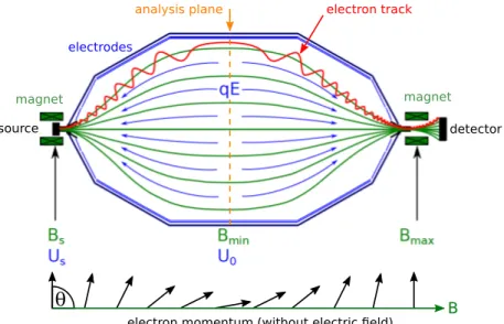
The β-electrons coming from the source are guided by magnetic eld lines through the spectrometer, as sketched in g. 2.2. On their way they perform cyclotron motion around the eld lines, resulting in an acceptance angle of up to 2π. Due to the magnetic mirror eect this angle however is limited and usually around 50° in KATRIN [13].

As the electrons move through the spectrometer the B-eld drops by several orders of magnitude until it reaches its minimum B_min, dening the analysing plane (AP). Because of the gradient in the magnetic eld, cyclotron motion is converted into longitudinal motion, shown in the bottom of g. 2.2 [13].

The electric potential is maximal in the AP, thus this conversion of longitudinal electron momentum enables electrons that start with an non-zero pitch angle θ w.r.t. the magnetic eld lines to overcome the potential barrier, despite having not enough longitudinal energy in the rst place.

Altogether this lter acts as an integrating high-energy pass lter with its energy resolution being determined solely by the magnetic elds:

∆E

E = B_min

B_max (2.5)

withB_min and B_max being the minimal and maximal magnetic eld respectively [13].

(17)

2.3. MODEL OF THE INTEGRALΒ-SPECTRUM 7

detector source

magnet magnet

electrodes

electron track

θ B

electron momentum (without electric ﬁeld) analysis plane

Figure 2.2: Top: Sketch of a MAC-E lter. Electrons (red) coming from the source are adiabatically guided through the spectrometer, performing cyclotron motion along the magnetic eld lines (green). If their energy is high enough to surpass the potential barrier introduced by the electrodes (blue), the electrons are re-accelerated towards the detector as they passed the analysing plane (AP) (orange dashed), where the electric potential is maximal and the magnetic eld is minimal. Bottom: Because of the magnetic eld gradient, the electrons cyclotron motion is converted into longitudinal motion while approaching the AP [16].

2.3 Model of the integral β-spectrum

The integralβ-decay spectrum consists of multiple parts. The dierential spectrum given in section 2.1 is combined with the experimental response of KATRIN presented in section 2.3.1.

Subsequently additional modications to account for background, thermal Doppler broadening and other eects are applied (see section 2.3.2).

2.3.1 Response function

As described in the previous section, KATRIN uses a MAC-E lter, resulting in an integrating high-energy pass lter. Therefore only electrons having sucient (longitudinal) energy can reach the detector. This property is encoded in the response functionR(qU, E) which gives the probability for an electron with energyE to pass the MAC-E lter with xed retarding energyqU. Ideally, this would be a simple step function as given in eq. (2.6) [14].

R_ideal(qU, E) =

(0, ifE < qU

1, ifE ≥qU (2.6)

However the MAC-E lter does not convert all transversal energy into longitudinal energy.

Therefore even electrons with a total energy larger than the retarding energy may not overcome the potential barrier. Following eq. (2.5) a normalized relativistic transmissionT(qU, E) function can be derived, describing the electron transmission probability:

T(qU, E) =











0, if E < qU

1−

r 1−f· ^B^S

Bmin·^E−qU

E

1−

q 1−_B^BS

max

, if qU ≤E ≤qU_f·B^f·B^max

max−B_min

1, if E > qU_f_·B^f^·B^max

max−B_min

(2.7)

(18)

with q being the electric charge of the particle, E its total energy, qU the retarding energy and f a relativistic factor given by eq. (2.8) [14]. The shape of the transmission is shown in g. 2.3a. For B_min = 0, the transmission would resemble a simple step function like for an ideal high-pass energy lter.

f =

E−qU me + 2

E

me + 2 (2.8)

Due to scattering of electrons with tritium molecules in the source the transmission function has to be modied. To this end the energy loss in each scattering process is included by convolving the transmission with the corresponding scattering probabilities and their energy loss function. Thus one obtains the KATRIN response function R(qU, E), shown in g. 2.3b [14].

0 1 2 3 4 5

E qU (eV) 0.0

0.2 0.4 0.6 0.8 1.0

Transmission probability

(a) Transmission

0 10 20 30 40 50

E qU (eV) 0.0

0.2 0.4 0.6 0.8

Transmission probability

(b) Response

Figure 2.3: Transmission probability and response function. The latter includes scattering of electrons in the source [14].

2.3.2 Integral spectrum

Combining the previously discussed response function R(qU, E) and the dierential decay spectrum _dE^dΓ(E) from section 2.1 gives the integral spectrum I(qU) of KATRIN. It is calculated via a convolution as given in eq. (2.9). Additionally a constant background rate B is added. The number of tritium atoms N_e, the acceptance angle θ_max and the detection eciency_detector are absorbed in C (see eq. (2.10)). Details are given in [14].

Γ(qU) =I(qU) +B =C· Z E0

qU

dΓ

dE(E)·R(qU, E) dE+B (2.9) C =N_e·1−cosθ_max

2 ·_detector (2.10)

2.4 Fitrium software

Fitting and modelling the data obtained in KATRIN is done using Fitrium. It includes, amongst others, the (integral) tritium model described in section 2.3 and a model for conversion electrons from krypton (see section 5.2.1). Currently Fitrium is maintained and developed by Christian Karl and Martin Slezák. It oers the capability to t a spectrum, but also to perform Monte Carlo (MC) simulations and to propagate systematic uncertainties [14].

(19)

2.5. EXPERIMENTAL OVERVIEW 9

Fitting a spectrum is done via a maximum likelihood analysis. To this end, a likelihood functionL is dened:

L=L(µ(~θ);x) =L(θ;~ x) (2.11) This likelihood function describes the probability for a model µ with parameters ~θ to be realised given the data from experimentx. It is maximised by nding the optimal parameters decoded in~θto describe the data. To this end the negative logarithmic likelihood is minimised, which is given in eq. (2.12) and related to theχ²(dened in eq. (2.13)) for Gaussian distributed data [14].

−lnL(µ;x) = 1

2χ²(µ;x) (2.12)

χ²(µ;x) =X

i

(x_i−µ_i)²

σ_i² (2.13)

Herex_idenotes the data points that are compared to their model expectationµ_i and weighted by their uncertaintyσi.

Systematic uncertainties like the magnetic elds can easily be included by modifying the likelihood function with a pull-term (also called nuisance parameter). Typically this means a multiplication with a Gaussian (see appendix B.2) that constrains the systematic parameter in terms of its expectation value and uncertainty. However this leads to increased computational eort as the systematic parameter is an additional parameter that needs to be optimised [14].

A dierent approach is to use covariance matrices. In this case theχ² is dened to be χ²(µ;x) = (µ−x)^|V⁻¹(µ−x) (2.14) with V being the covariance matrix. In addition to statistical uncertainties, systematics are included by calculating multiple model spectra sampling the systematic parameters from their distribution. The covariance matrix is then calculated from these model spectra.

A third possibility is to repeat the t instead of calculating a model spectrum. This is done in the framework of MC propagation and leads to a distribution of the t parameter(s) which is broadened w.r.t. a statistics only case. For a detailed discussion of the tting procedure and the treatment of systematic uncertainties, please refer to [14].

2.5 Experimental overview

The length of the KATRIN experiment is70 m. Its beamline, shown in g. 2.4, unies dierent components described in the following. Each part serves a dierent, unique purpose.

2.5.1 Rear Section

The rear section mainly serves as a calibration and monitoring system. It consists of a gold- plated stainless-steel disk with a central aperture of5 mm, allowing to sent electrons or ions through the beamline. As the electrons are coming from a photo-electronic source, their energy and pitch angle w.r.t. the magnetic eld is well dened, thus allowing for measurement of the response function (see section 2.3.1) and other systematic eects. The rear wall (RW) itself can be used to characterise the plasma and avoid distortions of the spectrum induced by additional potentials [17, 18].

(20)

Figure 2.4: KATRIN beamline:

a) Rear section

b) Windowless gaseous tritium source (WGTS) c) Dierential pumping section (DPS)

d) Cryogenic pumping section (CPS) e) Pre-spectrometer (PS)

f) Main spectrometer (MS) g) Focal plane detector (FPD) 2.5.2 Windowless Gaseous Tritium Source

The10 mlong windowless gaseous tritium source (WGTS) houses the tritium molecules deliv- ering up to10¹¹β-decay electrons per second as long as KATRIN is operating in usual tritium mode. The gas is cooled down as low as27 Kand has a high isotopic purity (>95 %). It is in- serted through a set of capillaries in the middle. By controlling the gas injection pressure, the column density ρd of the WGTS can be adjusted w.r.t. its reference value of5×10¹⁷cm⁻². The produced electrons are adiabatically guided through the source using a magnetic eldBS

until reaching the end of the tube [13].

2.5.3 Transport Section

As theβ-electrons reach the end of the WGTS tube they are supposed to enter the spectrometer. In order to avoid tritium doing so as well, leading to elevated spectrometer background, the transport section consists of the dierential pumping section (DPS) and the cryogenic pumping section (CPS).

The DPS uses turbomolecular pumps in order to reduce the gas-ow by at least ve orders of magnitudes. The electrons are guided adiabatically through this section, while neutral molecules hit the beamtube which is composed of tilted neighbouring elements. Tritium- containing ions are removed using a ring electrode and electric dipole elements.

Subsequently the CPS reduces the tritium ow by additional seven orders of magnitude using cold traps. Similar to the DPS tritium molecules strike the wall due to a tilt of beamtube segments. As the wall consists of a 3 K argon-frost layer which provides a higher binding energy than normal cryo-condensation, tritium molecules are adsorbed.

After passing this section, the electrons may enter the spectrometer while the gas-ow has been reduced by about10¹² [18].

2.5.4 Pre- and Main Spectrometer

Both spectrometers are based on a MAC-E lter as described in section 2.2. The PS is operated at xed retarding potential, thus acting as a pre-lter. This minimises background coming from ionization of residual gas molecules in the MS. The MS itself scans theβ-spectrum using dierent retarding energies close to the endpoint E₀. To suppress the background

(21)

2.6. FIRST NEUTRINO MASS MEASUREMENT CAMPAIGN 11

further, it has an inner electrode (IE) at slightly more negative potential. This way low- energy electrons or ions emanating from the inner surface of the vessel may not enter the ux tube. To avoid scattering on residual gas, the pressure in the pre- and main spectrometer is only1×10⁻¹¹mbar[13].

2.5.5 Focal plane detector

The FPD completes the KATRIN beamline. It is a multi-pixel silicon diode array, segmented in 148 pixels as shown in g. 2.5. All pixels have the same surface area. Electrons coming from the MS are accelerated by10 kV using a post-acceleration electrode (PAE). This PAE allows for additional background reduction, induced by for instanceβ- and γ-emitting nuclei close to the detector [13, 18].

1 0

2 3 4

5 7 6 8 9

10

11

12 13 14

15 16 17 19 18

20 21

22

23

24 25

26 27

28

29 31 30

32 33

34

35

36 37

38 39

40 41 43 42

44

45

46

47

48 49

50 51

52

53 54 55 56

57

58

59

60 61

62 63

64 65 67 66

68

69

70

71

72 73

74 75

76

77 78 79

80

81

82

83

84

85

86 87

88 89 91 90

92

93

94

95

96 97

98 99

100

101 102 103

104

105

106

107

108

109

110 111

112 113 115 114

116

117

118

119

120 121

122 123

124

125 126 127

128

129

130

131

132

133

134

135 136 137 139 138

140

141

142

143

144 145

146 147

Figure 2.5: Segmentation of the focal plane detector. The pixels are labelled counter-clockwise from inside to the outside.

2.6 First neutrino mass measurement campaign

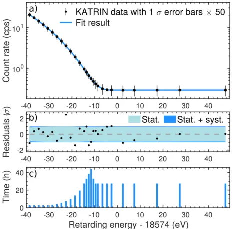
The rst neutrino mass measurement campaign called KATRIN neutrino mass 1 (KNM1) took place in spring 2019. The integral tritium β-decay spectrum is scanned multiple times.

Each scan lasts about2 hand consists of various subscans at dierent retarding energiesqU. For one subscan the retarding energy is xed and electrons reaching the detector are counted for a certain amount of time. The spent time for each retarding potential is higher in the region close to the tritium endpoint E0 as the distortion due to mν is maximal there (see g. 2.6 c) [19].

In total274scans are selected based on data quality criteria. Those scans are then stacked at hqUifor each subscan. For further analysis, noisy and shadowed pixels are excluded and 117 pixels are used when tting the data. The corresponding spectrum and the best-t model are

(22)

-40 -30 -20 -10 0 10 20 30 40 10⁰

10¹

Count rate (cps)

KATRIN data with 1

a) error bars 50

Fit result

-40 -30 -20 -10 0 10 20 30 40

-2 0 2

Residuals()

Stat. Stat. + syst.

-40 -30 -20 -10 0 10 20 30 40

Retarding energy - 18574 (eV)

0 20 40

Time (h)

b)

c)

Figure 2.6: a) Integral spectrum of electrons after stacking 274scans. The uncertainties are enlarged by a factor of 50. The best-t model is also shown. b) Residuals normalized w.r.t.

the 1σ uncertainty band. c) Total measurement time for all retarding energies. Figure from [19].

shown in g. 2.6 a). Displayed errorbars are enlarged by a factor of 50 for better readability.

The data is well described by the model covered in section 2.3.2. The residuals shown in g. 2.6 b) indicate a very good t and highlight the dominance of statistical uncertainties.

The model consists of four free parameters: The neutrino mass squared m²_ν, the background rate B, the endpoint E₀ and an additional amplitude similar to C in eq. (2.9). Systematic uncertainties are propagated using MC propagation or a covariance matrix approach. An overview of the systematic uncertainties is given in g. 2.7. For KNM1 the non-Poisson (NP) background was an important systematic uncertainty. Details of the background model and the implications are discussed in chapter 3. Finally a best-t value of the neutrino mass squared can be given as in eq. (2.15). Using the methods of Lokhov and Tkachov an upper limit on the neutrino mass is obtained in eq. (2.16), which is the central result of KNM1 and has improved the limits of KATRIN's predecessors by a factor of 2[19].

m²_ν = (−1.0^+0.9_−1.1) eV² (2.15)

m_ν ≤1.1 eV (90 %C.L.) (2.16)

(23)

2.6. FIRST NEUTRINO MASS MEASUREMENT CAMPAIGN 13

0.00 0.05 0.10 0.15 0.20 0.25 0.30

1- uncertainty on m² (eV²) ELoss

FSD Stacking B-fields d Background slope

Non-Poisson bkg.

0.044 0.049 0.052 0.066 0.298

Figure 2.7: Systematic uncertainties for KNM1. Plot by Christian Karl.

(24)

(25)

Chapter 3

Background

Generally speaking all electrons created in the ux tube of the MS can contribute to the overall background. Electrons from the PS are blocked by the retarding potential which is higher in the MS compared to the PS. The overall background is mainly Rydberg induced as explained in section 3.1. Additionally two contributions arise from radon decays in the main spectrometer and intrinsic detector background [20]. These are presented in section 3.2 and section 3.3 respectively. Other minor sources of background processes are discussed in [20].

This chapter is concluded with a simple way to characterize the background.

3.1 Rydberg-induced background

The main source of background is coming from low-energy electrons being created in the MS.

This is sketched in g. 3.1. As the inner wire electrodes (see section 2.5.4) prevent charged particles from entering the ux tube volume, only neutral atoms can do so. If those atoms are subsequently ionized, this can be a source of background [20].

The underlying processes are radioactive decays occurring in the walls. Those decays can lead to sputtering of neutral atoms, which eventually enter the ux tube volume. Being ionized by thermal radiation, this can lead to low-energy electrons being created. This requires the neutral atom being in a highly exited state (Rydberg state), as the energy of black-body radiation in the MS, which is at room temperature, is otherwise not sucient. This typically leads to electrons having energies below100 meV [20].

Low-energetic electrons are guided along the magnetic eld lines and accelerated by the retarding potential. This makes them indistinguishable from electrons originating from tritium β-decay. Furthermore this background mechanism scales with the volume between the analysing plane and the detector, hence decreasing this volume could lead to a reduction of this background [20].

3.2 Radon-induced background

While providing high energy resolution and luminosity, one drawback of the MAC-E lter is its equivalence to a magnetic bottle. As on both ends of the MS (see g. 2.2) the magnetic eld is large, charged particles can be trapped. Electrons created in the ux tube are guided by the magnetic eld on the one hand, and accelerated by the retarding potential on the other hand. On their way to one of the regions with high magnetic eld their longitudinal energy is transferred into transversal energy, as indicated in the bottom of g. 2.2. If the complete longitudinal energy is transferred, the electron is reected. This leads to a storage of electrons

15

(26)

IE

Thermal radiation Rydberg atom

Nuclear decay

Ionisation e⁻

Figure 3.1: Simplied cross section of the main spectrometer. Nuclear decays in its wall can lead to sputtering of highly excited, neutral atoms (Rydberg atoms). Charged particles are blocked by the inner electrode (IE). Rydberg atoms can subsequently be ionised by thermal radiation, creating low energetic electrons [20].

created at position x if eq. (3.1) is fullled [20].

E⊥> U_ret(x)· B(x)

B_max (3.1)

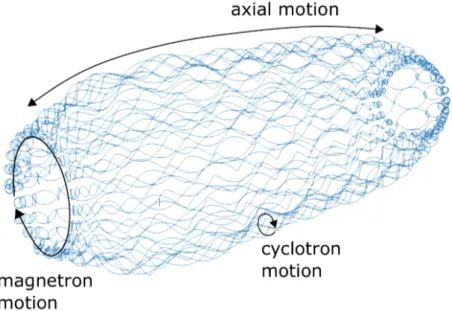
Therefore electrons with transversal energy larger than the energy resolution of the spectrometer are stored. The motion of a stored electron, as shown in g. 3.2, consists of axial, cyclotron and magnetron motion. As the radius of cyclotron motion increases linearly with transversal velocity, electrons with higher energy (O(100 keV)for usual magnetic eld settings) have radii larger than the spectrometer radius. These electrons hence collide with the walls and are not stored [20].

Trapped electrons however follow the motion given in g. 3.2 until breaking the storage condition. The storage time of such an electron depends mainly on the pressure: Due to scattering with residual gas, it loses energy and changes its momentum, thus eq. (3.1) eventually is not fullled anymore and the electron leaves the spectrometer either towards the detector or the source. Secondary electrons created by scattering processes usually leave the spectrometer immediately, being a contribution to the background. As these scattering processes are correlated to some extent, the events are not Poisson distributed [20]. This deviation is a large systematic uncertainty and played an important role in the rst neutrino mass measurement [19].

Since the storage condition eq. (3.1) requires a certain amount of (transversal) energy, trapped electrons arise mainly from radon decays. As the MS is continuously pumped out, only radon isotopes with short half-life decay in the ux tube volume. These decays happen homoge- neously distributed in the spectrometer. The radon atoms mainly come from the wall where they accumulated before assembly due to natural radioactivity. Furthermore non-evaporable getter (NEG) strips being intended to remove potential residual tritium emanate radon. ²¹⁹Ra for instance decays in an α-decay. Subsequently electrons are emitted having energies in the range of 1×10⁻³keVto 1×10²keV. A detailed discussion of the various processes is given in [20].

(27)

3.3. DETECTOR BACKGROUND 17

Figure 3.2: Motion of an electron trapped in the spectrometer. It is composed of axial and cyclotron motion along and around the magnetic eld lines respectively. Additionally eld inhomogeneities lead to magnetron motion [20].

Each emitted electron that is stored in the spectrometer undergoes scattering with residual gas. This leads to multiple secondary electrons, depending on the energy of the primarily stored particle as given in eq. (3.2) [20].

N_secondary≈ E_primary

hE_lossi (3.2)

hE_lossi denotes the average energy loss for ionisation while E_primary is the energy of the primarily stored electron. For primary electrons with energies of O(keV) this can lead up to O(100) secondary electrons [20].

3.3 Detector background

The detector background is dened to be present even if there is no connection to the MS.

It mainly consists of events following radioactive contaminations of the materials or cosmic rays. To minimise this background, the post-acceleration electrode is used in order to shift the signal to regions of lower intrinsic background. Using a muon scintillator can in principal further reduce this background, but as it is small compared to the Rydberg component this is currently not implemented in the analysis [13, 20].

3.4 Background characterisation

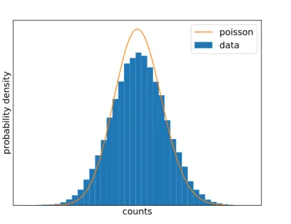
Disentangling the dierent background components described in the previous sections is a te- dious task. The scope of this work however is concentrated on the distinction between Poisson and non-Poisson (NP) background. To this end two simple variables are dened to quantify the deviation of the background distribution from a Poisson distribution (see appendix B.1).

Either a relative approach (eq. (3.3)) or an absolute one (eq. (3.4)) is used, depending on ensuing calculations or interpretations. The underlying idea is that time-correlated background leads to a broader distribution of the binned background, as sketched in g. 3.3. Hence the

(28)

counts

probability density

poisson data

Figure 3.3: Broadening of time-binned background distribution.

measured standard deviation σ is larger than the expected one given by the square root of the mean λ.

f_NP= σ

√λ−1 (3.3)

σ_NP=p

σ²−λ (3.4)

Whilef_NP has no unit,σ_NPreects counts hence dividing it by the time t_binused for binning one obtains a quantity usually given in counts per second (cps).

Both f_NP and σ_NP are zero for no NP component and related via eq. (3.5) with the total background rater =λ/t_bin.

σ_NP t_bin =

r r t_bin

p(f_NP+ 1)²−1 (3.5)

(29)

Chapter 4

Monte Carlo background simulation

So as to get a good understanding of the background and in particular its NP component, simulations based on data are performed. In this chapter, a description of the implemented simulation will be given in section section 4.1, followed by its experimental input in section 4.2.

Results are presented in section 4.3, eects on the neutrino mass sensitivity are discussed in section 4.4.

4.1 General concept

The MC simulation aims at reproducing the NP characteristic. To this end the total background is divided in two components, one being Poisson distributed and the other representing nuclear decays thus not being Poisson distributed. As for the latter the emitted electrons are stored, additional information about their storage time and the number of secondary electrons they create is needed. Summarizing this, the MC simulation takes the following inputs:

Poisson rate

rate of nuclear decays

storage times

numbers of secondary electrons

In order to simulate the background and in particular its NP component, the simulation is time-based. After specifying a total time and the step size of individual time bins, the following procedure is repeated for each time step as sketched in g. 4.1:

1. Draw a random number from a Poisson distribution. The expectation value is calculated from the Poisson rate and the size of the time bin.

2. Similar to step 1 draw another random number based on the rate of nuclear decays. As the nuclear decays itself are independent, they follow a Poisson distribution. For each nuclear decay in this time step, repeat the following sub steps:

(a) Choose a storage time and the corresponding number of secondary electrons ran- domly. Calculate the rate of the secondary electrons for this particular nuclear decay, being represented as a cluster. The storage time is hence interpreted as the time for all secondary electrons to hit the detector.

19

(30)

time Poisson Non-Poisson Cluster

Figure 4.1: Working principle of the MC simulation. In each time bin events coming from a Poisson process are drawn. Subsequently, following experimental inputs, clusters representing nuclear decays are drawn and their induced events are distributed. The starting time of one cluster is indicated as a circle. In principal also more than one nuclear decay can occur in one time step.

(b) Using the previously calculated rate of secondary electrons, estimate which subse- quent time steps are aected and how many electrons per step are expected. In each step draw a random number from a Poisson distribution, its mean reecting the expected number of electrons from the cluster in this time step.

(c) If the aected time steps exceed the total time, ignore all electrons until the last aected bin in the MC range.

This simulation hence gives one large array containing time-resolved information about the electrons being produced. Therefore it oers the possibility to make a connection between the nuclear decay rate and measures of the NP background introduced in section 3.4. Moreover it also allows the simulation of scans providing the opportunity of optimising the measurement strategy of KATRIN, as will be described in section 4.3.3.

4.2 Experimental input

The simulation has to be provided with information about the storage time of a trapped electron together with the number of secondary electrons it creates when scattering with residual gas. This can either be done with another simulation or in a data-driven way. In this work background measurements have been used. So as to allow for an event based distinction of background due to nuclear decays and such coming from Rydberg or the detector, the pressure in the MS has been elevated w.r.t. the pressure in usual tritium operation of1×10⁻¹¹mbar. In this way the storage time is reduced, as stored electrons scatter multiple times in a short interval, creating secondary electrons and thus breaking the storage condition (see eq. (3.1)).

These decays would manifest themself in a short elevation of the background rate. Further- more this NP component is visible in the interarrival times. For a pure Poisson distribution these times between two events would follow an exponential distribution. Due to the NP contribution, a deviation from this probability law is expected for short interarrival times.

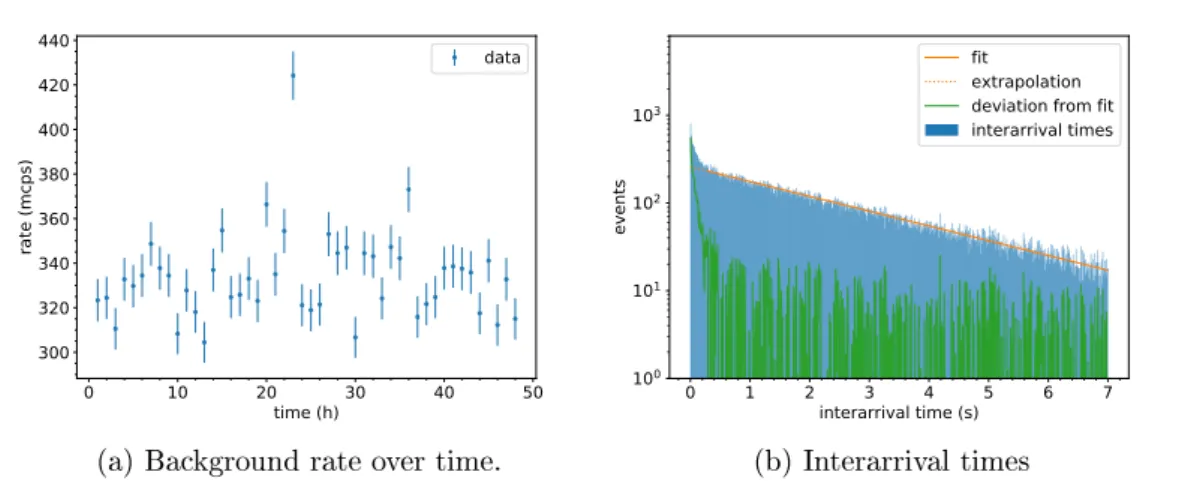
For this purpose, the pressure in the spectrometers was increased via the injection of argon to 3.0×10⁻⁹mbar [21]. Subsequently a 48 h background measurement with a closed valve between the PS and the CPS was performed. Noisy pixels (for KNM1 given in table D.1) are excluded. This dataset will be labelled as background dataset 1 (BKG1) for future reference.

(31)

4.2. EXPERIMENTAL INPUT 21

As the rate during this measurement shows no drifts (see g. 4.2a), the data can be used for ensuing analysis. The interarrival times are shown in g. 4.2b. The expected deviation from a exponential distribution is visible for small interarrival times. This motivates the denition of a limit t_NP = 0.3 s indicating the existence of a NP background component. Therefore interarrival times less thant_NP are excluded from the exponential t in g. 4.2b.

0 10 20 30 40 50

time (h) 300

320 340 360 380 400 420 440

rate (mcps)

data

(a) Background rate over time.

0 1 2 3 4 5 6 7

interarrival time (s) 10⁰

10¹ 10² 10³

events

fitextrapolation deviation from fit interarrival times

(b) Interarrival times

Figure 4.2: (a) Background rate over time of BKG1 using a 1 h time binning. The errors shown are from a Poisson expectation. (b) Interarrival times of BKG1. A deviation from the exponential t can be seen at short interarrival times. Interarrival times larger than7 s are neglected.

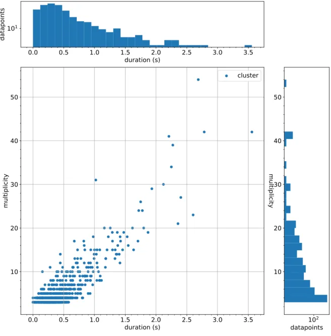
Furthermore a simple clustering can be applied. Events with an interarrial time less than t_NP are grouped in one cluster, as sketched in g. 4.3. After this clustering, the events in one cluster (its multiplicity) represent the number of secondary electrons of a nuclear decay.

The time between the rst and the last event (the cluster duration) thus gives an estimate of the storage time of the primary electron. As from a Poisson distribution alone interarrival times less than t_NP are expected, one can suppress this random coincidence by only taking clusters with at least 3 events as an input for the simulation. Applying the clustering to the data shown in g. 4.2b leads to a distribution as shown in g. 4.4. Most of the clusters have a rather small multiplicity i.e. less than 10 events. The storage time is on the order of a few seconds.

time t_NP

event clustered

Figure 4.3: Sketch of the clustering. Events with a time dierence less thant_NPform clusters.

Applying cuts on the multiplicity of those clusters suppresses random coincidence.

As the data has been taken at an elevated pressure ofp₀ = 3×10⁻⁹mbarbut the simulation should be performed at usual conditions with a low pressure p = 1×10⁻¹¹mbar, a simple scaling is applied: