Research Collection
Journal Article
The Use of Hydrotropic Solutions for Counter-Current Separations
Author(s):
Winistorfer, Peggy; Kováts, E. Sz.
Publication Date:
1967
Permanent Link:
https://doi.org/10.3929/ethz-b-000422791
Originally published in:
Journal of Chromatographic Science 5(7), http://doi.org/10.1093/chromsci/5.7.362
Rights / License:
In Copyright - Non-Commercial Use Permitted
This page was generated automatically upon download from the ETH Zurich Research Collection. For more information please consult the Terms of use.
ETH Library
The Use of Hydrotropic Solutions for Counter-Current Separations
by Peggy Winistorfer and E. sz. Kováts, Swiss Federal Institute of Technology, Department of Industrial and Engineering Chemistry, Zurich, Switzerland
The selective dissolving proper- ties of aqueous solutions of hydro- tropically active salts* suggest their application as one of the phases in counter-current distribu- tion. However, since hydrotropic activity parallels surf ace activity (1) , such solutions emulsify on shaking with a second solvent;
therefore, their use in classical counter-current distribution has been severely limited. Recently, a new variant of an apparatus was realised (2 and 3) following the orig- inal proposal of Signer et al. (4) in which shaking the phases is avoided.
Such an apparatus has not yet been described in full detailt. In the present paper, the principle of this method will be explained together with an apparatus of our own con- struction.
A glass tube is separated into cells (see Figure 1) by the inser- tion of Teflon disks pierced by a small hole through the center. The more dense solvent which serves as the stationary phase is filled into the cells, its fmal level being lower than the central hole. The less dense solvent is pumped continuously into the first cel!, filling it up to the cen- tra! hole (the direction of flow is indicated by an arrow in Figure 1) , and then passes through the hole to the second cell, to the third cel!,
etc. Equilibration of the two phases is effected within each cell by ro- tating the glass tube about its cen- tra! axis. This rotational movement mixes the two phases and continu- ously renews their contact surfaee, leading to equilibration tinles com- parable to those obtained by shak- ing but without causing foamirig.
The upper phase is prevented from flowing from one cell to the next without effective mixing by the in- sertion of smoothly curved stainless steel plates; these also add to the efficiency of the equilibration by longitudinal mixing. Figure 2 shows the whole assembly, the operation of which is described in detail in the experimental part. Essentially, the eluent is pumped through a series of rotating tubes which are parted into cells (in this case, 8 tubes containing 650 cells) .
For the application of solutions of hydrotropically active salts in counter-current distribution, a thor- ough knowledge of their clissolving properties against different classes of substances would be desirable. In the first treatment of hydrotropy, Neuberg (6) investigated the hy- drotropic activity of several differ- ent salts on a variety of substances by looking at the saturation con- centrations. This work only gives information about the solubility of
pure substances, thus taking the pure substance as standard state.
More recently, Rath, Rau, and Wagner (1 and 7) investigated the dissolving power of many salts but on only one substance.
We have chosen as standard state the ideal diluted solution in a pure one-component non-polar system [non-polarity is defmed as a non- polar substance being only a pure paraffin or mixture of paraffins,
C11H2n+2
(8 and 9) ]. By equilibrat- ing solutions of given substances in n-heptane with solutions of hydro- tropically active salts, the partition coefficient clearly defines the chem- ical potential of the substance in the salt-solution with respect to the standard state in n-heptane. In
*In the literature the terms "hydro- tropes" and "hydrotropic substances"
are used. The definition of a "hydro- trope" should then be: "a substance which changes the solvent pro perties of water," implying obviously all water soluble substances. We pro pose to drop these terms and to speak of the "hydrotropic activity" of a sub- stance and of "hydrotropy" for the effect.
iPrivate communication from Prof.
Dr. R. Signer: The apparatus used for separations in ref. (2) and (3) will be described in a forthcoming paper (5).
362 J. of G. C.—July, 1967
0 so Zo 10 41 or.
Figure 2. Counter-current distribution apparatus showing rotating tube assembly and feed system.
L. ic,
this way one can even examine sub- stances which are completely mis- cible with both solvents.
It has been suggested that hydro- tropic action arises mainly through interactions of polar parts of the solute with the organic ion of the salt (1 and 7). For this reason two neutral salts were selected, one hav- ing a negatively-charged organic ion — potassium - 1 - octylsulfonate , and the other having a positively- charged ion — trimethyl-l-octyl- ammoniumbromide. The organic part of each salt contains the same, non-polar octyl residue.
Figure 3 shows the logarithms of the partition coefficients K, plotted against the percentage concentra- tion (in g/100 ml) of the two salts, where K, is defined in equation 1.
K, =
cone. of the substance in heptane (g.cm-3) conc. of the substance in the salt sol. (g.cm-3)
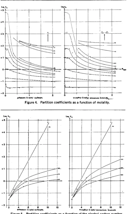
Eq. 1 The same results are shown in Fig- ure 4 but are expressed as K. against molality, where K. is defmed in equation 2
K.=
mole fraction of the substance in heptane
mole fraction of the substance in the salt sol.
simple interpretation. At low salt concentrations the partition coeffi- cients are more or less constant. For potassium-l-octylsulfonate at about 3% concentration and for trimethyl- 1-octylammonitunbromide at 4%
concentration, there is an apparent discontinuity in the shape of the curves. A hydrotropic action of the salts begins actually only at higher
concentrations. A possible explana- tion is that initially the very or- dered structure of water is broken down.
In the two figures (3 and 4) the numbered curves belong to the ho- mologuous series of primary alco- hols (2: ethanol, 3: propanol, etc., up to 12:dodecanol) . The alcohols have lower partition coefficients in
44
+3
+2
+1
—2
—3
Eq. 2 Neither presentation suggests a
0 1. Z Om.
Figure 1. Sectional view of glass coun- ter-current distribution tube showing in- dividual cells.
—
v
E--
: 's,
cl.
\•
•
'',..,....4i
C S»
S'-': '
•
7 '\
\ :
. ---....,.:_____,...s.... v A ,
,„:',„,_,._______, '---'''" ."'•.,,.._.____ n -- ---n—___L_
1. l• a
•••—•—*.--
o • --.---.__
o
k ',.,,---• . r•—• • .
10 20
+.~41,1-w-bm ~ni??
Figure 3. Partition coefficients as a function of percentage composition.
0 10 20 30 40 0
Pd0E.OrE ootionoh.
40%
cm.0
J. of G. C.—July, 1967 363
E
I \ \
\ \
•
•---, -"---.
D
1 . \
\—•
.1-..._,_.
.
C--'---•---: '„
¢lia..±.
: • - , „ , _
• :
N:,,,
•
—
.„
w...—
lo-n..._____.
•
°n..
e
3
--
•
2 po4asono-1,14,41 soSerne% 4rwor."0-1.-eoes earr000nron brown"
Figure 4. Partition coefficients as a function of molality.
Lp k.
+5
+4
+3
+2 +4
+.3
+2
+1
0
2
Plour
133—
4 6 8 10
~sloom oeWonote..
6 8 10 12
+rimr.‘041-1.-o"1 orornortiorn bron:Je.
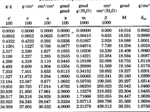
Figure 5. Partition coefficients as a function of the alcohol carbon number.
the solutions of potassium-1-octyl- sulfonate compared with those of tri- methyl -1 - octylammoniumbromide . This supports the suggestion of Rath, et al. (7) that in the case of alcohols, one of the main solubilis- ing effects is through hydrogen- bonding to the negatively-charged organic ion (in our case, of the 1- octylsulfonate ion).
Figure 5 shows the logarithms of K. plotted against the carbon-num- bers of the alcohols. This plot is linear for the distribution between heptane and pure water. However, in the case of the distribution be- tween heptane and salt solutions, the lines are curved for the lower alcohols tending to linearity for the higher members, with decreasing slope for increasing concentration of the salt.
To detect further differences be- tween the action of the two salts, four additional compounds of dis- tinctly different types were investi- gated. These are indicated by cap- ital letters in Figures 3 and 4 (A:
1-octylacetate, C: 1-chlorooctane, E: dipentylether, K: nonanone- (2) ). The results for these com- pounds are difficult to rationalise in any simple scheme. For example, the ketone (K) has a relatively low partition coefficient in both salt solutions. The ether (E) has a preferential solubility in the cati- onic solvent. Thus, simple argu- ments might suggest that the ace- tate (A) which contains both ether and ketone functions should pref- erentially dissolve in the solutions of trimethy1-1-octylammoniumbro- mide. However, the contrary is the case.
The results of the present investi- gation show that the mechanism of hydrotropic action requires much more thorough examination. How- ever, they also show that such solu- tions are capable of being used as stationary phases for counter-cur- rent distribution. The order of the elution would be non-polar sub- stances and substances of low polar- ity (hydrocarbons) , followed by more polar compounds (ethers, es- ters, aldehydes, ketones, etc.) , and fmally alcohols. In a homologous series the higher members are eluted first. Preliminary attempts to achieve separations using a solu- Von of potassium-1-octylsulfonate as stationary phase in our counter- current apparatus are promising.
Experimental
Materials
Potassium-l-octylsulfonate was
synthesised by the method of Backer (10). Octyl bromide (257 g, 1.33 mole) was heated with an aqueous solution of soclium sulfite (193 g sodium sulfite, 1.54 mole in 750 ml water) in a copper auto-
clave at 170°C for 14 hrs. To the resulting hot reaction mixture, so- dium chloride (200 g) was added.
By cooling the solution the sulfo- nate could be obtained as a wet crust. The product was freed from water by pressing in a cloth, and the air-dried product was crystal- lised from absolute ethanol.
An aqueous solution of the so- dium sulfonate was filtered onto
364 J. of G. C.—July, 1967
an ion exchange column (2000 g Dowex 50 W, 20-50 mesh, prepared as potassium salt). The resulting solution of the potassium sulfonate was evaporated to dryness and the solid product recrystallised from ethanol giving 227 g (75%) potas- sium-1-octylsulfonate as white crys- tals.
Densities of aqueous solutions of the two salts: The densities of the solutions were determined in a pyk- nometer. Tables II and III show the experimental results.
Variance analysis of the results shown in Tables II and III resulted by proving the significance of Pr, Pee, PCCC, PT, PTT, PCPT, Pel" vr
for potassium-1-octylsulfonate and Po, PT, PTT, PCPT for trimethy1-1- octylammoniumbromide at the 95%
significance level (Pe, P00, Poco sym- bolizing the linear, quadratic, cubic, etc., orthogonal polynorninals). Re- gression equations were calculated with the aid of the significant terms.
They allow the calculation of the
C H K
calc 41.35 7.38 16.83 % found 41.26 7.18 16.85 % Trimethy1-1-oetylammoniumbro- mide: Octyl bromide (485 g, 2.51 mole) was mixed with trimethyl- amine (150 g, 2.54 mole) in a pres- sure flask and was allowed to stand for 72 hrs. at room temperature.
The crude crystalline product was recrystallised from acetone giving 393 g (62%) trimethyl-l-octylam- moniumbromide (rn.p. 221/2°C) .
C H N Br
calc. 52.38 10.39 5.55 31.68 % found 52.24 10.45 5.70 31.51 % Properties of the aqueous
solutions of the two salts
Solubility of potassium-l-octyl- sulfonate: Saturated solutions of this salt were gelatinous and a quan- titative value of the saturation con- centration could not be obtained.
The solubility of the salt was cer- tainly over 47% at 00 and 22°C.
Solubility of trimethyl-1-oetylam- moniumbromide: Nearly saturated solutions of the salt in water were saturated by pressing through a thermostatted column filled with pills of the salt. Five ml. of the elu- ent was evaporated to dryness and weighed. Table I shows the satura- tion concentrations and the densi- ties at different temperatures.
Table I. Saturation concentra- tions and densities of trimethyl-l- octylammoniumbromide in water.
solubility
temp. g/100 g density ( °C) solution) (g.cm-3)
0 69.5 1.0867
5 68.7 1.0827
10 70.5 1.0827
15 70.7 1.0783
20 71.2 1.0746
concentration (g/g)
Table II. Densities of aqueous solutions of potassium-l-octylsulfonate
temperature ( °C)
0 20 40 60
0.9999 0.9982 0.9922 0.9832
15 1.0426 1.0373 1.0281 1.0179
30 1.0731 1.0652 1.0547 1.0432
45 1.1121 1.1005 1.0888 1.0760
Table III. Densities of aqueous solutions of trimethyl-l-octylammoniumbromide
concentration temperature (°C)
(g/g) 0 20 40 60
0.9999 0.9982 0.9922 0.9827
16.7 1.0199 1.0147 1.0070 0.9965
33.3 1.0405 1.0327 1.0227 1.0102
50.0 1.0606 1.0492 1.0404 1.0266
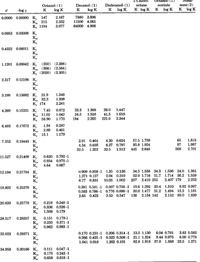
Table IV. Concentrations of the aqueous solutions used of potassium-l-octylsulfonate at 20°C
g/g g/cm3 cm3/cm3 gmol gmol cm3 gmol g/C.1113
gmol g (1-120) cm3 (I
-1,0)
c' c a P M cl,o
100 100 100 100 1000 1000
0.0000 0.0000 0.0000 0.0000 0.00000 0.000 18.016 0.9982 0.0953 0.0952 0.0635 0.0073 0.00410 0.635 18.031 0.9989 0.4322 0.4322 0.292 0.0336 0.01867 2.928 18.088 1.0001 1.1201 1.1227 0.768 0.0877 0.04874 7.739 18.204 1.0023 2.317 2.330 1.627 0.1835 0.10206 16.539 18.409 1.0060 3.199 3.227 2.285 0.2555 0.14221 23.384 18.564 1.0087 4.269 4.319 3.110 0.3445 0.19189 32.098 18.755 1.0118 6.493 6.609 4.904 0.5354 0.29880 51.569 19.164 1.0178 7.353 7.501 5.633 0.6115 0.34152 59.692 19.327 1:0201 11.527 11.872 9.284 1.0000 0.56065 102.341 20.160 1.0299 12.184 12.567 9.877 1.0632 0.59703 109.595 20.297 1.0314 19.802 20.725 17.014 1.8782 1.06250 205.023 22.042 1.0466 20.839 21.850 17.961 2.0000 1.13279 218.932 22.304 1.0485 28.517 30.216 24.928 3.0000 1.71666 332.055 24.447 1.0626 32.023 34.245 28.047 3.5234 2.02713 389.796 25.569 1.0694 34.958 37.601 30.532 4.0000 2.31278 439.512 26.591 1.0756
J. of G. C.-July, 1967 365
density between the experimental limits. The densities as a function of the linear orthogonal polynom- ials are as follows:
for potassium-1-octylsulfonate:
d =- 1.04677 + 0.02621 Po - 0.00070 P20 0.00304 1230
- 0.00899 PT - 0.00106 P2T - 0.00209 POPT
+0.00049 PoP2T
Eq. 3 where
Po = -1.5 -0.5 +0.5 +1.5
c' = 0 15 30 45
% (g/g)
PT = -1.5 -0.5 +0.5 +1.5
T= 0 20 40 60
(DC)
C (gsalt/CM3solution) C = c' • d20
Eq. 5 a (cmaal tienalsolutIon) From the density determinations the specific volume V = lid can be calculated.
The partial volume of the salt which satisfies (6)
V = C • Vsa 1 t (1 - C) VH20
Eq. 6 can easily be calculated with the aid (4 the equation 7
Vsait = V - c (aViac') Eq. 7
The volume fraction is then given by
a = C • Vaalt
Eq. 8 x (g molesalt/g molesolution): For the mixture of the components a mean molecular weight can be de- fmed which in our case is as fol- low s :
1 e,ait
4;1 -- eaatt
Mso
lution
It
wif
Eq. 9
Table V. Concentrations of the aqueous solutions used of trimethyl-l-octylammoniumbromide at 20°C
for trimethyl-l-octylammoniumbro- mide:
g/g c'
g/cm3 c
cm3/cm3 a
gmol gmol x
gmol g (11,0)
m
cm3 cm3 (H20)
P
gmol M
g/cm3
d = 1.01996 + 0.01699 Po 100 100 100 100 1000 1000 cin
- 0.00868 PT - 0.00126 P2T
- 0.00183 PoPT 0.0000 0.0000 0.0000 0.0000 0.00000 0.000 18.016 0.9982 Eq. 4 0.1034 0.1031 0.0948 0.0074 0.00410 0.949 18.033 0.9972
where 0.4692 0.4681 0.431 0.0337 0.01869 4.329 18.095 0.9976
Po = -1.5 -0.5 +0.5 +1.5 1.2158 1.2139 1.116 0.0878 0.04879 11.286 18.222 0.9984 2.515 2.514 2.306 0.1839 0.10227 23.604 18.447 0.9998 0 16.7 33.3 50.0 3.501 3.504 3.210 0.2584 0.14383 33.165 18.621 1.0009
% (g/g) 4.634 4.644 4.245 0.3458 0.19263 44.332 18.826 1.0021
6.81:il 6.831 6.223 0.5185 0.28928 66.360 19.230 1.0044 PT = -1.5 -0.5 +0.5 +1.5 7.981 8.026 7.300 0.6156 0.34383 78.749 19.458 1.0057
12.404 12.533 11.346 1.0012 0.56136 127.981 20.361 1.0104 T= 0 20 40 60 13.225 13.374 12.097 1.0768 0.60417 137.618 20.538 1.0113
(°C) 21.493 21.927 19.734 1.9178 1.08530 245.858 22.508 1.0202
22.200 22.664 20.398 1.9972 1.13120 256.245 22.694 1.0209 Concentration data 30.192 31.083 27.944 2.9964 1.71455 387.809 25.035 1.0295 34.759 35.955 32.323 3.6656 2.11208 477.607 26.602 1.0344 Knowing the density and the mo-
lecular weights, the concentration data in different dimensions can be interconverted. Table IV and V show the interconverted data for the solutions used at 20°C. They were calculated as follows:
36.799 38.146 34.331 3.9925 2.30821 522.789 27.368 1.0366
(gsait/gsolution): Solutions were prepared by weighing the salt and the water. This concentration is in-
Tabie !Va. Concentrations of the substances and markers in n
-heptane substance concentration marker concentration
(g/100 cm3801) (gmo1/1201) (g/100.01)
ethanol 4.622 1.0 hexane 0.470
dependent of temperature.
propanol- (1) 1.207 0.2 hexane 0.492
butanol- (1) 1.479 0.2 undecane 0.490
pentanol- (1) 1.770 0.2 decane 0.490
hexanol- (1) 2.040 0.2 undecane 0.488
octanol- (1) 2.603 0.2 decane 1.452
decanol- (1) 3.160 0.2 undecane 0.962
I
'dodecanol- (1) 3.720 0.2 tridecane 0.956
dipentylether 3.171 0.2 undecane 1.439
0
.1 L1-chlorooctane 2.980 0.2 undecane 1.449
Figure 6. Small stoppered glass tube 1-acetoxyoetane 3.458 0.2 dodecane 1.441
used for equilibration of n-heptane and
salt solutions. nonanone- (2) 2.852 0.2 undecane 1.448
366 J. of G. C.-July, 1967
where M's represent molecular weights. The mean molecular weight allows then calculation of the "g moles of the solution."
7Isolution = r/salt 97H20 Wsolution Msolution
Eq. 10 where w is the weight. The mean molecular weights are given in Table IV and V. Knowing the mean molecular weight, the mole fraction of the solution is given by (11)
C'
• Msoluiton Xsalt =Msalt
Eq. 11 m (g mole
sal t/cm ) : The mo-
31120-lality of the salt can be calculated as
m = Malt • c// (1 — c') Eq. 12 13 (cm' Balt' cm3H2o) : The volume ra- tio is defined by (13)
P = (cv satt) — c) • vmol
Eq. 13 and can easily be calenlated if the function a is known and is given by
p «1(1— a)
Eq. 14 Determination of the
partition coefficients
Equilibration of the two phases:
The substance to be examined was dissolved in the organic phase (n- heptane) . 1 ml of this solution of known concentration was placed in a small glass tube (Figure 6), and 1 ml of the salt solution was added together with a small nickel ball.
The tube was closed and fixed on an axis which was moving with a rocking motion with a period of 4 RPM under thermostatted water (20.0°C) . Thus, the two phases passed over each other and in ad- dition were mixed by the falling movement of the nickel bal!.
Experiments have shown that the kinetics of the substance transport from one phase to the other had a half-life of about 20 sec. For secur- ity the two phases were equilibrated for 30 min. Finally, the tube was quickly centrifuged at room tem- perature, and a small part of the heptane phase was taken for gas chromatographic analysis.
Gas chromatographic analysis:
All the substances investigated were chosen to be volatile for rapid con- centration determination by gas chromatography. In the hydrotropic solutions used, the n-paraffins were practically insoluble. Experiments with n-decane have shown that the partition coefficient of this substance is certainly higher than 1000. Thus, these substances can be used as markers, assuming their concentra- tions are unchanged during the equilibration experiment. Table IVa shows the concentration of sub- stances in n-hept,ane as well as those of the markers.
The concentration of the sub- stance was taken as low as possible with the exception of the ethanol.
In the latter case the partition co- efficients were very low, and an analysis was only possible at higher concentrations. Proof will be given that the concentration chosen can be regarded as ideal diluted.
For the evaluation of the chro- matograms a correction factor f (15) bas been determined with the aid of the prepared solutions, which allows the calculation of the con- centration of the substances from the ratio of the peak-areas (sub- stance/marker) . This is given from the chromatograms of the prepared solutions:
A, c„
Am c,
Eq. 15 where A is the peak-area in the chromatogram and c the concentra- tion in g/cm3.
After equilibration, the n-heptane phases were again chromatographed and the area-ratio determined giv- ing
ca = (A's/A'm) • cm • 1/f Eq. 16 the index a referring to the heptane phase.
The concentration cs,a would be the correct concentration for in- finitely diluted solutions. For more concentrated solutions the sub- stance transport during equilibra- tion is accompanied by a volume change, SV; i.e., the volume of the both phases after equilibration is
Vao + 8V and vp,0 — 8V. Sup-
posing that the substance dissolves in both phases without volume con-
traction, then SV is given by 8V = Va,„ • (c,,a,„ — c*,,a)
Eq. 17 where Va,„ is the volume of the heptane phase before equilibration.
The corrected concentration is then given by (18)
1 cs'a c*s'`' • 1 — (8V/Va,0)
Eq. 18 The concentration in the salt solu- tion (phase p) was in most cases not determined. It can be calcu- lated if c*a is known:
cs,p = c*S,a,„ — c*,,a) • 1
1/0 + ( 8V/Va,o)
Eq. 19 where (1) is the phase ratio (Va,„/
vp,o)
Calculation of the partition co- efficients: from the above results the partition coefficients can be cal- culated as:
K, = cs,a/cs,/3
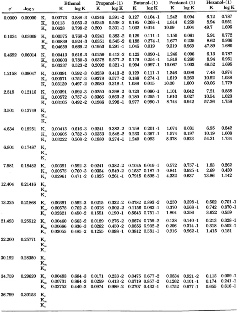
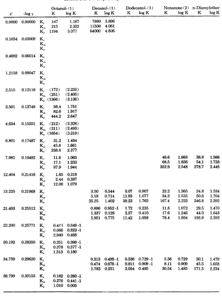
Eq. 20 Tables V and VI show the experi- mentally determined partition co- efficients, K, and their logarithms as well as two other partition co- efficients (Km and K., see below) with their logarithms, which can be calculated from K,:
a) if the concentration of the sub- stance is given in mass of substance per mass of solution, the partition coefficient Km can be calculated:
= K, • (d/3/da) = d
1t •
K
0 dheptane
Eq. 21 for the ideal diluted case.
b) if the concentration of the sub- stance is given in mole fraction or mole % the partition coefficient changes into:
d M
K.= Kc scdutton
heptanedheptane
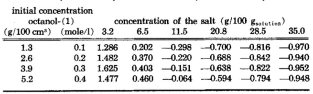
MsolutIonEq. 22 Dependence of the partition co- efficients on the substance concen- tration: Tables VII and VIII show the logarithms of the partition co- efficients K, at different salt con- centrations and with different sub- f=
d,
J. of G. C.—July, 1967 361
Table V. Partition coefficients between heptane and aqueous solutions of potassium-l-octylsulfonate
c' -log y
Ethanol K log k
Propanol- (1) K log K
Butanol- (1) K log K
Pentanol- (1) K log K
Hexanol- (1) K log K 0.0000 0.00000 K, 0.00773 0.888-3 0.0246 0.391 -2 0.127 0.104-1 1.242 0.094 6.12 0.787
Km 0.0113 0.053 -2 0.0345 0.555 -2 0.185 0.268 -1 1.814 0.259 8.94 0.951 K. 0.0628 0.798-2 0.200 0.301 -1 1.032 0.014 10.09 1.004 49.7 1.696 0.0953 0.03009 K, 0.00437 0.640 -3 0.0232 0.366-2 0.141 0.149 -1 1.288 0.110 6.77 0.831 Km 0.00639 0.805-3 0.0339 0.530-2 0.206 0.314 -1 1.881 0.275 9.90 0.996 K. 0.0355 0.550-2 0.189 0.276-1 1.145 0.059 10.46 1.020 55.5 1.744 0.4322 0.06011 K, 0.00668 0.825-3 0.0241 0.382 -2 0.129 0.111 -1 1.134 0.055 6.57 0.818 Km 0.00978 0.990-3 0.0353 0.548 -2 0.189 0.276 -1 1.659 0.220 9.61 0.983 K. 0.0542 0.734 -2 0.195 0.290-1 1.045 0.019 9.19 0.963 53.2 1.726 1.1201 0.09042 K, 0.00437 0.640-3 0.0241 0.382-2 0.135 0.131 -1 1.212 0.084 5.37 0.730 Km 0.00641 0.807 -3 0.0353 0.548-2 0.198 0.297 -1 1.776 0.250 7.87 0.896 K. 0.0353 0.548-2 0.1945 0.289-1 1.089 0.037 9.78 0.990 43.4 1.638 2.317 0.12106 K, 0.00367 0.565-3 0.0250 0.398 -2 0.136 0.134 -1 1.161 0.065 6.54 0.816 Km 0.00540 0.732-3 0.0368 0.566-2 0.200 0.301 -1 1.709 0.233 9.62 0.984 K. 0.0294 0.469 -2 0.200 0.301 -1 1.088 0.037 9.29 0.968 52.3 1.719 3.199 0.13692 K,
Km
4.269 0.15231 K, 0.00322 0.508-3 0.0232 0.366-2 0.116 0.065 -1 0.555 0.744 -1 1.968 0.294 Km 0.00477 0.679 -3 0.0343 0.535 -2 0.172 0.235 4 0.822 0.915 -1 2.91 0.464 K. 0.0255 0.406 -2 0.1834 0.263 -1 0.917 0.962 -1 4.39 0.642 15.55 1.192 6.493 0.17672 K,
Km
7.353 0.18443 K, 0.00390 0.591 -3 0.0223 0.349-2 0.0889 0.949 -2 0.272 0.435 -1 0.574 0.759-1 Km 0.00582 0.765-3 0.0333 0.522-2 0.1326 0.123 -1 0.406 0.609 -1 0.856 0.932-1 K. 0.0302 0.480-2 0.1725 0.237 -1 0.688 0.838-1 2.10 0.323 4.44 0.647 11.527 0.21409 K,
Km K.
12.184 0.21794 K, 0.00390 0.591 -3 0.0215 0.332 -2 0.0635 0.803 -2 0.1489 0.173 -1 0.275 0.439-1 Km 0.00588 0.769 -3 0.0324 0.511 -2 0.0957 0.981 -2 0.225 0.352 -1 0.415 0.618 -1 K.. 0.0290 0.463 -2 0.1600 0.204-1 0.473 0.675 -1 1.107 0.044 2.05 0.311 19.802 0.25379 K, 0.00483 0.684 -3 0.0180 0.225 -2 0.0460 0.663 -2 0.0950 0.978-2 0.140 0.147-1
Km 0.00739 0.869 -3 0.0276 0.441 -2 0.0704 0.848 -2 0.1454 0.162-1 0.214 0.331 -1 K. 0.0336 0.526 -2 0.1251 0.098-1 0.320 0.505 -1 0.661 0.820-1 0.974 0.988-1 20.839 0.25779 K,
Km Kx 28.517 0.28357 K,
32.023 0.29371 K, 0.00503 0.702 -3 0.0154 0.187 -2 0.0349 0.542 -2 0.0560 0.748-2 0.0724 0.860-2 Km 0.00787 0.896-3 0.0241 0.382 -2 0.0546 0.732 -2 0.0876 0.943 -2 0.1132 0.054-1 K. 0.0308 0.489-2 0.0944 0.975 -2 0.214 0.330-1 0.343 0.535 -1 0.444 0.647 -1 34.958 0.30166 K,
Km Kx
368 J. of G. C.-July, 1967
Table V. (Continued) Partition coefficients between heptane and aqueous solutions of potassium-l-octylsulfonate
1-Chloro- Octanol- (1) Nona- Octanol- (1) Decanol- (1) Dodecanol- (1) octane -acetate none (2)
c' -log y K log K K log K K log K K log K K log K K log K
0.0000 0.00000 K, 147 2.167 7880 3.896 Km 215 2.332 11500 4.061 K„ 1194 3.077 64000 4.806 0.0953 0.03009 K,
Km K„
0.4322 0.06011 K, Km Kx
1.1201 0.09042 K, (250) (2.398) Km (366) (2.564) Kx (2020) (3.305) 2.317 0.12106 K,
Kx
3.199 0.13692 K, 21.9 1.340 Km 32.3 1.509 Kx 174 2.241
4.269 0.15231 K, 7.45 0.872 23.3 1.368 28.0 1.447 Km 11.02 1.042 34.5 1.538 41.5 1.618 Kx 58.90 1.770 184 2.265 221.0 2.344 6.493 0.17672 K, 1.94 0.287
Kin 2.89 0.461 Kx 15.1 1.179
7.353 0.18443 K, 2.91 0.464 4.20 0.624 57.5 1.759 65 1.815
Km 4.34 0.638 6.27 0.797 85.8 1.934 97 1.987
Kx 22.5 1.352 32.5 1.512 445 2.648 503 2.701
11.527 0.21409 K, 0.620 0.792-1 Km 0.934 0.970-1 Kx 4.64 0.667
12.184 0.21794 K, 0.909 0.958-1 1.35 0.130 34.5 1.538 34.3 1.536 24.0 1.381 1.371 0.137 2.04 0.310 52.0 1.716 51.7 1.714 36.2 1.559
Kx 6.77 0.831 10.05 1.002 257 2.410 255 2.407 179 2.252
19.802 0.25379 K, 0.381 0.581 -1 0.507 0.705 -1 19.6 1.292 20.4 1.310 9.92 0.997 0.583 0.766 -1 0.776 0.890-1 30.0 1.477 31.2 1.494 15.2 1.181
Kx 2.65 0.423 3.53 0.547 136 2.134 142 2.152 69.0 1.839
20.839 0.25779 K, 0.219 0.340-1 Km 0.336 0.526-1 Kx 1.508 0.179 28.517 0.28357 K, 0.151 0.179-1
Km 0.235 0.371 -1 Kx 0.962 0.983 -1
32.023 0.29371 K, 0.170 0.231 -1 0.206 0.314 -1 13.5 1.130 6.04 0.781 3.83 0.583 0.266 0.425 -1 0.322 0.508 -1 21.1 1.324 9.44 0.975 6.00 0.778 Kx 1.041 0.018 1.262 0.101 82.8 1.918 37.0 1.568 23.5 1.371 34.958 0.30166 K, 0.111 0.047 -1
Km 0.175 0.243 -1 Kx 0.658 0.818-1
J. of G. C.-July, 1967 389
Table VI. Partition coefficients between heptane and aqueous solutions of trimethyl-l-octylammoniumbromide
c' -log y
Ethanol K log K
Propanol- (1) K log K
Butanol- (1) K log K
Pentanol- (1) K log K
Hexanol- (1) K log K 0.0000 0.00000 K, 0.00773 0.888 -3 0.0246 0.391 -2 0.127 0.104-1 1.242 0.094 6.12 0.787
Km 0.0113 0.053 -2 0.0345 0.538 -2 0.185 0.268 -1 1.814 0.259 8.94 0.951 K. 0.0628 0.798-2 0.200 0.301 -1 1.032 0.014 10.09 1.004 49.7 1.696 0.1034 0.03009 K, 0.00575 0.760-3 0.0241 0.383 -2 0.129 0.111 -1 1.150 0.061 5.91 0.772 Km 0.00839 0.9243 0.0351 0.5452 0.188 0.274 -1 1.677 0.225 8.62 0.936 K. 0.04659 0.669-2 0.1953 0.291 -1 1.045 0.019 9.319 0.969 47.89 1.680 0.4692 0.06014 K, 0.00413 0.616-3 0.0259 0.413 -2 0.123 0.090-1 1.246 0.096 6.13 0.787 Km 0.00603 0.780-3 0.0378 0.577-2 0.179 0.254-1 1.818 0.260 8.94 0.951 K. 0.03337 0.523 -2 0.2092 0.321 -1 0.994 0.997 -1 10.067 1.003 49.52 1.695 1.2158 0.09047 K, 0.00391 0.592 -3 0.0259 0.413 -2 0.129 0.111 -1 1.246 0.096 7.48 0.874 Km 0.00571 0.757-3 0.9378 0.577 -2 0.188 0.274 -1 1.819 0.260 10.92 1.038 K. 0.03139 0.497 -2 0.2080 0.318-1 1.036 0.015 10.00 1.000 60.06 1.779 2.515 0.12116 K, 0.00391 0.592-3 0.0250 0.398-2 0.123 0.090-1 1.101 0.042 7.21 0.858 Km 0.00572 0.757-3 0.0366 0.563 -2 0.180 0.255 -1 1.610 0.027 10.54 1.023 K. 0.03105 0.492 -2 0.1986 0.298-1 0.977 0.990-1 8.744 0.942 57.26 1.758 3.501 0.13749 K,
Km K„
4.634 0.15251 K, 0.00413 0.616 -3 0.0241 0.382-2 0.159 0.201 -1 1.074 0.031 6.95 0.842 Km 0.00605 0.782 -3 0.0353 0.548 -2 0.233 0.367 -1 1.574 0.197 10.19 1.008 K, 0.03222 0.508 -2 0.1880 0.274 -1 1.240 0.093 8.378 0.923 54.21 1.734 6.801 0.17487 K,
K.
7.981 0.18482 Ke 0.00391 0.592-3 0.0241 0.382 -2 0.1045 0.019 -1 0.572 0.757-1 1.83 0.262 Kl 0.00575 0.760-3 0.0354 0.549-2 0.1537 0.187 -1 0.841 0.925 -1 2.69 0.430 K, 0.02961 0.471 -2 0.1825 0.261 -1 0.7915 0.898 -1 4.332 0.637 13.86 1.142 12.404 0.21416 K,
Km K.
13.225 0.21868 K, 0.00391 0.592-3 0.0215 0.332 -2 0.0782 0.893 -2 0.250 0.398-1 0.502 0.701 -1 Km 0.00578 0.762 -3 0.0318 0.502-2 0.1156 0.063 -1 0.370 0.568-1 0.742 0.870-1 K. 0.02821 0.450-2 0.1551 0.190-1 0.5643 0.751 -1 1.804 0.256 3.622 0.559 21.493 0.25512 K, 0.00460 0.663 -2 0.0189 0.276-2 0.0574 0.759 -2 0.138 0.140-1 0.213 0.328-1
Km 0.00686 0.836-3 0.0282 0.450-2 0.0856 0.932-2 0.206 0.314-1 0.318 0.502-1 K, 0.03055 0.485 -2 0.1255 0.098 -1 0.3812 0.581 -1 0.916 0.962 -1 1.415 0.151 22.200 0.25771 K,
Km K.
30.192 0.28350 K, K.
34.759 0.29620 K, 0.00483 0.684-3 0.0171 0.233-2 0.0475 0.677 -2 0.0834 0.921 -2 0.115 0.059 -1 Km 0.00731 0.864-3 0.0259 0.413-2 0.0719 0.857 -2 0.1262 0.101-1 0.174 0.241 -1 K. 0.02752 0.440-2 0.0974 0.989 -2 0.2707 0.432-1 0.4752 0.677 -1 0.655 0.816 -1 36.799 0.30153 K,
Km K.
310 J. of G. C.-July, 1967
Table VI. (Continued) Partition coefficients between heptane and aqueous solutions of trimethyl-l-octylammoniumbromide
c' -log y
Octanol- (1) K log K
Decanol- (1) K log K
Dodecanol- (1) K log K
Nonanone (2) K log K
n-Diamylether K log K 0.0000 0.00000 K,
Km 147 215
1.167 2.332
7880 11500
3.896 4.061 K. 1194 3.077 64000 4.806 0.1034 0.03009 K,
Km 0.4692 0.06014 K,
KIII