Introduction to the SPARC Reanalysis Intercomparison Project (S-RIP) and overview of the reanalysis systems

(1)

www.atmos-chem-phys.net/17/1417/2017/

doi:10.5194/acp-17-1417-2017

Introduction to the SPARC Reanalysis Intercomparison Project (S-RIP) and overview of the reanalysis systems

Masatomo Fujiwara¹, Jonathon S. Wright², Gloria L. Manney^3,4, Lesley J. Gray^5,6, James Anstey⁷, Thomas Birner⁸, Sean Davis^9,10, Edwin P. Gerber¹¹, V. Lynn Harvey¹², Michaela I. Hegglin¹³, Cameron R. Homeyer¹⁴, John A. Knox¹⁵, Kirstin Krüger¹⁶, Alyn Lambert¹⁷, Craig S. Long¹⁸, Patrick Martineau¹⁹, Andrea Molod²⁰, Beatriz M. Monge-Sanz²¹, Michelle L. Santee¹⁷, Susann Tegtmeier²², Simon Chabrillat²³, David G. H. Tan²¹, David R. Jackson²⁴,

Saroja Polavarapu²⁵, Gilbert P. Compo^10,26, Rossana Dragani²¹, Wesley Ebisuzaki¹⁸, Yayoi Harada^27,28, Chiaki Kobayashi²⁸, Will McCarty²⁰, Kazutoshi Onogi²⁷, Steven Pawson²⁰, Adrian Simmons²¹,

Krzysztof Wargan^20,29, Jeffrey S. Whitaker²⁶, and Cheng-Zhi Zou³⁰

1Faculty of Environmental Earth Science, Hokkaido University, Sapporo, 060-0810, Japan

2Center for Earth System Science, Tsinghua University, Beijing, 100084, China

3NorthWest Research Associates, Socorro, NM 87801, USA

4Department of Physics, New Mexico Institute of Mining and Technology, Socorro, NM 87801, USA

5Atmospheric, Oceanic and Planetary Physics, University of Oxford, Oxford, OX1 3PU, UK

6NERC National Centre for Atmospheric Science (NCAS), Leeds, LS2 9JT, UK

7Canadian Centre for Climate Modelling and Analysis, Environment and Climate Change Canada, University of Victoria, Victoria, V8W 2Y2, Canada

8Department of Atmospheric Science, Colorado State University, Fort Collins, CO 80523, USA

9Earth System Research Laboratory, National Oceanic and Atmospheric Administration, Boulder, CO 80305, USA

10Cooperative Institute for Research in Environmental Sciences, University of Colorado at Boulder, Boulder, CO 80309, USA

11Courant Institute of Mathematical Sciences, New York University, New York, NY 10012, USA

12Laboratory for Atmospheric and Space Physics, University of Colorado, Boulder, CO 80303, USA

13Department of Meteorology, University of Reading, Reading, RG6 6BB, UK

14School of Meteorology, University of Oklahoma, Norman, OK 73072, USA

15Department of Geography, University of Georgia, Athens, GA 30602, USA

16Department of Geosciences, University of Oslo, 0315 Oslo, Norway

17Jet Propulsion Laboratory, California Institute of Technology, Pasadena, CA 91109, USA

18Climate Prediction Center, National Centers for Environmental Prediction, National Oceanic and Atmospheric Administration, College Park, MD 20740, USA

19Department of Atmospheric and Oceanic Sciences, University of California Los Angeles, Los Angeles, California, CA 90095, USA

20Global Modeling and Assimilation Office, Code 610.1, NASA Goddard Space Flight Center, Greenbelt, MD 20771, USA

21European Centre for Medium-Range Weather Forecasts, Shinfield Park, Reading, RG2 9AX, UK

22GEOMAR Helmholtz Centre for Ocean Research Kiel, 24105 Kiel, Germany

23Royal Belgian Institute for Space Aeronomy (BIRA-IASB), 1180 Brussels, Belgium

24Met Office, FitzRoy Road, Exeter, EX1 3PB, UK

25Climate Research Division, Environment and Climate Change Canada, Toronto, Ontario, M3H 5T4, Canada

26Physical Sciences Division, Earth System Research Laboratory, National Oceanic and Atmospheric Administration, Boulder, CO 80305, USA

27Japan Meteorological Agency, Tokyo, 100-8122, Japan

28Climate Research Department, Meteorological Research Institute, JMA, Tsukuba, 305-0052, Japan

29Science Systems and Applications Inc., Lanham, MD 20706, USA

30Center for Satellite Applications and Research, NOAA/NESDIS, College Park, MD 20740, USA

(2)

Correspondence to:Jonathon S. Wright (jswright@tsinghua.edu.cn) and Masatomo Fujiwara (fuji@ees.hokudai.ac.jp) Received: 20 July 2016 – Published in Atmos. Chem. Phys. Discuss.: 28 July 2016

Revised: 25 December 2016 – Accepted: 27 December 2016 – Published: 31 January 2017

Abstract.The climate research community uses atmospheric reanalysis data sets to understand a wide range of processes and variability in the atmosphere, yet different reanalyses may give very different results for the same diagnostics. The Stratosphere–troposphere Processes And their Role in Cli- mate (SPARC) Reanalysis Intercomparison Project (S-RIP) is a coordinated activity to compare reanalysis data sets using a variety of key diagnostics. The objectives of this project are to identify differences among reanalyses and understand their underlying causes, to provide guidance on appropriate usage of various reanalysis products in scientific studies, particularly those of relevance to SPARC, and to con- tribute to future improvements in the reanalysis products by establishing collaborative links between reanalysis centres and data users. The project focuses predominantly on differences among reanalyses, although studies that include operational analyses and studies comparing reanalyses with observations are also included when appropriate. The empha- sis is on diagnostics of the upper troposphere, stratosphere, and lower mesosphere. This paper summarizes the motiva- tion and goals of the S-RIP activity and extensively reviews key technical aspects of the reanalysis data sets that are the focus of this activity. The special issue “The SPARC Reanal- ysis Intercomparison Project (S-RIP)” in this journal serves to collect research with relevance to the S-RIP in preparation for the publication of the planned two (interim and full) S-RIP reports.

1 Introduction

An atmospheric reanalysis system consists of a global forecast model, input observations, and an assimilation scheme, which are used in combination to produce best estimates (analyses) of past atmospheric states (including temperature, wind, geopotential height, and humidity fields). The forecast model propagates information forward in time and space from previous analyses of the atmospheric state. The assimilation scheme then blends the resulting short-range forecast outputs with input observations to produce subsequent analyses of the atmospheric state, which are in turn used to ini- tialize further forecasts. Whereas operational analysis systems are continuously updated with the intention of improving numerical weather predictions, reanalysis systems are fixed throughout their lifetime. Using a fixed assimilation–

forecast model system to produce analyses of observational data previously analysed in the context of operational fore- casting (the “re” in “reanalysis”) helps to prevent the intro-

duction of artificial changes in the analysed fields (Trenberth and Olson, 1988; Bengtsson and Shukla, 1988), although artificial changes still arise from other sources (especially from changes in the quality and/or quantity of the input observational data). The first three major reanalysis efforts started in the late 1980s, conducted by NASA, ECMWF, and a joint effort between the NMC (now NCEP) and NCAR (e.g. Ed- wards, 2010). More than 10 global atmospheric reanalysis data sets are currently available worldwide. A key for all abbreviations used in this paper is provided in Appendix A.

Abbreviations representing the names of institutes, models, satellites, and other entities are in most cases only provided in the appendix; all other abbreviations are both introduced in the text and included in the appendix.

Stratosphere–troposphere Processes And their Role in Cli- mate (SPARC) is one of four core projects of the WCRP and is sponsored by the WMO, ICSU, and IOC of UNESCO.

Research themes within the SPARC mandate include atmospheric dynamics and predictability, chemistry and climate, and long-term records for understanding climate. Reanaly- sis data sets feature prominently among the tools used by the SPARC community to understand atmospheric processes and variability, to validate chemistry–climate models, and to investigate and identify climate change (e.g. SPARC, 2002, 2010; Randel et al., 2004; and references therein). However, there are known challenges for middle-atmosphere analysis and reanalysis, including (but not limited to) smaller volumes of observational data available for assimilation, increases in noise and/or biases in the available observations with height, and unique aspects of middle-atmospheric dynamics that in- fluence the behaviour of background error covariances and other facets of the data assimilation system (e.g. Swinbank and O’Neill, 1994; Swinbank and Ortland, 2003; Polavarapu et al., 2005; Rood, 2005; Polavarapu and Pulido, 2017). It has been more than 10 years since the last comprehensive intercomparison of reanalyses and related data sets in the middle atmosphere, the SPARC Intercomparison of Middle Atmo- sphere Climatologies (SPARC, 2002; Randel et al., 2004), and several new reanalyses have been released in the inter- vening years. That intercomparison and multiple subsequent studies have shown that different results may be obtained for the same diagnostic due to different technical details of the reanalysis systems, even amongst more recent reanalyses (a list of examples has been provided by Fujiwara et al., 2012; see also the contents of this special issue). The pervasive nature of these discrepancies creates a need for a new coordinated intercomparison of reanalysis data sets with respect to key diagnostics that can help to clarify the causes

(3)

of these differences. The results of this intercomparison are intended to provide guidance on the appropriate usage of reanalysis products in scientific studies, particularly those of relevance to SPARC. The reanalysis community also ben- efits from coordinated user feedback, which helps to drive improvements in the next generation of reanalysis products.

The SPARC Reanalysis Intercomparison Project (S-RIP) was initiated in 2011 to conduct a coordinated intercomparison of all major global atmospheric reanalyses (Fujiwara et al., 2012; Fujiwara and Jackson, 2013; Errera et al., 2015; see also http://s-rip.ees.hokudai.ac.jp/). The goals of the S-RIP are (1) to better understand the differences among current reanalysis products and their underlying causes; (2) to provide guidance to reanalysis data users by documenting the results of this reanalysis intercomparison; and (3) to create a communication platform between the SPARC community and the reanalysis centres that helps to facilitate future reanalysis improvements. Documentation will include both peer-reviewed papers and two S-RIP reports published as part of the SPARC report series: a full report scheduled for publication in 2018 and an electronic-only interim report to be published before- hand.

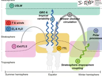
Figure 1 shows a schematic illustration of the atmosphere highlighting the processes and themes covered by the S- RIP. The planned S-RIP reports consist of two parts. Chap- ters 1–4 introduce the project, describe the reanalysis systems, and provide intercomparisons of basic variables (temperature, winds, ozone, and water vapour). These chapters will constitute the entirety of the interim report and will also be updated and included in the subsequent full report. Chap- ters 5–12 will only be included in the full report. The chapters to be included only in the full report will be arranged according to, and focus on, different regions or processes within the atmosphere, including the Brewer–Dobson circulation, stratosphere–troposphere dynamical coupling, upper- tropospheric–lower-stratospheric processes in the extratrop- ics and tropics, the quasi-biennial oscillation (QBO) and tropical variability, lower-stratospheric polar chemical pro- cessing and ozone loss, and dynamics and transport in the upper stratosphere and lower mesosphere (Fig. 1). Some important topics, such as gravity waves and transport processes, are sufficiently pervasive for related aspects to be distributed in several chapters.

The S-RIP focuses predominantly on reanalyses, although some chapters of the planned reports will include diagnostics from operational analyses when appropriate. In addition to intercomparison of the diagnostics calculated directly from reanalysis products, some chapters will include discussion of chemical transport model (CTM) and trajectory model simulations driven by different reanalysis data sets. Table 1 lists reanalysis data sets that are currently available and will be included in one or more chapters of the planned S-RIP full report. Many of the chapters focus primarily on newer reanalysis systems that assimilate upper-air measurements and produce data at a relatively high resolution (e.g. ERA-Interim,

Figure 1.Schematic illustration of the atmosphere showing the processes and regions that will be covered by chapters in the planned full S-RIP report. Domains approximate the main focus areas of each chapter and should not be interpreted as strict boundaries.

Chapters 3 and 4 cover the entire domain.

JRA-55, MERRA, MERRA-2, and CFSR/CFSv2). We also intend to include forthcoming reanalyses (e.g.ERA5) when they become available, and long-term reanalyses that assimilate only surface meteorological observations (e.g. NOAA- CIRES 20CR and ERA-20C) where appropriate. Some chapters of the planned reports will include comparisons with older reanalyses (NCEP-NCAR R1, NCEP-DOE R2, ERA- 40, and JRA-25/JCDAS) because these products have been heavily used in the past and are still being used for some studies and because such comparisons can provide insight into the potential shortcomings of past research results. Other chapters will only include a subset of these reanalysis data sets, since some reanalyses have already been shown to per- form poorly for certain diagnostics (e.g. Pawson and Fiorino, 1998; Randel et al., 2000; Manney et al., 2003, 2005; Birner et al., 2006; Monge-Sanz et al., 2007; Sakazaki et al., 2012;

Lu et al., 2015; Martineau et al., 2016) or do not extend high enough in the atmosphere. The intercomparison period com- mon to all chapters of the planned S-RIP reports is 1980–

2010. This period starts with the availability of MERRA-2 shortly after the advent of high-frequency remotely sensed data in late 1978 (the “satellite era”) and ends with the transition between CFSR and CFSv2 (see below). Some chapters will also consider the pre-satellite era before 1979 and/or include results for more recent years. Given the wide use of ERA-40 (which only extends to August 2002), separate intercomparisons for 1980–2002 are also considered for selected diagnostics.

The special issue “The SPARC Reanalysis Intercompari- son Project (S-RIP)” in this journal serves to collect research with relevance to the S-RIP in preparation for the publication of the planned two (i.e. interim and full) S-RIP reports. The

(4)

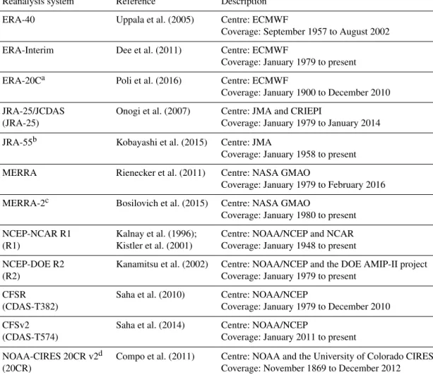
Table 1.List of global atmospheric reanalysis systems discussed in this work.

Reanalysis system Reference Description

ERA-40 Uppala et al. (2005) Centre: ECMWF

Coverage: September 1957 to August 2002

ERA-Interim Dee et al. (2011) Centre: ECMWF

Coverage: January 1979 to present

ERA-20C^a Poli et al. (2016) Centre: ECMWF

Coverage: January 1900 to December 2010 JRA-25/JCDAS Onogi et al. (2007) Centre: JMA and CRIEPI

(JRA-25) Coverage: January 1979 to January 2014

JRA-55^b Kobayashi et al. (2015) Centre: JMA

Coverage: January 1958 to present

MERRA Rienecker et al. (2011) Centre: NASA GMAO

Coverage: January 1979 to February 2016 MERRA-2^c Bosilovich et al. (2015) Centre: NASA GMAO

Coverage: January 1980 to present NCEP-NCAR R1 Kalnay et al. (1996); Centre: NOAA/NCEP and NCAR (R1) Kistler et al. (2001) Coverage: January 1948 to present

NCEP-DOE R2 Kanamitsu et al. (2002) Centre: NOAA/NCEP and the DOE AMIP-II project

(R2) Coverage: January 1979 to present

CFSR Saha et al. (2010) Centre: NOAA/NCEP

(CDAS-T382) Coverage: January 1979 to December 2010

CFSv2 Saha et al. (2014) Centre: NOAA/NCEP

(CDAS-T574) Coverage: January 2011 to present

NOAA-CIRES 20CR v2^d Compo et al. (2011) Centre: NOAA and the University of Colorado CIRES

(20CR) Coverage: November 1869 to December 2012

aA companion ensemble of AMIP simulations is also available: ERA-20CM; see Sect. 2 for details.^bTwo ancillary products are also available:

JRA-55C and JRA-55AMIP; see Sect. 2 for details.^cA companion AMIP simulation for MERRA-2 is in progress but has not yet been completed as of this writing.^dA new version of 20CR covering 1851–2011 (20CR v2c) was completed and made available in 2015.

remainder of this paper contains overview material intended to reduce duplication in subsequent papers in this special issue and is organized as follows. Section 2 is a brief introduction to the 11 global atmospheric reanalyses listed in Table 1.

Section 3 is an overview of key differences among reanalysis forecast models, with a particular focus on major physical parametrizations and boundary conditions. Section 4 is a basic description of data assimilation as implemented in current reanalysis systems. Section 5 is a summary comparison of frequently assimilated input observations, focusing on five of the most recent reanalysis systems. Section 6 includes a brief discussion of reanalysis ozone and water vapour products in the upper troposphere and stratosphere. Section 7 concludes the paper with a summary of key issues and an outline of the intended future evolution of the S-RIP activity.

2 Current reanalysis systems

In this paper, we divide reanalysis systems into three classes according to their observational inputs. “Full-input” reanalyses are systems that assimilate surface and upper-air conventional and satellite data. “Conventional-input” reanalyses are systems that assimilate surface and upper-air conventional data but do not assimilate satellite data. “Surface- input” reanalyses are systems that assimilate surface data only, with upper-air observations excluded. Some of the reanalysis centres also provide companion “AMIP-type” simulations, which do not assimilate any observational data and are constrained by applying a sea surface temperature analysis as a lower boundary condition on the atmospheric model.

The following discussion also includes the term “satellite era”, which refers to the period following 1979 (the first full year of TOVS availability), for which satellite data are relatively abundant, and the companion term “extended reanaly-

(5)

sis”, which refers to any reanalysis that provides data for the period before January 1979.

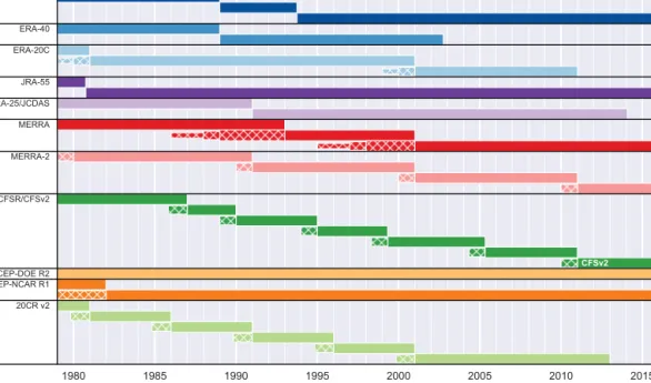
We note that the production of reanalyses must often be completed under strict deadlines. To meet these deadlines, most reanalyses have been executed in two or more distinct

“streams”, which are then combined (Fig. 2). Detailed information on stream execution is provided in the Supplement to this paper. Discontinuities in the time series of some analysed variables may occur when streams are joined. The potential impacts of these discontinuities should be considered (along with changes in assimilated observations described in Sects. 5 and 6) when reanalysis variables are used for assess- ments of climate variability and/or trends.

2.1 ECMWF reanalyses

ERA-40 (Uppala et al., 2005) is an extended full-input reanalysis covering 45 years from September 1957 through August 2002. ERA-40 was released by ECMWF in 2003 and represents an important improvement relative to the first generation of modern reanalysis systems, including FGGE (Bengtsson et al., 1982) and ERA-15 (Gibson et al., 1997). ERA-40 did not assimilate satellite data prior to Jan- uary 1973. The ERA-40 reanalysis from September 1957 through December 1972 is therefore a conventional-input reanalysis. ERA-40 products continue to be used in many studies that require long-term atmospheric data.

ERA-Interim (Dee et al., 2011), initially released by ECMWF in 2008, is a full-input reanalysis of the satellite era that includes several corrections and modifications to the system used for ERA-40. In particular, ERA-Interim uses a 4D-Var data assimilation system, which makes more com- plete use of observations collected between analysis times than the 3D-FGAT (first guess at appropriate time) approach used in ERA-40 (see Sect. 4). Major focus areas during the production of ERA-Interim included achieving more realistic representations of the hydrologic cycle and the stratospheric circulation relative to ERA-40, as well as improving the consistency of the reanalysis products in time.

ERA-20C (Poli et al., 2015, 2016) is a surface-input reanalysis produced by ECMWF and released in 2014. ERA- 20C uses a 4D-Var data assimilation system but takes its spatially and temporally varying background errors from a prior ensemble data assimilation (Isaksen et al., 2010; Poli et al., 2013). Because ERA-20C directly assimilates only surface pressure and surface wind observations, it can generate reanalyses of the climate state that extend further back in time (in this case to the beginning of the 20th century).

Assimilation of surface data indirectly constrains the upper- atmospheric state, but these constraints are relatively weak on longer-than-synoptic timescales. While data from ERA- 20C extend up to 0.01 hPa, these data should be used with caution in the upper troposphere and above. The ERA-20C model also uses sea surface temperature and sea ice concen- tration analyses as well as radiative forcings prescribed for

CMIP5. The companion product ERA-20CM (Hersbach et al., 2015) provides an ensemble of AMIP-style simulations using similar forcings and lower boundary conditions. En- semble members are spun-up from the same initial state and differ only in the prescribed evolution of sea surface temperature (SST) and sea ice, which are drawn from the HadISST2 ensemble (Titchner and Rayner, 2014; Hersbach et al., 2015).

2.2 JMA reanalyses

JRA-25 (Onogi et al., 2007), released in 2006, is a full-input reanalysis of the satellite era and the first reanalysis produced by JMA (in cooperation with CRIEPI). This reanalysis originally covered 25 years from 1979 through 2004, and was extended by an additional 10 years (through the end of January 2014) as JCDAS using an identical fixed model–

assimilation system.

JRA-55 (Kobayashi et al., 2015), released in 2013, is an extended full-input reanalysis produced by JMA. JRA-55 is the most recent reanalysis that both assimilates upper- air observations and includes coverage of the pre-TOVS era (i.e. before November 1978), starting from the International Geophysical Year (IGY) in January 1958. To date, JRA-55 is the only reanalysis system to apply a 4D-Var data assimilation scheme to upper-air data during the pre-satellite era (ERA-20C has also applied 4D-Var but only to surface observations). Two companion products are also available: JRA- 55C (Kobayashi et al., 2014), a conventional-input reanalysis, and JRA-55AMIP, an AMIP-style forecast model simulation without data assimilation. Both JRA-55C and JRA- 55AMIP were released to the public in 2015. JRA-55C is available starting from November 1972, 2 months before JRA-55 began assimilating satellite observations (before this date, JRA-55 only assimilated conventional observations so that JRA-55 and JRA-55C are identical) and extends through December 2012. JRA-55AMIP extends from January 1958 through December 2012. Extensions beyond December 2012 are planned for both JRA-55C and JRA-55AMIP, but details have not been determined as of this writing.

2.3 NASA GMAO reanalyses

MERRA (Rienecker et al., 2011), released in 2009, is a full-input reanalysis of the satellite era developed by NASA’s GMAO using the GEOS-5 data assimilation system.

MERRA was conceived with the intention of leveraging the large amounts of data produced by NASA’s Earth Observing System (EOS) satellite constellation and improving the representations of the water and energy cycles relative to earlier reanalyses. The top level used in MERRA (0.01 hPa, approximately 80 km) is higher than the top levels used in most other reanalyses, which facilitates studies extending into the mesosphere. An earlier NASA reanalysis (Schubert et al., 1993, 1995) covering 1980–1995 was produced by NASA’s DAO (now GMAO) using the GEOS-1 data assimilation sys-

(6)

1980 1985 1990 1995 2000 2005 2010 2015

20CR v2 NCEP-NCAR R1NCEP-DOE R2 CFSR/CFSv2 MERRA-2 MERRA JRA-25/JCDAS JRA-55 ERA-20C ERA-40 ERA-Interim

CFSv2

Figure 2.Summary of the execution streams of the reanalysis systems from January 1979 through December 2015. The narrowest cross- hatched sections indicate known spin-up periods, while the wider cross-hatched sections indicate overlap periods.

tem; this reanalysis is no longer publicly available and is not included in the S-RIP intercomparison.

MERRA-2 (Bosilovich et al., 2015), released in 2015, is a full-input reanalysis of the satellite era from NASA’s GMAO.

As the follow-on to MERRA, the production of MERRA-2 was motivated by the inability of the MERRA system to in- gest some recent data types. MERRA-2 includes substantial upgrades to the model (Molod et al., 2015) and changes to the data assimilation system and input data. New constraints are applied to ensure conservation of global dry-air mass and to close the balance between surface water fluxes (precipitation minus evaporation) and changes in total atmospheric water (Takacs et al., 2016). Other new features in MERRA-2 relative to MERRA include a modified gravity wave scheme that substantially improves the model representation of the QBO (Molod et al., 2015; Coy et al., 2016); the assimilation of MLS temperature retrievals at high altitudes (pressures less than or equal to 5 hPa) to better constrain the reanalysis at upper levels; the assimilation of MLS stratospheric ozone profiles and OMI column ozone since the beginning of the Aura mission in late 2004 to improve representation of fine-scale ozone features, especially in the region around the tropopause; and the assimilation of aerosol optical depth (AOD; Randles et al., 2016), with analysed aerosols fed back to the forecast model radiation scheme.

2.4 NOAA/NCEP and related reanalyses

NCEP–NCAR R1 (Kalnay et al., 1996; Kistler et al., 2001), which was first released in 1995, is the first modern reanalysis system with extended temporal coverage (1948–present)

and is produced using a modified 1995 version of the NCEP forecast model. NCEP–DOE R2 (Kanamitsu et al., 2002), released in 2000, covers the satellite era (1979–present) using a 1998 version of the same model and includes corrections for some important errors and limitations identified in R1. Both R1 and R2 remain in widespread use; however, these systems have relatively low top levels (3 hPa) and relatively coarse vertical resolutions (28 levels), and they assimilate retrieved temperatures rather than radiances from the operational nadir sounders, rendering them unsuitable for most studies of the middle atmosphere.

CFSR (Saha et al., 2010), released in 2009, is a full-input reanalysis of the satellite era that uses a 2007 version of the NCEP CFS. CFSR contains a number of improvements relative to R1 and R2 in both the forecast model and data assimilation system, including higher horizontal and vertical resolutions, a higher model top, more sophisticated model physics, and the ability to assimilate satellite radiances directly. CFSR is also the first global reanalysis of the coupled atmosphere–ocean–sea-ice system. Official data coverage by CFSR only extends through December 2009, but output from the same analysis system was continued through Decem- ber 2010 before being migrated to the operational CFSv2 analysis system (Saha et al., 2014) from January 2011. This transition from CFSR to CFSv2 should not be confused with the transfer of CFSv2 production from NCEP EMC to NCEP operations, which occurred at the start of April 2011.

CFSv2 has a different horizontal resolution and includes mi- nor changes to physical parametrizations (some of which are described below) but is intended to serve as a continuation of CFSR and can be treated as such for most purposes.

(7)

To distinguish CFSR and its CFSv2 continuation from other (mainly forecast) applications of the NCEP CFS that do not use the full data assimilation system, CFSR may also be re- ferred to as CDAS-T382 and its continuation as CDAS-T574.

NOAA–CIRES 20CR v2 (Compo et al., 2011), released in 2009, is the first reanalysis to span more than 100 years.

Like ERA-20C, 20CR is a surface-input reanalysis. Unlike ERA-20C, which uses a 4D-Var approach to assimilate both surface pressure and surface winds, 20CR uses an ensemble Kalman filter (EnKF) approach (see Sect. 4) and assimilates only surface pressure. The forecast model used in 20CR is similar in many ways to that used in CFSR, but with much coarser vertical and horizontal resolutions. 20CR provides reanalysis fields back to the mid-19th century. With only surface observations assimilated and a modest vertical resolution, 20CR is likely to be of limited utility for most studies above the tropopause and many in the upper troposphere.

3 Forecast model specifications

The forecast model is a fundamental component of any atmospheric reanalysis system. Major differences in forecast model specifications among current reanalysis systems include the horizontal grid type and spacing, the number of vertical levels, the height of the top level, the formulation of physical parametrizations, and the choice of various boundary conditions.

Table 2 provides the basic specifications for each of the reanalysis forecast models. Most of the models use spectral dynamical cores (e.g. Machenhauer, 1979), with the exception of MERRA and MERRA-2, which use finite-volume dynamics (Lin, 2004). The horizontal resolutions of the forecast models range from approximately 1.875^◦(R1, R2, and 20CR) to approximately 0.2^◦(CFSv2). A variety of notations have been used to describe Gaussian grids used in models based on spectral dynamical cores. Here, we use Fnto re- fer to the regular Gaussian grid with 2n latitude bands and (typically) 4n longitude bands. The longitude grid spacing in the standard Fn regular Gaussian grid is 90^◦/n, so that the geographical distance between neighbouring grid cells in the east–west direction shrinks toward the poles. R1, R2, and 20CR use the same regular Gaussian grid (F47), which differs from the standard in that it has 4(n+1) longitude bands and a longitude spacing of 90^◦/(n+1). JRA-25 (F80), CFSR (F288), and CFSv2 (F440) also use regular Gaussian grids. ERA-Interim, ERA-40, ERA-20C, and the JRA-55 family use linear reduced Gaussian grids (Hortal and Sim- mons, 1991; Courtier and Naughton, 1994), which are de- noted by Nn. The number of latitude bands in the Nn reduced Gaussian grid is also 2n, but the number of longi- tudes per latitude circle decreases from the equator (where it is 4n) toward the poles. Longitude grid spacing in reduced Gaussian grids is therefore quasi-regular in distance rather than degrees. The effective horizontal grid spacing is ap-

proximately 79 km for ERA-Interim (N128), approximately 125 km for ERA-40 and ERA-20C (N80), and approximately 55 km for JRA-55 (N160). Latitude bands in both regular and reduced Gaussian grids are irregularly spaced and sym- metric around the equator, with locations defined by the ze- ros of the Legendre polynomial of order 2n. The horizontal resolution of a Gaussian grid may also be described via the wavenumber truncation. Wavenumber truncations for reanalysis forecast models using regular or reduced Gaussian grids are listed in Table 2. MERRA (1/2^◦ latitude×2/3^◦ longitude) and MERRA-2 (1/2^◦ latitude×5/8^◦ longitude) use regular latitude–longitude grids.

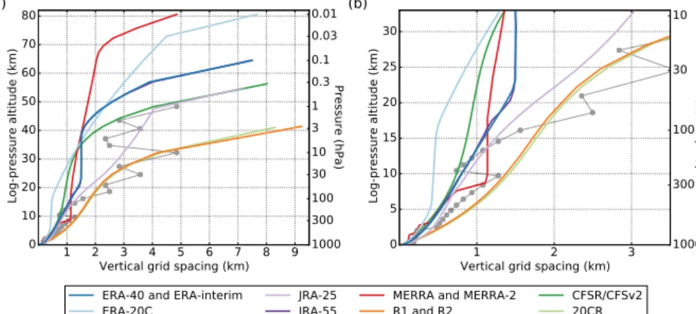
All of the reanalysis systems listed in Table 1 use hybrid σ−p vertical coordinates (Simmons and Burridge, 1981), with the exception of R1 and R2, which useσ vertical coordinates. The number of vertical levels ranges from 28 (R1, R2, and 20CR) to 91 (ERA-20C), and top levels range from 3 hPa (R1 and R2) to 0.01 hPa (MERRA, MERRA-2, and ERA-20C). Figure 3 shows approximate vertical resolutions for the reanalysis systems in log-pressure altitude, assuming a scale height of 7 km and a surface pressure of 1000 hPa. A number of key differences are evident, including large discrepancies in the height of the top level (Fig. 3a) and variations in vertical resolution through the upper troposphere and lower stratosphere (Fig. 3b). These model grids differ from the isobaric levels on which many reanalysis products are provided. Vertical spacing associated with an example set of these isobaric levels (corresponding to ERA-40 and ERA- Interim) is included in Fig. 3 for context.

In addition to differences in the location of the model top, the treatment of upper levels varies substantially across reanalysis systems. Most of the forecast models used in reanalyses implement a so-called “sponge layer”, which serves to absorb wave energy in the upper layers of the model. Sponge layers are a concession to the fact that the model atmosphere is finite, whereas the real atmosphere is unbounded at the top.

The application of enhanced diffusion in a sponge layer helps to prevent unphysical reflection of wave energy at the model top that would in turn introduce unrealistic resonance in the model atmosphere (Lindzen et al., 1968). It is worth noting, however, that diabatic heating and momentum transfer associated with the absorption of wave energy by sponge layers and other simplified representations of momentum damping (such as Rayleigh friction) may still introduce spurious behaviour in model representations of middle-atmospheric dynamics (Shepherd et al., 1996; Shepherd and Shaw, 2004).

Sponge layers in ERA-40 and ERA-Interim are implemented by including an additional function in the horizontal diffusion terms at pressures less than 10 hPa. This function, which varies with wavenumber and model level, acts as an effective absorber of vertically propagating gravity waves. The sponge layer in ERA-20C also uses this approach, along with an additional first-order diffusive mesospheric sponge layer at pressures less than 1 hPa. All three ECMWF reanalyses also apply Rayleigh friction at pressures less than 10 hPa, but the

(8)

Table 2.Basic specifications of the reanalysis forecast models. Approximate longitude grid spacing is reported in degrees for models with regular Gaussian grids (Fn) and in kilometres for models with reduced Gaussian grids (Nn). Wavenumber truncations for models with Gaussian grids are reported in parentheses.

Reanalysis system Model^∗ Horizontal grid spacing Vertical levels Top level ERA-40 IFS Cycle 23r4 (2001) N80 (TL159):∼125 km 60 (hybridσ−p) 0.1 hPa ERA-Interim IFS Cycle 31r2 (2007) N128 (T_L255):∼79 km 60 (hybridσ−p) 0.1 hPa ERA-20C IFS Cycle 38r1 (2012) N80 (T_L159):∼125 km 91 (hybridσ−p) 0.01 hPa

JRA-25 JMA GSM (2004) F80 (T106): 1.125^◦ 40 (hybridσ−p) 0.4 hPa

JRA-55 JMA GSM (2009) N160 (T_L319):∼55 km 60 (hybridσ−p) 0.1 hPa MERRA GEOS 5.0.2 (2008) 1/2^◦latitude×2/3^◦longitude 72 (hybridσ−p) 0.01 hPa MERRA-2 GEOS 5.12.4 (2015) 0.5^◦latitude×0.625^◦longitude 72 (hybridσ−p) 0.01 hPa

R1 NCEP MRF (1995) F47 (T62): 1.875^◦ 28 (σ) 3 hPa

R2 Modified MRF (1998) F47 (T62): 1.875^◦ 28 (σ) 3 hPa

CFSR (CDAS-T382) NCEP CFS (2007) F288 (T382): 0.3125^◦ 64 (hybridσ−p) ∼0.266 hPa CFSv2 (CDAS-T574) NCEP CFS (2011) F440 (T574): 0.2045^◦ 64 (hybridσ−p) ∼0.266 hPa

20CR NCEP GFS (2008) F47 (T62): 1.875^◦ 28 (hybridσ−p) ∼2.511 hPa

∗Year in parentheses indicates the year for the version of the operational analysis system that was used for the reanalysis.

1 2 3 4 5 6 7 8 9

Vertical grid spacing (km) 0

10 20 30 40 50 60 70 80

Log-pressure altitude (km)

(a)

ERA-40 and ERA-interim ERA-20C

JRA-25 JRA-55

MERRA and MERRA-2 R1 and R2

CFSR/CFSv2 20CR 1000

300 100 30 10 3 1 0.3 0.1 0.03 0.01

Pressure (hPa)

1 2 3

Vertical grid spacing (km) 0

5 10 15 20 25 30

Log-pressure altitude (km)

(b)

1000 300 100 30 10

Pressure (hPa)

Figure 3.Approximate vertical resolutions of the reanalysis forecast models for(a)the full vertical range of the reanalyses and(b) the surface to 33 km (∼10 hPa). Altitude and vertical grid spacing are estimated using log-pressure altitudes (z^∗=Hln[p₀/p]), where the surface pressurep₀is set to 1000 hPa and the scale heightHis set to 7 km. The grid spacing indicating the separation of two levels is plotted at the altitude of the upper of the two levels, so that the highest altitude shown in(a)indicates the lid location. Some reanalyses use identical vertical resolutions; these systems are listed together in the legend. Other reanalyses have very similar vertical resolutions when compared with other systems, including JRA-55 (similar but not identical to ERA-40 and ERA-Interim) and 20CR (similar but not identical to R1 and R2). Approximate vertical spacing associated with the isobaric levels on which ERA-40 and ERA-Interim reanalysis products are provided (grey discs) is shown in both panels for context.

coefficient is reduced in ERA-20C relative to ERA-40 and ERA-Interim to account for the inclusion of parametrized non-orographic gravity wave drag in ERA-20C (see also Sect. 3.1). The sponge layers in JRA-25 and JRA-55 are implemented by gradually increasing the horizontal diffusion coefficient with height at pressures less than 100 hPa. JRA-25 applies Rayleigh damping to temperature deviations from the global layer average within the top three layers of the model, while JRA-55 applies this Rayleigh damping at all pressures less than 50 hPa. MERRA and MERRA-2 increase the horizontal divergence damping coefficient in the top nine layers of the model (pressures less than∼0.24 hPa) and reduce

advection on the top level to first order. CFSR applies linear Rayleigh damping at pressures less than∼2 hPa (σ <0.002).

The horizontal diffusion coefficient also increases with scale height throughout the atmosphere in CFSR. R1, R2, and 20CR do not apply any special treatment to the model upper layers; the model tops in these systems may be thought of as lids that reflect wave energy back into the atmosphere.

Additional information on the representations of horizontal diffusion and parametrized gravity wave drag is provided in Sect. 3.1.

(9)

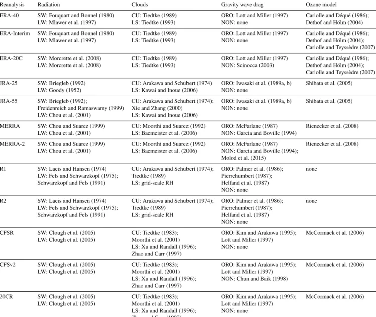
Table 3.Major physical parametrizations in the reanalysis forecast models. Radiation parametrizations are divided into shortwave (SW) and longwave (LW), cloud parametrizations are divided into convective (CU) and non-convective (LS), and gravity wave drag parametrizations are divided into orographic (ORO) and non-orographic (NON) components.

Reanalysis Radiation Clouds Gravity wave drag Ozone model

ERA-40 SW: Fouquart and Bonnel (1980) CU: Tiedtke (1989) ORO: Lott and Miller (1997) Cariolle and Déqué (1986);

LW: Mlawer et al. (1997) LS: Tiedtke (1993) NON: none Dethof and Hólm (2004)

ERA-Interim SW: Fouquart and Bonnel (1980) CU: Tiedtke (1989) ORO: Lott and Miller (1997) Cariolle and Déqué (1986);

LW: Mlawer et al. (1997) LS: Tiedtke (1993) NON: none Dethof and Hólm (2004);

Cariolle and Teyssèdre (2007) ERA-20C SW: Morcrette et al. (2008) CU: Tiedtke (1989) ORO: Lott and Miller (1997) Cariolle and Déqué (1986);

LW: Morcrette et al. (2008) LS: Tiedtke (1993) NON: Scinocca (2003) Dethof and Hólm (2004);

Cariolle and Teyssèdre (2007) JRA-25 SW: Briegleb (1992) CU: Arakawa and Schubert (1974) ORO: Iwasaki et al. (1989a, b) Shibata et al. (2005)

LW: Goody (1952) LS: Kawai and Inoue (2006) NON: none

JRA-55 SW: Briegleb (1992); CU: Arakawa and Schubert (1974); ORO: Iwasaki et al. (1989a, b) Shibata et al. (2005) Freidenreich and Ramaswamy (1999) Xie and Zhang (2000) NON: none

LW: Chou et al. (2001) LS: Kawai and Inoue (2006)

MERRA SW: Chou and Suarez (1999) CU: Moorthi and Suarez (1992) ORO: McFarlane (1987) Rienecker et al. (2008) LW: Chou et al. (2001) LS: Bacmeister et al. (2006) NON: Garcia and Boville (1994)

MERRA-2 SW: Chou and Suarez (1999) CU: Moorthi and Suarez (1992) ORO: McFarlane (1987) Rienecker et al. (2008) LW: Chou et al. (2001) LS: Bacmeister et al. (2006) NON: Garcia and Boville (1994);

Molod et al. (2015)

R1 SW: Lacis and Hansen (1974) CU: Arakawa and Schubert (1974); ORO: Palmer et al. (1986); none LW: Fels and Schwarzkopf (1975); Tiedtke (1989) Pierrehumbert (1987);

Schwarzkopf and Fels (1991) LS: grid-scale RH Helfand et al. (1987) NON: none

R2 SW: Lacis and Hansen (1974) CU: Arakawa and Schubert (1974); ORO: Palmer et al. (1986); none LW: Fels and Schwarzkopf (1975); Tiedtke (1989) Pierrehumbert (1987);

Schwarzkopf and Fels (1991) LS: grid-scale RH Helfand et al. (1987) NON: none

CFSR SW: Clough et al. (2005) CU: Tiedtke (1983); ORO: Kim and Arakawa (1995); McCormack et al. (2006) LW: Clough et al. (2005) Moorthi et al. (2001) Lott and Miller (1997)

LS: Xu and Randall (1996); NON: none Zhao and Carr (1997)

CFSv2 SW: Clough et al. (2005) CU: Tiedtke (1983); ORO: Kim and Arakawa (1995); McCormack et al. (2006) LW: Clough et al. (2005) Moorthi et al. (2001) Lott and Miller (1997)

LS: Xu and Randall (1996); NON: Chun and Baik (1998) Zhao and Carr (1997)

20CR SW: Clough et al. (2005) CU: Tiedtke (1983); ORO: Kim and Arakawa (1995); McCormack et al. (2006) LW: Clough et al. (2005) Moorthi et al. (2001) Lott and Miller (1997)

LS: Xu and Randall (1996); NON: none Zhao and Carr (1997)

3.1 Selected physical parametrizations

Table 3 provides references for some of the physical parametrizations used in the forecast models. Many of the families of models use similar parametrizations across gen- erations, but these are often modified and updated for use in newer systems. For example, both ERA-40 and ERA-Interim use shortwave radiation schemes based on Fouquart and Bon- nel (1980) and calculate longwave radiative transfer using the RRTM (Mlawer et al., 1997), but ERA-Interim uses an updated version of the shortwave scheme and makes hourly radiation calculations rather than 3-hourly ones (Dee et al., 2011). ERA-20C replaces the Fouquart and Bonnel (1980) shortwave scheme with a modified version of the RRTM

(Morcrette et al., 2008) and is the first ECMWF reanalysis to use the Monte Carlo Independent Column Approx- imation (McICA) for representing the radiative effects of clouds. Both JRA-25 and JRA-55 use shortwave radiative transfer schemes based on Briegleb (1992), but JRA-55 uses an updated parametrization of shortwave absorption by O₂, O₃, and CO₂(Freidenreich and Ramaswamy, 1999). JRA-55 also uses an updated longwave radiation model (Chou et al., 2001), which replaces the line absorption model used in JRA- 25 (Goody, 1952). R1 and R2 use identical longwave radiation schemes (Fels and Schwartzkopf, 1975; Schwartzkopf and Fels, 1991), but R1 performs radiation calculations 3- hourly on a coarser linear grid, while R2 performs radiation calculations hourly on the full model grid. R2 also uses a

(10)

different shortwave scheme (Chou and Lee, 1996) from that used in R1 (Lacis and Hansen, 1974). Both the longwave and shortwave schemes have been replaced by a modified version of the RRTMG (Clough et al., 2005) in CFSR/CFSv2 and 20CR. The McICA approach for representing cloud radiative effects has been implemented in CFSv2 but has not been used in CFSR or 20CR. MERRA and MERRA-2 both use the CLIRAD shortwave and longwave radiation schemes (Chou and Suarez, 1999; Chou et al., 2001).

Cloud parametrizations in the ECMWF family of reanalyses follow Tiedtke (1989) for convective clouds and Tiedtke (1993) for non-convective clouds, but with substantial differences among the three reanalyses. For example, modifications to the convective parametrization between ERA-40 and ERA-Interim yielded improvements in the diur- nal cycle of convection, increases in precipitation efficiency, and the capability to distinguish shallow, mid-level, and deep convective clouds (Dee et al., 2011). ERA-Interim modified the non-convective cloud parametrization to include super- saturation with respect to ice (Tompkins et al., 2007), resulting in substantial changes in the water budget of the upper troposphere. This scheme has been further modified for ERA-20C to permit separate estimates of liquid and ice water in non-convective clouds, resulting in a more physically realistic representation of mixed-phase clouds. JRA-25 and JRA- 55 both use variations of the same prognostic mass-flux type Arakawa–Schubert convection scheme (Arakawa and Schu- bert, 1974), but JRA-55 implements a new triggering mecha- nism (Xie and Zhang, 2000). MERRA-2 uses the same cloud schemes as MERRA (Table 3) but has a new set of total-water probability density functions as proposed by Molod (2012).

The representation of deep convection in R1, R2, CFSR and 20CR follows Arakawa and Schubert (1974), while the representation of shallow convection follows Tiedtke (1983). The versions of these parametrizations used in CFSR and 20CR have been updated relative to those used in R1 and R2, including the addition of convective momentum mixing to the deep-convection scheme and modifications to the shallow- convection scheme that improve the representation of marine stratocumulus (Moorthi et al., 2010; Saha et al., 2010). R1 and R2 both use simple empirical relationships to diagnose non-convective cloud cover from grid-scale relative humidity, but these relationships are slightly different between the two systems. CFSR and 20CR replace these empirical relationships with a simple cloud physics parametrization with prognostic cloud condensate (Xu and Randall, 1996; Zhao and Carr, 1997).

Gravity wave drag and ozone parametrizations are of particular interest to the SPARC community. For example, the details of the parametrization of gravity wave drag (and particularly non-orographic gravity wave drag) can greatly in- fluence the simulation of the QBO. All of the reanalysis systems include representations of orographic gravity wave sources and drag, but only MERRA, MERRA-2, CFSv2, and ERA-20C include parametrizations of non-orographic grav-

ity wave drag. MERRA-2 uses a modified version of the gravity wave drag schemes used in MERRA (McFarlane, 1987; Garcia and Boville, 1994), with enhanced intermit- tency and a larger non-orographic gravity wave background source in the tropics (Molod et al., 2015). The GEOS-5 forecast model does not produce a QBO before these changes are implemented but does produce a QBO afterwards. Start- ing with the September 2009 version (Cycle 35r3), the ECMWF IFS includes the non-orographic gravity wave drag parametrization proposed by Scinocca (2003). The version of the IFS model used for ERA-20C (the first ECMWF reanalysis to include this parametrization) produces a QBO (Hers- bach et al., 2015), but with a shorter period than observed and a weak semi-annual oscillation (SAO). CFSv2 includes a non-orographic gravity wave parametrization that consid- ers stationary gravity waves generated by deep convection (Chun and Baik, 1998; Saha et al., 2014); this parametrization was not included in CFSR. Despite the inclusion of this parametrization, the CFSv2 forecast model does not produce a QBO. The ozone parametrizations used in current reanalysis systems are introduced and discussed in Sect. 6.1.

Forecast model representations of horizontal and vertical diffusion have strong influences on tracer transport and ther- modynamic structure, particularly near the tropopause (Flan- naghan and Fueglistaler, 2011, 2014). All of the models using spectral dynamical cores include implicit linear horizontal diffusion. These implicit representations are second order (R1, R2, and 20CR), fourth order (ERA-40, ERA-Interim, ERA-20C, JRA-25, and JRA-55), or eighth order (CFSR) in spectral space. Horizontal diffusion along model sigma layers in R1 causes the occurrence of spurious “spectral precipitation”, particularly in mountainous areas at high latitudes (Kanamitsu et al., 2002). A special precipitation product was produced for R1 to address this issue, which is greatly reduced in R2. The finite-volume dynamical cores used for MERRA and MERRA-2 do not include implicit diffusion, so an explicit formulation is required. Both MERRA and MERRA-2 include explicit second-order horizontal divergence damping with a dimensionless coefficient of 0.0075 below the sponge layer. MERRA-2 also includes a second- order Smagorinsky divergence damping with a dimensionless coefficient of 0.2 that was not applied in MERRA.

The approaches to horizontal diffusion used in reanalysis schemes have been discussed in detail by Jablonowski and Williamson (2011). Approaches to vertical diffusion in the free atmosphere (above the boundary layer) are all based on the local Richardson number. ERA-40, ERA-Interim, and ERA-20C use the revised Louis scheme (Louis, 1979; Bel- jaars, 1995; Flannaghan and Fueglistaler, 2011), while JRA- 25 and JRA-55 use the level-2 turbulence closure proposed by Mellor and Yamada (1974). R1, R2, CFSR, and 20CR use the localKclosure proposed by Louis et al. (1982) in the free troposphere, but with different specifications of the background diffusion coefficients. Background diffusion coefficients in R1 and R2 are uniform throughout the atmosphere,

(11)

which results in very strong vertical mixing across the tropical tropopause (Wright and Fueglistaler, 2013). By contrast, background diffusion coefficients in CFSR and 20CR decay exponentially with height from a surface value of 1 m²s⁻¹ (Saha et al., 2010). Free-tropospheric vertical diffusion in MERRA and MERRA-2 is also parametrized based on the Louis et al. (1982) scheme, with diffusion coefficients based on the gradient Richardson number; however, a tuning pa- rameter applied in MERRA severely suppressed turbulent mixing at pressures less than∼900 hPa. That restriction has been removed in MERRA-2, but diffusion coefficients are still usually quite small in the free atmosphere. Parametriza- tions of vertical diffusion within the boundary layer vary more widely amongst reanalysis systems. These parametrizations are documented in Chapter 2 of the planned S-RIP reports, but we do not discuss them here.

3.2 Boundary conditions

Boundary and other specified conditions may be regarded as

“externally supplied forcings” to the forecast model. These conditions include all elements of the reanalysis system that are not taken from the forecast model or data assimilation but are used to produce the outputs. The factors that can be considered “external” vary somewhat among reanalyses because the forecast and assimilation components have provided a progressively larger fraction of the inputs for the forecast model as reanalysis systems have increased in sophistication.

For example, while most of the reanalyses are run with specified SSTs and sea ice concentrations, CFSR and CFSv2 are coupled atmosphere–ocean–sea-ice reanalysis systems. SST and sea ice lower boundary conditions for the CFSR and CFSv2 atmospheric models are therefore generated by coupled ocean and sea ice models (although temperatures at the atmosphere–ocean interface are relaxed every 6 hours to separate SST analyses like those used by other reanalysis systems; Saha et al., 2010). Table 4 lists the SST and sea ice analyses used by the reanalysis systems. Several reanalyses use different SSTs and sea ice concentrations for different time periods, which can lead to temporal discontinuities in reanalysis products (e.g. Simmons et al., 2010). Bosilovich et al. (2015; their Sect. 8a) further discuss these discontinuities and the steps taken in MERRA-2 to limit them and provide a cursory graphical intercomparison of the SST fields used in the production of several recent reanalyses. Ozone is another prime example of a quantity that may either be in- ternally generated or externally imposed, with particular relevance to SPARC studies. The treatment of ozone in these reanalysis systems is discussed in Sect. 6.1.

The treatment of aerosols and other trace gases also differs: MERRA-2 assimilates aerosol optical depths and uses these analysed aerosol fields for radiation calculations (Ran- dles et al., 2016), while most other systems use climatological aerosol fields. Different aerosol climatologies are used in ERA-40 (Tanré et al., 1984), ERA-Interim (Tegen et al.,

1997), JRA-25 and JRA-55 (WMO, 1986), MERRA (Co- larco et al., 2010), and CFSR and 20CR (Koepke et al., 1997). ERA-20C uses decadally varying monthly aerosol fields prepared for CMIP5 (Lamarque et al., 2010; van Vu- uren et al., 2011; Hersbach et al., 2015), while R1 and R2 neglect the role of aerosols altogether. Of the systems using prescribed aerosol fields, only CFSR, 20CR, and ERA-20C adjust them to account for the effects of volcanic eruptions.

Therefore, in the majority of reanalyses, the volcanic re- sponse in many dynamical and chemical variables is entirely due to the influences of assimilated observations. MERRA- 2 aerosol analyses, which are produced using the GOCART model (Chin et al., 2002) and the Goddard Aerosol Assim- ilation System (Buchard et al., 2015; Randles et al., 2016), track the evolution of black and organic carbon, dust, sea salt, and sulfates. These analyses are supported by the assimilation of bias-corrected AOD at 550 nm from a variety of remote-sensing platforms, including AVHRR (1980–

2000), MODIS instruments on the Terra (2000–present) and Aqua (2002–present) satellites, MISR over bright sur- faces (2000–2014), and the ground-based AERONET (1999–

2014). Analysed aerosols, including volcanic aerosols, inter- act with the MERRA-2 meteorological state via direct radiative coupling.

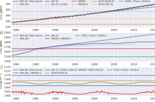
The assumptions governing greenhouse gas concentrations also vary widely. For example, the treatment of CO₂ ranges from assumptions of constant global mean CO2

(330 ppmv in R1; 350 ppmv in R2; 375 ppmv in JRA-25) to a linear trend extrapolated from observed 1990 values (ERA- 40 and ERA-Interim) to various permutations of historical observations and future emissions scenarios (all other systems). Climatological values of several other trace gases, including CH₄, N₂O, major chlorofluorocarbons (CFCs), and occasionally hydrochlorofluorocarbons (HCFCs), are used in most of the reanalysis systems but are not included in R1, R2, and JRA-25. Radiatively active trace gases (including CO₂) are generally assumed to be globally well-mixed within the atmosphere, with a few notable exceptions. First, ERA- 20C applies a rescaling to CMIP5 recommended values that varies by latitude, height, month, and species (see Hersbach et al., 2015, for details). Second, distributions of CH₄, N₂O, CFCs, and HCFCs used in MERRA and MERRA-2 are based on steady-state monthly mean climatologies generated using a two-dimensional chemistry transport model; these climatologies vary by latitude, height, and month, but trace gas concentrations do not change from year to year. Third, CFSR and 20CR (after 1955) use monthly 15^◦×15^◦gridded estimates of CO₂derived from historical WMO Global Atmo- spheric Watch observations. Figure 4a and b show temporal variations in prescribed values of CO₂ and CH₄. For sim- plicity, the base values of CO₂and CH₄ (before rescaling) are shown for ERA-20C, while values of CH₄for MERRA and MERRA-2 have been calculated using a mass- and area- weighted integral between 1000 and 288 hPa (seasonal variability in tropospheric methane is small in this climatology

(12)

Table 4.Sources of SST and sea ice lower boundary conditions used in reanalyses.

Reanalysis system Data set Grid Time Reference

ERA-40 HadISST1 (Sep 1957–Nov 1981) 1^◦ monthly Rayner et al. (2003)

NCEP 2DVar (Dec 1981–Jun 2001) 1^◦ weekly Reynolds et al. (2002) NOAA OISSTv2 (Jul 2001–Aug 2002) 0.25^◦ daily Reynolds et al. (2007)

ERA-Interim HadISST1 (Sep 1957–Nov 1981) 1^◦ monthly Rayner et al. (2003)

NCEP 2DVar (Dec 1981–Jun 2001) 1^◦ weekly Reynolds et al. (2002)

NOAA OISSTv2 (Jul 2001–Dec 2001) 0.25^◦ daily Reynolds et al. (2007)

NCEP RTG (Jan 2002–Jan 2009) 0.083^◦ daily Gemmill et al. (2007)

OSTIA (Feb 2009–present) 0.05^◦ daily Donlon et al. (2012)

ERA-20C HadISSTv2.1.0.0 0.25^◦ daily Titchner and Rayner (2014)

JRA-25/JCDAS COBE 1^◦ daily Ishii et al. (2005)

NH sea ice analysis Walsh and Chapman (2001)

SH sea ice analysis Matsumoto et al. (2006)

JRA-55^a COBE 1^◦ daily Ishii et al. (2005)

NH sea ice analysis Walsh and Chapman (2001)

SH sea ice analysis (after Oct 1978) Matsumoto et al. (2006)

MERRA Hadley Centre (Jan 1979–Dec 1981) 1^◦ monthly none (personal communication)

NOAA OISSTv2 (Jan 1982–present) 1^◦ weekly Reynolds et al. (2002)

MERRA-2 AMIP-II (Jan 1980–Dec 1981) 1^◦ monthly Taylor et al. (2000)

NOAA OISSTv2 (Jan 1982–Mar 2006) 0.25^◦ daily Reynolds et al. (2007)

OSTIA (Apr 2006–present) 0.05^◦ daily Donlon et al. (2012)

NCEP-NCAR R1 SSTs:

Met Office GISST (Jan 1948–Oct 1981) 1^◦ monthly Parker et al. (1995) NOAA OISSTv1 (Nov 1981–Dec 1994) 1^◦ weekly Reynolds and Smith (1994) NOAA OISSTv1 (Jan 1995–present) 1^◦ daily Reynolds and Smith (1994) Sea ice:

Navy/NOAA JIC (Jan 1948–Oct 1978) varies varies Kniskern (1991) SMMR and SSM/I (Nov 1978–present) 25 km monthly Grumbine (1996)

NCEP-DOE R2 AMIP-II (Jan 1979–15 Aug 1999) 1^◦ monthly Taylor et al. (2000)

NOAA OISSTv1 (16 Aug 1999–Dec 1999) 1^◦ monthly Reynolds and Smith (1994) NOAA OISSTv1 (Jan 2000–present) 1^◦ daily Reynolds and Smith (1994)

CFSR/CFSv2^a HadISST1.1 (Jan 1979–Oct 1981) 1^◦ monthly Rayner et al. (2003)

NOAA OISSTv2 (Nov 1981–present) 0.25^◦ daily Reynolds et al. (2007)

NOAA-CIRES 20CR v2^b HadISST1.1 1^◦ monthly Rayner et al. (2003)

aA climatology is used for sea ice in the Southern Hemisphere in JRA-55 prior to October 1978 (Kobayashi et al., 2015).^bCFSR and CFSv2 produce SST analyses but relax these internal products to the external SST analyses listed here (Saha et al., 2010).^cSea ice concentrations were mis-specified in coastal regions during the production of 20CR (Compo et al., 2011).

and is therefore omitted in the integrated estimate shown in Fig. 4b). The temporal evolution of greenhouse gas concentrations prescribed in these reanalysis systems is provided in the Supplement to this paper.

The representation of solar radiation at the top of the atmosphere (TOA) also varies by reanalysis. Most reanalyses assume a constant total solar irradiance (TSI) of 1365 W m⁻² (R2, JRA-25, JRA-55, and MERRA), 1367.4 W m⁻² (R1), or 1370 W m⁻²(ERA-40 and ERA-Interim). These reanalyses therefore do not explicitly account for the ∼11-year solar cycle in the radiative calculations, although the influences of this cycle may be introduced into the reanalysis via the assimilated observations (or in some cases via boundary conditions; see also Simmons et al., 2014). MERRA-2 and ERA-20C use TSI variations provided for CMIP5 historical simulations by the SPARC SOLARIS working group (Lean, 2000; Wang et al., 2005), with the Total Irradiance Monitor (TIM) correction applied. These variations account

for solar cycle changes through mid-2008 and repeat the fi- nal cycle (April 1996–June 2008) thereafter, with magni- tudes ranging from 1360.2 to 1362.7 W m⁻²between 1900 and 2008 and from 1360.6 to 1362.5 W m⁻²between 1980 and 2008. CFSR and 20CR use annual average TSI variations ranging from 1365.7 to 1367.0 W m⁻² based on data prepared by Huug van den Dool (personal communication, 2006). The solar cycle before 1944 is repeated backwards for 20CR (e.g. insolation for 1943 is the same as that for 1954, that for 1942 is the same as that for 1953, and so on) and the solar cycle after 2006 is repeated forwards in a similar manner for both CFSR and 20CR. A programming error in ERA-40 and ERA-Interim artificially increased the effective TSI by about 2 W m⁻²relative to the specified value (so that the effective TSI is∼1372 W m⁻²rather than 1370 W m⁻²).

Dee et al. (2011) reported that the impact of this error is mainly expressed as a warm bias of approximately 1 K in the upper stratosphere; systematic errors in other regions are

(13)

1980 1985 1990 1995 2000 2005 2010 2015 320

340 360 380 400 420

CO2 [ppm]

(a) ERA-40 / ERA-interim

ERA-20C

JRA-55 JRA-25 / JCDAS

MERRA MERRA-2

NCEP-NCAR R1 NCEP-DOE R2

CFSR / CFSv2 / 20CRv2

1980 1985 1990 1995 2000 2005 2010 2015

1400 1500 1600 1700 1800 1900 2000

CH4 [ppb]

(b) ERA-40 / ERA-interim

ERA-20C

JRA-55 MERRA / MERRA-2

1980 1985 1990 1995 2000 2005 2010 2015

1360 1362 1364 1366 1368 1370 1372 1374

TSI [W m−2]

(c) ERA-40 / ERA-interim

ERA-20C / MERRA-2

JRA-25 / JCDAS / JRA-55 / MERRA / NCEP-DOE R2 NCEP-NCAR R1

Figure 4.Time series of boundary conditions for(a)CO₂,(b)CH₄, and(c)TSI used by the reanalysis systems from 1979 through 2015.

The CH₄climatology used in MERRA and MERRA-2 varies in both latitude and height; here, a “tropospheric mean” value is calculated as a mass- and area-weighted integral between 1000 and 288 hPa to facilitate comparison with the “well-mixed” values used by most other systems. ERA-20C also applies rescalings of annual mean values of both CO₂and CH₄that vary by latitude, height, and month; here, the base (global annual mean) values are shown. Time series of TSI neglect seasonal variations due to the ellipticity of the Earth’s orbit, as these variations are applied similarly (but not identically) across reanalysis systems. See text for further details.

negligible. Figure 4c shows temporal variations in prescribed values of TSI from 1979 through 2015. To better highlight key differences among the reanalyses, seasonal variations resulting from the eccentricity of Earth’s orbit around the sun are omitted from the figure. These seasonal variations have peak-to-peak amplitudes of∼6.8 %, approximately 1 order of magnitude larger than the maximum difference among TSI estimates shown in Fig. 4c. The temporal evolution of TSI values prescribed in these reanalysis systems is provided in the Supplement to this paper.

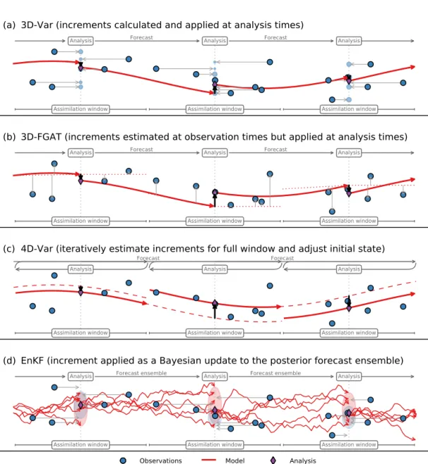
4 Data assimilation

This section provides a cursory overview of data assimilation concepts and methods as implemented in current reanalysis systems. Detailed summaries of data assimilation and its logical and mathematical foundations have been provided by Lorenc (1986), Daley (1993), Krishna- murti and Bounoua (1996), Bouttier and Courtier (1999), Kalnay (2003), Evensen (2009), and Nichols (2010), among others. As discussed above, an analysis is a best estimate of the state of a system, in this case the Earth’s atmosphere.

Data ingested into an atmospheric analysis system include observations and variables from a first-guess background state (such as a previous analysis or forecast). Both the observations and the background state include important information, and neither should be considered “truth” (as both

include errors and uncertainties). An effective analysis system reduces (on balance) the errors and uncertainties associated with both observations and the first-guess background state and therefore requires consistent and objective strategies for minimizing differences between the analysis and the (unknown) true state of the atmosphere. Such strategies often employ statistics to represent the range of potential uncertainties in the background state, observations, and techniques used to convert between model and observational space (such as spatial interpolation techniques or vertical weighting functions). Analysis systems are also generally constructed to ensure consistency with known or assumed physical proper- ties (such as smoothness, hydrostatic balance, geostrophic or gradient-flow balance, or more complex nonlinear balances).

Ensembles of analyses may be used to generate useful estimates of the uncertainties in the analysis state.

The analysis methods used by current reanalysis systems include variational methods (3D-Var and 4D-Var) and the EnKF. Variational methods (e.g. Talagrand, 2010) minimize a cost function that penalizes differences between observations and the model background state, with a consideration of associated uncertainties. Implementations of variational data assimilation may be applied to derive optimal states at dis- crete times (3D-Var) or to identify optimal state trajectories within finite time windows (4D-Var). In EnKF (e.g. Evensen, 2009), an ensemble of forecasts is used to define a probability distribution of background states (the prior distribution), which is then combined with observations (and associated