and the ERA5 Reanalysis

(1)

and the ERA5 Reanalysis

S. A. Josey¹ , M. F. de Jong², M. Oltmanns³ , G. K. Moore^4,5 , and R. A. Weller⁶

1National Oceanography Centre, Southampton, UK,²Royal Netherlands Institute for Sea Research (NIOZ) and Utrecht University, Texel, Netherlands,³GEOMAR Helmholtz Centre for Ocean Research Kiel, Kiel, Germany,

4Department of Physics, University of Toronto, Toronto, Ontario, Canada,⁵Department of Chemical and Physical Sciences, University of Toronto, Mississauga, Mississauga, Ontario, Canada,⁶Woods Hole Oceanographic Institution, Woods Hole, MA, USA

Abstract

Ground-breaking measurements from the ocean observatories initiative Irminger Sea surface mooring (60°N, 39°30⁰W) are presented that provide theﬁrst in situ characterization of multiwinter surface heat exchange at a high latitude North Atlantic site. They reveal strong variability (December 2014 net heat loss nearly 50% greater than December 2015) due primarily to variations in frequency of intense short timescale (1–3 days) forcing. Combining the observations with the new high resolution European Centre for Medium Range Weather Forecasts Reanalysis 5 (ERA5) atmospheric reanalysis, the main source of multiwinter variability is shown to be changes in the frequency of Greenland tip jets (present on 15 days in December 2014 and 3 days in December 2015) that can result in hourly mean heat loss exceeding 800 W/m². Furthermore, a new picture for atmospheric mode inﬂuence on Irminger Sea heat loss is developed whereby strongly positive North Atlantic Oscillation conditions favor increased losses only when not outweighed by the East Atlantic Pattern.

Plain Language Summary

The ocean loses heat to the atmosphere in the far northern Atlantic.

This is important as heat loss influences how much deep water is formed and the strength of the Atlantic circulation. However, the amount of heat lost is poorly known because measurements are difficult to obtain in the icy, high wind conditions of the subpolar seas. New measurements from a state-of-the-art mooring in the Irminger Sea east of Greenland are presented here. They are thefirst multiwinter measurements obtained at such high latitudes and reveal strong variability in ocean heat loss. This variability is due to changes between winters in the number of intense heat loss events. The events are caused by the mountainous Greenland terrain which focuses winds into narrow, very strong jets over the ocean. We develop a new picture which explains how changing atmospheric circulation influences the number of events and hence the ocean heat loss.

1. Introduction

The high-latitude North Atlantic is one of two main dense water formation sites in the global ocean, the other being the Antarctic coastal seas of the Southern Ocean. In the North Atlantic, formation of dense water has long been known to take place in the Labrador and Nordic Seas and was also suggested to occur in the Irminger Sea. This remained under debate (de Jong et al., 2012; Pickart et al., 2008) until recently. However, mooring and Argo proﬁlingﬂoat observations now provide unequivocal evidence for Irminger Sea deep convection (de Jong & de Steur, 2016; de Jong et al., 2018; Fröb et al., 2016) and highlight the need for better understanding of ocean-atmosphere interaction in this basin.

The key air-sea coupling processes differ significantly between the Irminger, Labrador, and Nordic Seas. The Irminger Sea is thought to be strongly influenced by small-scale (~100- to 200-km cross axis) intense atmospheric tip jets, arising from larger-scale airflow interaction with Greenland (Doyle & Shapiro, 1999; Moore

& Renfrew, 2005). The typical jet structure is a zonally oriented band of extreme winds extending eastward from the southern tip of Greenland at Cape Farewell. The properties of the jet depend upon the details of the splitting that occurs when the prevailing westerly airﬂow interacts with the mountainous barrier presented by Greenland.

Key Points:

• Irminger Sea surfaceﬂux buoy analysis providesﬁrst multiwinter observations of high-latitude North Atlantic air-sea heat exchange

• Observed net heat loss varies by nearly 50% between successive years due primarily to variations in frequency of Greenland tip jets

• Positive North Atlantic Oscillation favors increased Irminger Sea heat loss only when not dominated by stronger East Atlantic Pattern

Supporting Information:

•Supporting Information S1

•Figure S1

•Figure S2

Correspondence to:

S. A. Josey,

simon.josey@noc.ac.uk

Citation:

Josey, S. A., de Jong, M. F., Oltmanns, M., Moore, G. K., & Weller, R. A. (2019).

Extreme variability in Irminger Sea winter heat loss revealed by ocean observatories initiative mooring and the ERA5 reanalysis.Geophysical Research Letters,46, 293–302. https://doi.org/

10.1029/2018GL080956

Received 16 OCT 2018 Accepted 15 DEC 2018

Accepted article online 18 DEC 2018 Published online 11 JAN 2019

This is an open access article under the terms of the Creative Commons Attribution-NonCommercial-NoDerivs License, which permits use and distri- bution in any medium, provided the original work is properly cited, the use is non-commercial and no modiﬁca- tions or adaptations are made.

(2)

In contrast, the Labrador and Nordic Seas are primarily forced by cold air outbreaks and lack jet forcing although reverse tip jets may play some role in the northeast Labrador Sea (Moore, 2003). Further understanding has been severely limited by lack of multiyear observation-based time series of the air-sea heat exchange. The primary challenges are harsh winter atmospheric (high winds and subzero temperatures) and surface ocean (extreme wave) conditions as the Irminger Sea is one of the windiest places on Earth (Moore et al., 2008). Consequently, surface-deployed instrumentation has to endure both extreme wind/waves and ice formation. Note that the contribution of freshwaterﬂuxes to the total buoyancy forcing of the Irminger Sea is likely to be small (e.g., DuVivier et al., 2016; Schmitt et al., 1989); hence, we focus on the heat exchange in this study.

As a result, high-quality measurements in the Irminger Sea have been limited until recently to short duration (2–4 weeks) research ship observations. These have provided signiﬁcant insights in various areas, for example, atmospheric model reanalysis biases (Renfrew et al., 2002).

Additionally, a surface meteorological buoy deployed southeast of Cape Farewell from late July to early December 2004 revealed biases in satellite wind speed estimates (Moore et al., 2008). However, radiativeflux measurements were not available preventing determination of the net heat exchange. Furthermore, voluntary observing ship meteorological reports are virtually absent (Figure 1) severely limiting the accuracy of heat exchange estimates using this long-standing approach (e.g., Josey et al., 1999). Hence, until now it has not been possible to assess month-to-month air-sea heatflux variations for a significant portion of the seasonal cycle.

This lack of winter information has hindered understanding of Irminger Sea ocean-atmosphere interaction leading to uncertainty in its potential roles as a dense water formation site for the Atlantic Meridional Overturning Circulation and as a carbon sink (Fröb et al., 2016). This situation has now changed radically with the deployment (at 60°N, 39°30⁰W) of the ocean observatories initiative (OOI) Irminger Sea surfaceﬂux reference site mooring.

This mooring is the highest-latitude OOI surfaceflux site in either hemisphere (see Ogle et al., 2018 for results from the highest southern hemisphere OOI deployment at 54°S, 90°W) and has been deployed onfive occasions from 2014 to 2018 (Smith et al., 2018). Data from thefirst four deployments are used here; under extreme conditions these yielded a combined total of nearly 2 years (21 months) of observations, including early winter in three successive years, that we present and analyze. Thefifth deployment starting July 2018 is in progress and not considered here.

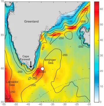
We will identify, for theﬁrst time from in situ observations, the existence of strong multiwinter variability in Irminger Sea heat loss. Furthermore, through a joint analysis of the mooring observations and the new high- resolution European Centre for Medium Range Weather Forecasts Reanalysis 5 (ERA5; Hersbach & Dee, 2016), we determine that the variability is largely driven by changes in tip jet event frequency. To set the scene, the mean and variability (calculated using individual winter means from 2000–2001 to 2017–2018) of the ERA5 winter net heatﬂux is shown in Figure 1. Strong winter to winter variability is particularly evident over the southern Irminger Sea with 2 standard deviation values of order 120 W/m²which is close to, or exceeds, half the climatological winter mean (200–250 W/m²).

Ourfindings have consequences for understanding causes of North Atlantic dense water formation variability which to date has focused on the Labrador and Nordic Seas. Our main aims are (1) to reveal thefirst in situ observation-based evidence for Irminger Sea winter heat loss variability, (2) to identify its relationship to tip jet forcing, and (3) to inform the debate on variability of drivers of North Atlantic dense water formation with reference to key atmospheric modes, in particular by suggesting a new picture for the influence of the first two modes of sea-level pressure variability on Irminger Sea heat loss.

-200

-250 -200 -200

-250

-200 -200 -100 -50

-250

Irminger Sea

Labrador Sea

SUMO Cape

Farewell Greenland

-55 -50 -45 -40 -35 -30 -25 -20

55 60 65 70

0 10 20 30 40 50 60

Figure 1.Variability of the winter net heatflux as measured by the standard deviation of the European Centre for Medium Range Weather Forecasts Reanalysis 5 December–February mean net heatflux (coloredfield, W/m²) calculated over all winters from 2000–2001 to 2017–2018. Contours indicate the climatological European Centre for Medium Range Weather Forecasts Reanalysis 5 December–February mean net heatflux over the same period.

Location of the ocean observatories initiative surfaceflux mooring (60°N, 39°30⁰W) is indicated by the white circle. Black dots show all individual voluntary observing ship reports (1 black dot = 1 report) with sufficient information to estimate the latent heatflux in an example winter month (December 2015) determined using reports in the International Comprehensive Ocean-Atmosphere Data Set (http://icoads.noaa.gov/).

(3)

2. Data Sets

The surface flux mooring (SUMO hereafter) forms part of the central Irminger Sea OOI array of four moorings, the other three having subsurface instrumentation (de Jong et al., 2018). SUMO has been deployed middle to late summer in consecutive years beginning July 2014. On each of thefirst three deployments, approximately 6 months of data were collected before the mooring sensors failed due to extreme winter conditions in January/February of the following year. On thefirst deployment, SUMO captured the winter with the most intense deep mixing observed in the Irminger Sea to date (de Jong et al., 2018).

During the fourth deployment, the mooring broke free after 3 months. Despite the environmental challenges, the resulting 21-month data set forms a unique window into Irminger Sea air-sea interaction, enabling theﬁrst accurate heat exchange characterization at timescales from hourly to more than half the annual cycle. We note that the data set provides observations for successive autumn-winter periods but as yet not spring-summer nor full seasonal cycles.

The key variables measured by SUMO are sea surface temperature, near-surface atmospheric humidity and temperature, wind speed and direction, barometric pressure, and incoming longwave/shortwave radiation.

For instrumentation and individualflux component (sensible, latent, net longwave, and net shortwave) determination details see supporting information. The net heatflux was obtained as the sum of the components with positive/negative heatflux indicating ocean heat gain/loss (e.g., Josey et al., 2013).

For ERA5, we use output covering January 2000 to April 2018. ERA5 has higher resolution (30 km) than its predecessor ERA-Interim (79 km; Dee et al., 2011) and has a revised data assimilation system and improved model physics. Index values for the North Atlantic Oscillation (NAO) and East Atlantic Pattern (EAP) modes of sea-level pressure variability have been obtained from the NOAA Climate Prediction Center.

3. Results

3.1. Daily to Multiwinter Variability

Daily mean SUMO time series of the meteorological and heatflux variables are shown in Figure 2. The expected late summer to middle winter seasonal transition is evident with falling specific humidity, air, and sea surface temperatures and increasing wind speed as the year progresses. Over the same period, the shortwave declines from values of 150–200 W/m² to close to 0, longwave ranges typically from30 to 80 W/m², and latent and sensible heat losses intensify noticeably. Considering submonthly variability, the sea surface temperature decline in each deployment is relatively smooth, but strong variations at timescales of days-weeks are apparent in the near-surface variables andflux components. Frequent daily latent (sensible) heat loss values greater than250 (150) W/m²are observed on thefirst deployment with smaller extremes in the two subsequent winters. The extremes reflect the impacts of wind speed, air temperature, and humidity variability on the latent and sensible heatfluxes. These combine primarily with the longwave (as shortwave is so small) to form net heat losses exceeding400 W/m²on at least one occasion each winter, with the strongest values exceeding600 W/m².

Another noticeable feature is the high level of variability in early to middle winter (December to early January) heat loss. The 2014–2015 net heat loss is typically stronger and has a greater frequency of intense, 1- to 3-day timescale loss events than 2015–2016 and 2016–2017, suggesting that tip jet contributions may have played a significant role (see section 3.2). Values in Table S2 show the mean component and net heat fluxes averaged over December (this month being chosen as it is common to thefirst three deployments).

The December 2014 net heat loss is241 W/m², 44% higher than December 2015 (167 W/m²) with December 2016 (205 W/m²) intermediate between the two. The drivers for this difference are lower air temperature/humidity and stronger winds, which result in December 2014 latent (sensible) heatflux mean values of120 (72) W/m², compared to72 (50) W/m²in December 2015 and87 (58) W/m²in December 2016. Also shown in Table S2 for the longer first deployment are values averaged over 1 December to 15 February (last date with available data) as a measure of winter heat loss over the nearly 3-month period sampled by the mooring in 2014–2015. These values reveal that the strong December heat loss conditions are maintained over much of the season with winter mean net heat loss of263 W/m²driven by contributions from the latent (128 W/m²), sensible (90 W/m²), and longwave (59 W/m²) heatflux components, slightly offset by a small shortwave gain (15 W/m²).

(4)

The integrated effects of the anomalously strong heat loss events in 2014–2015 are evident in Figures 2e and 2f which show cumulative time series from 1 October for each of the three winters. The 2014–2015 time series start to diverge strongly from the other two winters in early December, and by late January the 2015 integrated net heat loss is2 × 10⁹J/m²; the corresponding value for 2016 is1.4 × 10⁹J/m². The

07/14 10/14 01/15 04/15 07/15 10/15 01/16 04/16 07/16 10/16 01/17 04/17 07/17 10/17 01/18 -5

0 5 10

Temp.(o C)

a.) SST(green), 2m Air Temp.(red)

07/14 10/14 01/15 04/15 07/15 10/15 01/16 04/16 07/16 10/16 01/17 04/17 07/17 10/17 01/180 10

20 30

u10 (m s-1 )

b.) 10 m Wind Speed (black), 2m Specific Humidity (SH, green)

0 10

SH (g kg-1 )

07/14 10/14 01/15 04/15 07/15 10/15 01/16 04/16 07/16 10/16 01/17 04/17 07/17 10/17 01/18 -400

-200 0 200

Flux (W m-2 )c.) Heat Flux: Latent (blue), Sensible (green), -Longwave (magenta), Shortwave (red)

07/14 10/14 01/15 04/15 07/15 10/15 01/16 04/16 07/16 10/16 01/17 04/17 07/17 10/17 01/18 -600

-400 -200 0 200

Flux (W m-2 ) d.) Net Heat Flux

Oct Nov Dec Jan Feb Mar

-2 -1 0

Cum. Flux (J m-2 ) ₁₀⁹ e.) Cumulative Lat. & Sen. Flux

Oct Nov Dec Jan Feb Mar

-2 -1 0

Cum. Flux (J m-2 ) ₁₀⁹ f.) Cumulative Net Heat Flux

01 02 03 04 05 06 07 08 09 10 11 12 13 14 15 16 17 18 19 20 21 22 23 24 25 26 27 28 29 30 January 2015

-800 -600 -400 -200 0

Flux (W m-2 ) g.) Net Heat Flux

Figure 2.SUMO daily mean time series of (a) SST and 2-m air temperature; (b) 2-m specific humidity and 10-m wind speed, short blue vertical lines show tip jet days; (c) latent, sensible heat, net longwave (scaled by1 for clarity) and net shortwaveflux; and (d) net heatflux. (e, f) Cumulative daily mean time series beginning 1 October for 2014–2015 (solid line), 2015–2016 (dash-dotted line), and 2016–2017 (dotted line) are also shown for (e) latent and sensible heatflux and (f) net heatflux. (g) OOI hourly time series of net air-sea heatflux for January 2015. The green box in panel (d) indicates the time period shown in panel (g). SUMO = surfaceflux mooring; SST = sea surface temperature; OOI = ocean observatories initiative.

(5)

latent heat dominates with a cumulative contribution approaching twice that from sensible heat (the radiative terms, not shown, are weaker).

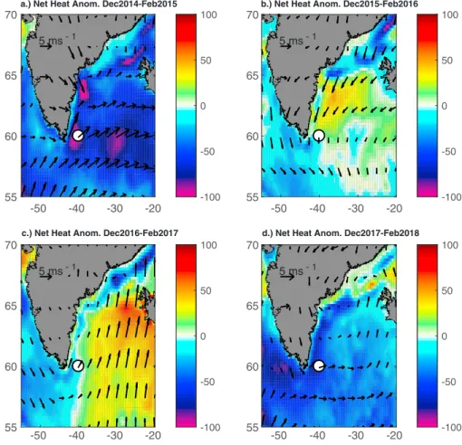
The absence of late winter data from the other deployments prevents further comparison of full winter period severity. However, we are able to explore this using ERA5 and also place the SUMO data in the context of large-scale forcing. Winter ERA5 net heatflux anomalyfields (Figure 3) are consistent with SUMO as they show that 2014–2015 winter is much more intense than 2015–2016 and 2016–2017. Furthermore, using ERA5 for all winters from 2000–2001 to 2017–2018, wefind that the correlation between the December heat flux anomaly and the anomaly for winter as a whole isr= 0.66 (0.64) for winter defined to be December– February (December–March); that is, the December heat loss may be taken to some extent as representative of the full winter.

To compare further with the mooring observations, we consider the absolute (rather than anomalous) ERA5 net heat loss values for the grid cell coincident with SUMO which are December 2014 (312 W/m²), December 2015 (217 W/m²), and December 2016 (234 W/m²). Assessment of ERA5 heatﬂux component values (not shown) indicates that the increased December 2014 heat loss is again due to a combination of latent and sensible heat losses. The ERA5 December 2014 net heat ﬂux is also 44% stronger than December 2015, that is, the same proportion as found for SUMO, indicating close agreement between the relative magnitude of successive winter heat loss variability from reanalysis and mooring (note ERA5 values are typically 50–70 W/m²greater than SUMO; the reasons for this excess will be considered in a separate reanalysis evaluation paper).

a.) Net Heat Anom. Dec2014-Feb2015

5 ms^{- 1}

-50 -40 -30 -20 55

60 65 70

-100 -50 0 50 100

b.) Net Heat Anom. Dec2015-Feb2016

5 ms^{- 1}

-50 -40 -30 -20 55

60 65 70

-100 -50 0 50 100

c.) Net Heat Anom. Dec2016-Feb2017

5 ms^{- 1}

-50 -40 -30 -20 55

60 65 70

-100 -50 0 50 100

d.) Net Heat Anom. Dec2017-Feb2018

5 ms^{- 1}

-50 -40 -30 -20 55

60 65 70

-100 -50 0 50 100

Figure 3.Winter (December, January, February) anomalous net heatﬂux (color, W/m²) from European Centre for Medium Range Weather Forecasts Reanalysis 5 for (a) 2014–2015, (b) 2015–2016, (c) 2016–2017, and (d) 2017–2018.

Anomalies are determined with respect to the 2000–2001 to 2017–2018 winter mean. Also shown are the anomalous 10-m wind speedfields for each winter (arrows). Note that heatflux values are shown on the 0.25° × 0.25° European Centre for Medium Range Weather Forecasts Reanalysis 5 grid, while wind speed is subsampled at 2.5° × 2.5°. Location of surface flux mooring indicated by the white circle.

(6)

For completeness, ERA5 anomalyﬁelds for last winter, 2017–2018, are also shown in Figure 3d. This winter has notably more intense heat loss than the preceding two and approaches the severity of 2014–2015. The 2017–2018 winter heat loss is a potential factor in the development in spring 2018 of a cold anomaly in the central subpolar North Atlantic. This anomaly may reﬂect the combined effects of the 2017–2018 winter season and reemergence of the earlier 2014–2016 cold anomaly (Duchez et al., 2016; Grist et al., 2016; Josey et al., 2018).

3.2. Relationship to Tip Jet Forcing

The 2014–2015 winter net heat loss (Figure 3a) shows enhanced loss east of Cape Farewell, consistent with the region previously identified as being influenced by tip jets (Moore, 2014; Pickart et al., 2003). This suggests that tip jet forcing plays a significant role in thefirst winter but not the following two. Averaging over a given winter may be expected to smooth out individual heat loss events potentially obscuring the contributions and spatial scales associated with tip jet forcing. The SUMO data (Figure 2d) has revealed reg- ular strong heat loss events with timescales of 1–3 days in winter 2014–2015. The strongest events occurred in January, and this is shown in detail using hourly observations (Figure 2g). Four events with heat loss exceeding400 W/m²for longer than a day are evident, with the most extreme values over800 W/m². The longest event spans 3 days from 7 to 10 January; the other three last about a day and are centered on 19–20, 22–23, and 27–28 January. In all four cases, the events are associated with intense wind speeds,

>20 m/s, that originate from the southwest (the dominant direction for tip jet generation; Moore, 2014) and enhanced latent, sensible, and longwave losses (Figure S1).

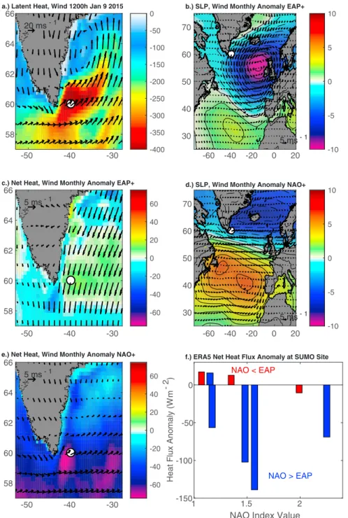
As an example, the spatial structure of the strongest component, the latent heat loss, at 1200 hr on 9 January clearly demonstrates the expected features of tip jet forcing (Figure 4a). Speciﬁcally, a region of extreme heat loss extends eastward from the tip of Greenland, in this case for about 400 km. Heat loss over the surround- ing area is much weaker indicating that the anomalous heat loss at SUMO is not the result of larger- scale forcing.

We now compare variations in frequency of tip jet conditions using SUMO data for each December sampled by theﬁrst three deployments. To do this, a tip jet criterion is applied that observed daily mean wind speeds exceed 14 m/s and wind direction is from the southwest (a similar approach was adopted for tip jet evaluation in ERA-Interim by Moore, 2014; Fröb et al., 2016). With this criterion, there are 13 days with tip jet conditions in December 2014. In contrast, December 2015 (2016) have only 2 (1) days with tip jet conditions.

Reducing the threshold value to 12 m/s increases the number of tip jet days as follows: December 2014 (15), December 2015 (3), and December 2016 (5); Figure 2b. The value that should be adopted for the threshold is not well deﬁned but it is evident that, with either choice, tip jet conditions are much more prevalent in December 2014 than in December 2015 or 2016, thus revealing the existence of strong multiwinter variability in tip jet frequency for theﬁrst time from in situ observations.

To determine typical values for the tip jet impact on net heatﬂux, the meanﬂux has been calculated for days with/without tip jet conditions for each of the three months of December using the 12-m/s threshold. The resulting values are December 2014 (299/188), December 2015 (405/141), and December 2016 (359/175 W m²); that is, the SUMO data show that tip jet conditions enhance daily mean net heat loss by 110–260 W/m². Combining these values with the frequency of events in each year, the proportion of heat loss under tip jet conditions is 60% in December 2014 compared with 24 (28)% in December 2015 (December 2016). Note that the average tip jet-related heat loss in both December 2015 and 2016 is stronger than in December 2014 as the few tip jets that did occur were characterized by conditions of particularly cold air and high sea-air temperature difference (Figure 2a).

3.3. Relationship to Atmospheric Modes of Variability

The NAO (see, e.g., Hurrell et al., 2003, for an overview of this mode) has been suggested to inﬂuence tip jet occurrence with positive NAO conditions favoring northward displacement of the winter storm track, greater interaction with Greenland, and an increase in frequency of jet conditions (Moore, 2003; Moore et al., 2011; Pickart et al., 2008). The NAO index in December 2014 (1.63) is strongly positive, supporting this suggestion given the observed prevalence of jet conditions at this time. However, in December 2015 the NAO is stronger still (1.99) but very few tip jets were observed. In December 2016, the NAO was close to neutral (0.35) consistent with the moderate number of tip jets in the mooring record.

(7)

Why did the strong NAO in December 2015 not induce more tip jets? The answer may lie with the second mode of variability, the EAP (Wallace & Gutzler, 1981). This pattern is characterized, in its negative state, by blocking in the eastern subpolar gyre that has the potential to divert the course of storms over the

d.) SLP, Wind Monthly Anomaly NAO+

5 ms^{- 1} -60 -40 -20 0 20 30

40 50 60 70

-10 -5 0 5 10 5 ms^{- 1} -60 -40 -20 0 20 30

40 50 60 70

-10 -5 0 5 10

e.) Net Heat, Wind Monthly Anomaly NAO+

5 ms^{- 1}

-50 -40 -30

58 60 62 64 66

-60 -40 -20 0 20 40 60 c.) Net Heat, Wind Monthly Anomaly EAP+

5 ms^{- 1}

-50 -40 -30

58 60 62 64 66

-60 -40 -20 0 20 40 60

f.) ERA5 Net Heat Flux Anomaly at SUMO Site

NAO > EAP NAO < EAP

1 1.5 2

-150 -100 -50 0

Heat Flux Anomaly (W m-2 ) 20 ms^{- 1}

-50 -40 -30

58 60 62 64 66

-400 -350 -300 -250 -200 -150 -100 -50 0

Figure 4.(a) ERA5 latent heat exchange (color, W/m²) and wind speed (arrows) for the 9 January 2015 extreme heat loss event at 1200 h. (b–e) Composite ERA5 net heatflux (color, W/m²), wind speed (arrows), and sea-level pressure (contours, 1-mb intervals, zero and positive solid, and negative values dashed)fields. Composites are formed by averaging over the individual December, January, and February months with the 10 most positive NAO or EAP index values in the period December 2000 to February 2018 (see Table S3 for details). (b) EAP + North Atlantic, (c) EAP + Irminger Sea, (d) NAO + North Atlantic, (e) NAO + Irminger Sea. (f) ERA5 net heatflux anomaly at the SUMO site as a function of monthly NAO index for winter months from December 2000 to February 2018 with NAO>1 and NAO>EAP (blue bars) or NAO<EAP (red bars). Location of SUMO indicated by the white circle. ERA5 = European Centre for Medium Range Weather Forecasts Reanalysis 5;

NAO = North Atlantic Oscillation; EAP = East Atlantic Pattern; SUMO = surfaceﬂux mooring.

(8)

middle- to high-latitude North Atlantic. Interactions between the NAO, the EAP, and the Scandinavian pattern (a further mode) have previously been found to impact the locations of the centers of the Iceland Low and Azores High (Moore et al., 2013). It has also been suggested that the location of the Icelandic Low modulates the frequency of tip jet events (Bakalian et al., 2007). However, the direct inﬂuence of the EAP on Irminger Sea heat loss (via tip jet suppression) has not been considered.

In December 2015, the EAP index value of 3.14 was exceptionally high. Positive EAP index values corre- spond to intense low pressure (rather than blocking), centered in the eastern subpolar North Atlantic, which may extend far enough to influence the Irminger Sea. This possibility is explored using ERA5 to determine anomalous wind, sea-level pressure, and heat flux fields under positive EAP and NAO conditions (Figures 4b–4e). The positive EAP does have a strong influence on the Irminger Sea, generating northerly flow and reduced heat loss (Figures 4b and 4c) as the sea-air temperature/humidity gradients and wind speed (not shown) are lower than normal. In contrast, as expected, the NAO is associated with westerlyflow which is noticeably perturbed at the tip of Greenland giving rise to enhanced heat loss (Figures 4d and 4e).

We now investigate whether the EAP is capable of preventing excess heat loss in the tip jet region when the NAO is strongly positive (defined here as above an index threshold of 1). The NAO>1 months were grouped according to whether the EAP index in each individual month is greater than or less than the corresponding NAO index (with the further constraint that the EAP>0 to prevent possible complications arising from a negative EAP state). The resulting heat loss at the mooring site is shown in Figure 4f where blue (red) bars indicate NAO stronger (weaker) than EAP. The influence of the EAP is clear with enhanced heat loss for NAO stronger than EAP (mean net heatflux anomaly =70 W/m²) but suppressed heat loss for NAO weaker than EAP (flux anomaly = +6 W/m²). The mechanism by which the EAP dominates the normal behavior of the NAO requires further study, but we note that previous work has shown that northerlyflow is expected to generate barrier winds that suppress tip jets (Moore & Renfrew, 2005) and this is likely a key part of the EAP influence (Figure S2). The need to consider the joint impacts of the NAO and EAP has been demonstrated in a range of studies investigating air-sea interaction in the eastern subpolar gyre (Josey &

Marsh, 2005), the centers of action of the NAO (Moore et al., 2011, 2013), and European climate (Moore

& Renfrew, 2012). Here we have shown for theﬁrst time that the EAP inﬂuence extends far enough to suppress ocean surface heat loss at the Irminger Sea dense water formation site.

To summarize this section, we have developed a revised picture for the inﬂuence of large-scale modes of variability on the frequency of tip jets whereby a positive NAO favors tip jet formation only when not dominated by stronger EAP conditions. This is important for assessment of the potential historical contribution of Irminger Sea convection to dense water formation at high latitudes in combination with the Labrador and Nordic Seas. In particular, analysis of evidence for Irminger Sea dense water formation in the sparse hydro- graphic record through the 1900s has tended to focus on the role of the NAO alone (Pickart et al., 2008), while a clearer picture may emerge if the EAP is also taken into account.

4. Conclusions and Broader Implications

This study has revealed for theﬁrst time using in situ surface mooring data the existence of strong multiwinter variability in Irminger Sea heat loss and established that it is driven by variations in the frequency of episodic heat loss at 1- to 3-day timescales. By analyzing the mooring data in combination with ERA5 reanalysis ﬁelds, the episodic heat loss has been shown to be associated with Greenland tip jet forcing of the ocean.

Furthermore, in contrast to the prevailing view that positive NAO conditions favor tip jet formation, and thus Irminger Sea deep convection, we have developed an alternative picture that recognizes the importance of the EAP. Speciﬁcally, a positive NAO only results in strong Irminger Sea heat loss when not dominated by the EAP, as the latter leads to northerlyﬂow and tip jet suppression.

Our analysis focuses on the novel OOI SUMO observations. The OOI Irminger Sea array contains a further three moorings making subsurface measurements (de Jong et al., 2018). Future work using all four moorings will enable the response of the subsurface ocean to tip jets and the potential dependence on NAO/EAP state to be explored in detail. This will beneﬁt from theﬁfth SUMO deployment that has the potential to provide data through winter 2018–2019. Additionally, we plan to use the full multidecadal period covered by ERA5 to investigate the relationship between tip jet frequency and atmospheric mode state across a wider range of mode conditions. This has the potential to shed light on the direct relationship between Irminger Sea heat

(9)

loss and consequent deep convection and the indirect inﬂuence on convection of variations in the relative states of the NAO and EAP over the past 60 years. A further question that should be addressed as a direction for subsequent research is whether projected changes in the NAO (e.g., Gillett & Fyfe, 2013) and EAP in response to climate forcing are likely to inﬂuence the frequency and strength of future Irminger Sea heat loss/deep convection.

To conclude, we note that despite receiving relatively little attention compared to the Labrador and Nordic Seas in the past, the Irminger Sea is increasingly recognized as an important component of the high-latitude North Atlantic climate system. The novel observations reported here of strong multiwinter variability in Irminger Sea heat loss have implications for dense water formation at the headwaters of the Atlantic overturning circulation. Improved representation of this coupled process in ocean-atmosphere models, including its complex relationship with the two main modes of North Atlantic atmospheric variability, may prove key to obtaining reliable projections of future changes in both the overturning and climate.

References

Bakalian, F., Hameed, S., & Pickart, R. (2007). Inﬂuence of the Icelandic low latitude on the frequency of Greenland tip jet events:

Implications for Irminger Sea convection.Journal of Geophysical Research,112, C04020. https://doi.org/10.1029/2006JC003807 Dee, D. P., Uppala, S. M., Simmons, A. J., Berrisford, P., Poli, P., Kobayashi, S., et al. (2011). The ERA Interim reanalysis: Conﬁguration and

performance of the data assimilation system.Quarterly Journal of the Royal Meteorological Society,137(656), 553–597. https://doi.org/

10.1002/qj.828

Doyle, J. D., & Shapiro, M. A. (1999). Flow response to large-scale topography: The Greenland tip jet.Tellus Series A: Dynamic Meteorology and Oceanography,51(5), 728–748. https://doi.org/10.3402/tellusa.v51i5.14471

Duchez, A., Frajka-Williams, E., Josey, S. A., Evans, D. G., Grist, J. P., Marsh, R., et al. (2016). North Atlantic Ocean drivers of the 2015 European heat wave.Environmental Research Letters,11(7), 074004. https://doi.org/10.1088/1748-9326/11/7/074004

DuVivier, A. K., Cassano, J. J., Craig, A., Hamman, J., Maslowski, W., Nijssen, B., et al. (2016). Winter atmospheric buoyancy forcing and oceanic response during strong wind events around southeastern Greenland in the Regional Arctic System Model (RASM) for 1990– 2010.Journal of Climate,29(3), 975–994. https://doi.org/10.1175/JCLI-D-15-0592.1

Fröb, F., Olsen, A., Våge, K., Moore, G. W. K., Yashayaev, I., Jeansson, E., & Rajasakaren, B. (2016). Irminger Sea deep convection injects oxygen and anthropogenic carbon to the ocean interior.Nature Communications,7(1), 13244. https://doi.org/10.1038/ncomms13244 Gillett, N., & Fyfe, J. (2013). Annular mode changes in the CMIP5 simulations.Geophysical Research Letters,40, 1189–1193. https://doi.org/

10.1002/grl.50249

Grist, J. P., Josey, S. A., Jacobs, Z. L., Marsh, R., Sinha, B., & van Sebille, E. (2016). Extreme air-sea interaction over the North Atlantic subpolar gyre during the winter of 2013-14 and its sub-surface legacy.Climate Dynamics,46(11-12), 4027–4045. https://doi.org/10.1007/

s00382-015-2819-3

Hersbach, H., & Dee, D. P. (2016). ERA5 reanalysis is in production.ECMWF Newsletter,147, 7.

Hurrell, J. W., Kushnir, Y., Visbeck, M., & Ottersen, G. (2003). An overview of the North Atlantic Oscillation. In J. W. Hurrell, Y. Kushnir, G. Ottersen, & M. Visbeck (Eds.),The North Atlantic Oscillation: Climatic signiﬁcance and environmental impact,Geophysical Monograph Series(Vol. 134, pp. 1–35). Washington, DC: American Geophysical Union. https://doi.org/10.1029/134GM01

de Jong, M. F., & de Steur, L. (2016). Strong winter cooling over the Irminger Sea in winter 2014–2015, exceptional deep convection, and the emergence of anomalously low SST.Geophysical Research Letters,43, 106–107. https://doi.org/10.1002/2016GL069596

de Jong, M. F., Oltmanns, M., Karstensen, J., & de Steur, L. (2018). Deep convection in the Irminger Sea observed with a dense mooring array.Oceanography,31(1), 50–59. https://doi.org/10.5670/oceanog.2018.109

de Jong, M. F., van Aken, H. M., Våge, K., & Pickart, R. S. (2012). Convective mixing in the central Irminger Sea: 2002–2010.Deep-Sea Research Part I: Oceanographic Research Papers,63, 36–51. https://doi.org/10.1016/j.dsr.2012.01.003

Josey, S. A., Gulev, S., & Yu, L. (2013). Exchanges through the ocean surface. In G. Siedler, S. Grifﬁes, J. Gould, & J. Church (Eds.),Ocean circulation and climate 2nd Ed. A 21st century perspective,International geophysics series(Vol. 103, pp. 115–140). Oxford: Academic Press.

https://doi.org/10.1016/B978-0-12-391851-2.00005-2

Josey, S. A., Hirschi, J. J.-M., Sinha, B., Duchez, A., Grist, J. P., & Marsh, R. (2018). The recent Atlantic cold anomaly: Causes, consequences and related phenomena.Annual Review of Marine Science,10(1), 475–501. https://doi.org/10.1146/annurev-marine-121916-063102 Josey, S. A., Kent, E. C., & Taylor, P. K. (1999). New insights into the ocean heat budget closure problem from analysis of the SOC air-sea

ﬂux climatology.Journal of Climate,12(9), 2856–2880. https://doi.org/10.1175/1520-0442(1999)012<2856:NIITOH>2.0.CO;2 Josey, S. A., & Marsh, R. (2005). Surface freshwaterﬂux variability and recent freshening of the North Atlantic in the eastern subpolar gyre.

Journal of Geophysical Research,110, C05008. https://doi.org/10.1029/2004JC002521

Moore, G. W. K. (2003). Gale force winds over the Irminger Sea to the east of cape farewell, Greenland.Geophysical Research Letters,30(17), 1894. https://doi.org/10.1029/2003GL018012

Moore, G. W. K. (2014). Mesoscale structure of cape farewell tip jets.Journal of Climate,27(23), 8956–8965. https://doi.org/10.1175/JCLI-D- 14-00299.1

Moore, G. W. K., Pickart, R. S., & Renfrew, I. A. (2008). Buoy observations from the windiest location in the world ocean, Cape Farewell, Greenland.Geophysical Research Letters,35, L18802. https://doi.org/10.1029/2008GL034845

Moore, G. W. K., Pickart, R. S., & Renfrew, I. A. (2011). Complexities in the climate of the subpolar North Atlantic: A case study from 2007.

Quarterly Journal of the Royal Meteorological Society,137(656), 757–767. https://doi.org/10.1002/qj.778

Moore, G. W. K., & Renfrew, I. A. (2005). Tip jets and barrier winds: A QuickSCAT climatology of high wind speed events around Greenland.Journal of Climate,18(18), 3713–3725. https://doi.org/10.1175/JCLI3455.1

Moore, G. W. K., & Renfrew, I. A. (2012). Cold European winters: Interplay between the NAO and the East Atlantic mode.Atmospheric Science Letters,13(1), 1–8. https://doi.org/10.1002/asl.356

Moore, G. W. K., Renfrew, I. A., & Pickart, R. S. (2013). Multi-decadal mobility of the North Atlantic Oscillation.Journal of Climate,26(8), 2453–2466. https://doi.org/10.1175/JCLI-D-12-00023.1

Acknowledgments

We are grateful to Meric Srokosz and the two reviewers for helpful comments on this work. S. J. acknowledges the U.K. Natural Environment Research Council ACSIS programme funding (Ref. NE/N018044/1). M. O.

acknowledges support from EU Horizon 2020 projects AtlantOS (grant 633211) and Blue Action (grant 727852). G. W. K. M. acknowledges support from the Natural Sciences and Engineering Research Council of Canada. Support for the Irminger Sea array of the ocean observatories initiative (OOI) came from the U.S. National Science Foundation. Thanks to the WHOI team and ships’officers and crew for thefield deployments and to Nan Galbraith for processing the data and computing the air-seafluxes.

Support for this processing, and making available and sharing the OOI data, came from the National Science Foundation under a Collaborative Research: Science Across Virtual Institutes grant (82164000) to R. A. W.

Data used are available from the following sites: NOAA Climate Prediction Center NAO and EAP indices ftp://ftp.

cpc.ncep.noaa.gov/wd52dg/data/

indices/tele_index.nh, ECMWF Reanalysis 5 (ERA5) https://www.

ecmwf.int/en/forecasts/datasets/

archive-datasets/reanalysis/datasets/

era5, and ocean observatories initiative Irminger Mooring https://ooinet.ocea- nobservatories.org/.

(10)

Ogle, S. E., Tamsitt, V., Josey, S. A., Gille, S. T., Cerovecki, I., Talley, L. D., & Weller, R. A. (2018). Extreme Southern Ocean heat loss and its mixed layer impacts revealed by the furthest south multi-year surfaceﬂux mooring.Geophysical Research Letters,45, 5002–5010. https://

doi.org/10.1029/2017GL076909

Pickart, R. S., Straneo, F., & Moore, G. W. K. (2003). Is Labrador Sea Water formed in the Irminger Basin?Deep-Sea Research Part I:

Oceanographic Research Papers,50(1), 23–52. https://doi.org/10.1016/S0967-0637(02)00134-6

Pickart, R. S., Våge, K., Moore, G. W. K., Renfrew, I. A., Ribergaard, M. H., & Davies, H. C. (2008). Convection in the western North Atlantic sub-polar gyre: Do small-scale wind events matter? In R. R. Dickson, J. Meincke, & P. Rhines (Eds.),Arctic-subarctic oceanﬂuxes:

Deﬁning the role of the northern seas in climate(pp. 629–652). Dordrecht, Netherlands: Springer. https://doi.org/10.1007/978-1-4020- 6774-7_27

Renfrew, I. A., Moore, G. W. K., Guest, P. S., & Bumke, K. (2002). A comparison of surface layer and surface turbulentﬂux observations over the Labrador Sea with ECMWF analyses and NCEP reanalyses.Journal of Physical Oceanography,32, 383–400. https://doi.org/

10.1175/1520-0485

Schmitt, R. W., Bogden, P. S., & Dorman, C. E. (1989). Evaporation minus precipitation and densityﬂuxes for the North Atlantic.Journal of Physical Oceanography,19(9), 1208–1221. https://doi.org/10.1175/1520-0485(1989)019<1208:EMPADF>2.0.CO;2

Smith, L. M., Barth, J. A., Kelley, D. S., Plueddemann, A., Rodero, I., Ulses, G. A., et al. (2018). The ocean observatories initiative.

Oceanography,31(1), 16–35. https://doi.org/10.5670/oceanog.2018.105

Wallace, J. M., & Gutzler, D. S. (1981). Teleconnections in the geopotential heightﬁeld during the Northern Hemisphere winter.Monthly Weather Review,109(4), 784–812. https://doi.org/10.1175/1520-0493(1981)109<0784:TITGHF>2.0.CO;2