A water storage reanalysis over the European continent:

Veröffentlichungen der DGK

Ausschuss Geodäsie der Bayerischen Akademie der Wissenschaften

Reihe C Dissertationen Heft Nr. 860

Anne Springer

A water storage reanalysis over the European continent:

assimilation of GRACE data into a high-resolution hydrological model and validation

München 2020

Verlag der Bayerischen Akademie der Wissenschaften

ISSN 0065-5325 ISBN 978-3-7696-5272-7

Diese Arbeit ist gleichzeitig veröffentlicht in:

Schriftenreihe des Instituts für Geodäsie und Geoinformation der Rheinischen Friedrich -Wilhelms

Universität Bonn, ISSN 2699-6685, Nr. 69, Bonn 2020

Veröffentlichungen der DGK

Ausschuss Geodäsie der Bayerischen Akademie der Wissenschaften

Reihe C Dissertationen Heft Nr. 860

A water storage reanalysis over the European continent:

assimilation of GRACE data into a high-resolution hydrological model and validation

Dissertation

zur Erlangung des akademischen Grades Doktorin der Ingenieurwissenschaften

(Dr.-Ing.) der

Landwirtschaftlichen Fakultät der

Rheinischen Friedrich–Wilhelms–Universität Bonn

vorgelegt von

Anne Springer

aus Siegburg

Verlag der Bayerischen Akademie der Wissenschaften

ISSN 0065-5325 ISBN 978-3-7696-5272-7

Diese Arbeit ist gleichzeitig veröffentlicht in:

Schriftenreihe des Instituts für Geodäsie und Geoinformation der Rheinischen Friedrich-Wilhelms Universität Bonn,

ISSN 2699-6685, Nr. 69, Bonn 2020

Adresse der DGK:

Ausschuss Geodäsie der Bayerischen Akademie der Wissenschaften (DGK)

Telefon +49 – 331 – 288 1685 ● Telefax +49 – 331 – 288 1759 E-Mail post@dgk.badw.de ● http://www.dgk.badw.de

Prüfungskommission:

Referent: Prof. Dr. Jürgen Kusche Korreferent: Dr. Laurent Longuevergne Korreferent: Prof. Dr. Stefan Kollet Tag der mündlichen Prüfung: 08.03.2019

© 2020 Bayerische Akademie der Wissenschaften, München

Alle Rechte vorbehalten. Ohne Genehmigung der Herausgeber ist es auch nicht gestattet,

die Veröffentlichung oder Teile daraus auf photomechanischem Wege (Photokopie, Mikrokopie) zu vervielfältigen.

ISSN 0065-5325 ISBN 978-3-7696-5272-7

data into a high-resolution hydrological model and validation Summary

Continental water storage and redistribution within the Earth’s system are key variables of the terrestrial water cycle. Changes in water storage and fluxes may affect resources for drinking water and irrigation, lead to drought or flood conditions, or cause severe changes of ecosys- tems e.g., through salinification. Hydrological models, which map water storages and fluxes, are being continuously improved and deepen our understanding of geophysical processes re- lated to the water cycle. However, models are built on a simplified representation of reality, which leads to limited predicting skills of the simulation results. Assimilating remotely sensed total water storage variability from the Gravity Recovery and Climate Experiment (GRACE) mission has become a valuable tool for reducing uncertainties of hydrological model simula- tions. Simultaneously, coarse GRACE observations are disaggregated spatially and temporally through data assimilation.

In this thesis, GRACE data are assimilated into the Community Land Model version 3.5 (CLM3.5) yielding a unique daily 12.5 km reanalysis of total water storage evolution over Eu- rope (2003 to 2010). Independent observations are evaluated to identify model deficits and to validate the performance of data assimilation. For the first time, the effect of data assimilation on modeled total water storage is also shown on the level of GRACE K-band observations.

Optimal strategies for assimilating GRACE data into a high-resolution hydrological model are investigated through synthetic experiments. These experiments address the choice of the assimilation algorithm, localization, inflation of the ensemble of model states, ensemble size, error model of the observations, and spatial resolution of the observation grid.

As the assimilation of GRACE data into CLM3.5 is realized within the Terrestrial Systems Modeling Platform (TerrSysMP), future assimilation experiments can be extended for the groundwater and atmosphere components included in TerrSysMP.

Eine Reanalyse des europäischen Wasserspeichers: Assimilierung von GRACE Daten in ein hochaufgelöstes hydrologisches Modell und Validierung

Zusammenfassung

Änderungen im kontinentalen Wasserspeicher und im Transport von Wasser durch das Erdsys- tem sind wichtige Einflussgrößen für die Verfügbarkeit von Frischwasserresourcen, die Entste- hung von Dürren und Überschwemmungen, sowie für die Erhaltung von Ökosystemen, welche z.B. durch Versalzung gefährdet werden. Hydrologische Modelle, die die Speicherung und den Transport von Wassermassen abbilden, werden stetig verbessert und helfen unser Verständ- nis von hydrologischen Prozessen zu vertiefen. Allerdings ermöglichen hydrologische Modelle nur eine vereinfachte Abbildung der Realität, sodass die Aussagekraft der Simulationsergeb- nisse beschränkt ist. Die Assimilierung von Wasserspeicheränderungen, gemessen von den GRACE (Gravity Recovery and Climate Experiment) Satelliten, kann hydrologische Simu- lationen verbessern und erlaubt gleichzeitig eine räumliche und zeitliche Differenzierung der grobaufgelösten GRACE Beobachtungen.

In dieser Doktorarbeit werden GRACE Daten in das Land-Oberflächen-Modell CLM3.5 (Com- munity Land Model Version 3.5) assimiliert, um eine neuartige Reanalyse täglicher Wasser- speicheränderungen (2003 bis 2010) für Europa mit 12.5 km Auflösung zu generieren. Durch unabhängige Beobachtungen werden Defizite des Modells identifiziert und das Ergebnis der Datenassimilierung beurteilt. Zum ersten Mal wird auch die Auswirkung der Assimilierung di- rekt auf Basis der GRACE K-Band Beobachtungen untersucht. Mit Hilfe synthetischer Experi- mente wird die beste Strategie zur Assimilierung von GRACE Daten in ein hochaufgelöstes hy- drologisches Modell ermittelt. Dabei wird der Einfluss unterschiedlicher Assimilierungsstrate- gien untersucht, unter anderem die Wahl des Assimilierungsalgorithmus, die Lokalisierung des Einflussbereichs von Beobachtungen, die Erhöhung der Spannweite der Ensemblemitglieder des Modells, die Ensemblegröße, das Fehlermodell der Beobachtung und die räumliche Auflö- sung des Beobachtungsgitters.

Da die Assimilierung von GRACE in das CLM3.5 Modell unter Verwendung von TerrSysMP

(Terrestrial Systems Modeling Platform) geschieht, können die Assimilierungsexperimente in

Zukunft auf die zusätzliche Verwendung des in TerrSysMP enthaltenen Grundwasser- und des

Atmosphärenmodells erweitert werden.

First of all, I would like to thank Jürgen Kusche for supervising my PhD thesis. He guided me through the whole process and gave me the possibility to work on several different aspects of physical and satellite geodesy and to gain insights also into neighboring disciplines. I always appreciated our talks and I have learned a lot from your explanations and from your always further reaching questions. For me, it was also essential that I could develop my own ideas and that I had the possibility to discuss them at several international conferences.

I would like to thank Annette Eicker for our productive collaborations and for sharing her knowledge with me. I always enjoyed a lot to solve problems jointly with you.

Furthermore, I would like to thank Jessica Keune for providing the initial set-up of CLM3.5 and for answering a number of hydrology-related questions with a lot of patience. I am also grateful to Wolfgang Kurtz who provided the interfaces routines between PDAF and CLM3.5 to me. I really enjoyed our talks and your interest in my work. My understanding of inter- relations between geodesy and hydrology were also furthered by discussions with Bibi Naz, Stefan Kollet, Laurent Longuevergne, Thomas Poméon, and Bernd Diekkrüger. Thank you for opening new and interesting perspectives to me. In particular, I would like to thank Laurent Longuevergne for helping me to gain experiences with a first very simple hydrological model.

A meeting with Lars Nerger, the developer of the parallel data assimilation framework PDAF, was particular important for me to understand that the results from data assimilation are not always straightforward. This was very encouraging for the next steps of my work.

I acknowledge a DAAD grant for spending three months in Rennes (France) with Laurent Longuevergne. This was a very fruitful time for me and I really enjoyed the working environ- ment. I would also like to acknowledge funding by the Centre for High-Performance Scientific Computing in Terrestrial Systems (HPSC-TerrSys) and funding by the COAST (Studying changes of sea leveland water storage for coastal regions in West-Africa using satellite and terrestrial datasets) project, supported by the Deutsche Forschungsgemeinschaft under Grant No. KU1207/20-1.

Proof reading made this thesis a great deal better and, therefore, I would like to thank my colleagues Bernd Uebbing, Christina Lück, Alexander Harker, Kerstin Schulze, Joël Köhler, Helena Gerdener, Kristin Vielberg, Sophie Stolzenberger, and Anno Löcher for reading parts of my thesis and for making valuable suggestions. Many thanks go to Katrin Almon who spend a lot of time reading the whole thesis. I am really grateful for this. Whenever my computer or our compute cluster reacted not as expected I got help from Judith Schall, Roelof Rietbroek, Jan Martin Brockmann, Christian Neyer, Michael Plümer, and Bernd Uebbing. Thank you for spending time with these issues.

Finally, I would like to thank all my past and present colleagues of APMG and TG for a fruitful and friendly working environment, which makes it easy to work efficiently. I am par- ticularly grateful for my wonderful office mates Judith and Helena. I really enjoyed our talks.

A completely different contribution to this work was made by my parents, Carola and Bern-

hard Springer, through baby-sitting, cooking, and baking. Your support was indispensable for

finishing this thesis. Thank you for your efforts! Andreas Ernst provided me with continuous

support, interest in my work, and trust in my abilities during the process that lead to this

thesis. I thank you with all my heart. Finally, my dear son Fabian (unwittingly) helped me

to finish this thesis by distracting me from work (but not too much) and by opening to me a

completely different view on the world.

Contents

1 Introduction 1

1.1 Motivation . . . . 1

1.2 Terrestrial Water Cycle and Space Gravimetry . . . . 2

1.3 Scientific Context and Objectives of the Thesis . . . . 3

1.4 Organization of the Thesis . . . . 4

2 Gravity Recovery and Climate Experiment GRACE 5 2.1 GRACE Satellite Mission . . . . 5

2.2 GRACE Data Processing . . . . 8

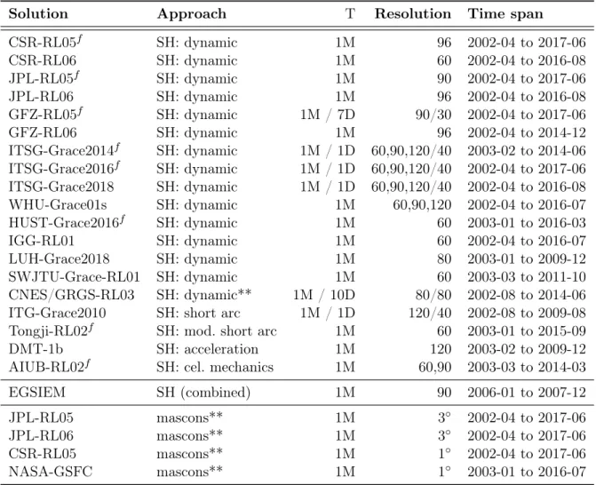
2.3 GRACE Analysis Centers and GRACE Solutions . . . . 10

3 Related Work 13 3.1 Validation of Hydrological Models Using GRACE Data . . . . 13

3.1.1 Total Water Storage Time Series . . . . 14

3.1.2 K-Band Range Rate Residuals . . . . 15

3.2 Assimilation of GRACE Data into Hydrological Models . . . . 16

4 Modeling Terrestrial Water Storage 23 4.1 Community Land Model version 3.5 . . . . 23

4.1.1 Model Structure . . . . 24

4.1.2 Water Balance . . . . 25

4.1.3 Model Setup . . . . 28

4.2 Global Hydrological Models . . . . 31

4.2.1 WGHM . . . . 31

4.2.2 LSDM . . . . 31

4.2.3 GLDAS Land Surface Models . . . . 31

4.3 Validation Data Sets . . . . 32

4.3.1 Soil Moisture . . . . 32

4.3.2 Discharge . . . . 33

4.3.3 Evapotranspiration . . . . 35

5 Processing of GRACE Data 37 5.1 Computing Gridded Total Water Storage Anomalies from GRACE Level-2 Data 37

5.1.1 From Gravity Potential to Total Water Storage Anomalies . . . . 38

5.1.2 Coefficients of Lower Degree . . . . 40

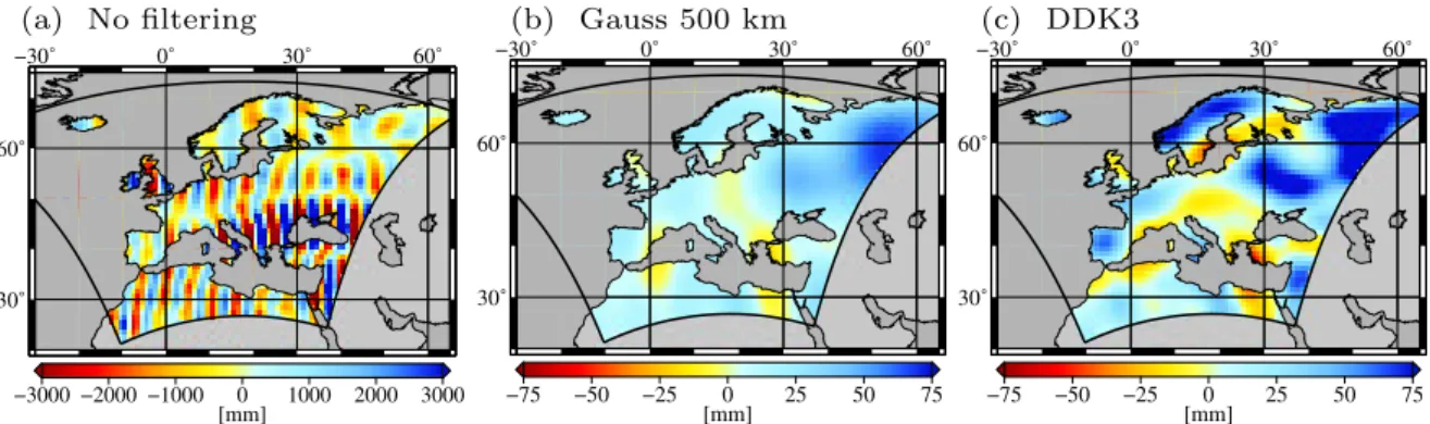
5.1.3 Removing Correlated Errors . . . . 41

5.1.4 Glacial Isostatic Adjustment . . . . 46

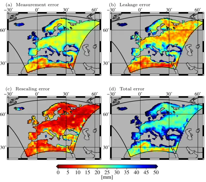
5.1.5 Error Propagation . . . . 47

5.2 Computing K-Band Residuals from GRACE Level 1B Data . . . . 53

5.2.1 Preparation of GRACE Level 1B Data . . . . 53

5.2.2 Computation of K-band Residuals . . . . 54

5.2.3 Evaluation of K-band Residuals . . . . 54

6 Concepts of Sequential Data Assimilation 57 6.1 Ensemble Kalman Filter Approaches . . . . 58

6.1.1 The Extended Kalman Filter . . . . 59

6.1.2 The Ensemble Kalman Filter . . . . 60

6.1.3 The Ensemble Transform Kalman Filter . . . . 61

6.1.4 The Singular Evolutive Interpolated Kalman Filter . . . . 62

6.1.5 The Error Subspace Transform Kalman Filter . . . . 62

6.1.6 Smoother Extensions . . . . 63

6.2 Tuning of the Filter Algorithms . . . . 63

6.2.1 Localization . . . . 63

6.2.2 Covariance Inflation . . . . 65

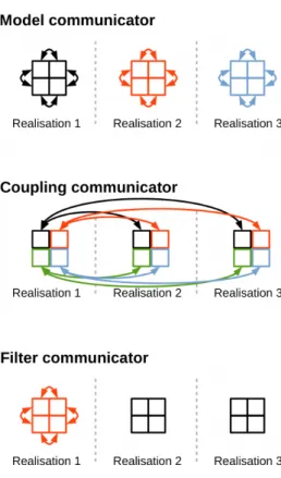
7 Implementing the Assimilation of GRACE Data into CLM3.5 67 7.1 The Assimilation Framework TerrSysMP-PDAF . . . . 69

7.2 Interface for Assimilating Total Water Storage Anomalies . . . . 72

7.2.1 State Vector . . . . 72

7.2.2 Observation Files . . . . 72

7.2.3 Observation Operator . . . . 73

7.2.4 Model Update . . . . 76

7.3 Generating an Ensemble of Model Runs with CLM3.5 . . . . 78

7.3.1 Initial Conditions . . . . 79

7.3.2 Atmospheric Forcings . . . . 79

7.3.3 Soil Texture . . . . 81

8.1 Validation Metrics . . . . 86

8.2 Assimilation of Synthetic Total Water Storage Observations . . . . 88

8.2.1 Twin Experiments . . . . 88

8.2.2 Influence of Data Assimilation on the TWS Compartments . . . . 91

8.2.3 Influence of the Ensemble Size . . . 101

8.2.4 Influence of Assimilation Algorithm and Observation Error Model . . . 104

8.2.5 Influence of Localization Radius and Inflation Factor . . . 109

8.2.6 Influence of the Observation Grid . . . 112

8.2.7 Influence of Data Assimilation on Sub-Monthly TWS Variability . . . 115

8.2.8 Influence of Biases in Precipitation Forcings . . . 116

8.2.9 Influence of Phase Shifts between Model and Observations . . . 117

8.2.10 Key Messages of Synthetic Assimilation Experiments . . . 118

8.3 Assimilation of GRACE-Derived Total Water Storage Observations . . . 120

8.3.1 Set-up of Assimilation Experiments with Real GRACE Data . . . 120

8.3.2 Comparison of GRACE Data and Output from the Assimilated Model 121 8.3.3 Analysis of Assimilation Increments . . . 124

8.3.4 Validation against Soil-Moisture Observations . . . 125

8.3.5 Validation against Discharge Gauges . . . 132

8.3.6 Validation against Evapotranspiration Observations . . . 134

8.3.7 Examples for Spatial and Temporal Downscaling of GRACE Observations137 8.3.8 Key Messages of GRACE Assimilation Experiments . . . 138

9 Validation of Offline and Assimilated Hydrological Models Using GRACE In-Orbit Residuals 141 9.1 In-Orbit Validation of Global Hydrological Models . . . 144

9.1.1 Time Series of Residuals . . . 144

9.1.2 Spatial Residual Analysis . . . 144

9.1.3 Regional Time Series of Residuals . . . 146

9.2 In-Orbit Validation of Short-Term Hydrological Variability . . . 149

9.3 In-Orbit Validation of Hydrological Signals from Reservoirs . . . 151

9.4 In-Orbit Validation of Data Assimilation Results . . . 153

9.5 Key Messages of the Analysis of KBRR and KBRA Residuals . . . 155

10 Conclusions and Outlook 157 10.1 Summary . . . 157

10.2 Conclusions . . . 158

10.3 Outlook . . . 160

Acronyms 165

List of Figures 175

List of Tables 177

Bibliography 200

Introduction

1.1 Motivation

Terrestrial water storage is a key variable of the global water cycle. The total water storage (TWS) on the continents includes all water components on and underneath the Earth’s sur- face, i.e. groundwater, soil moisture, surface waters (wetlands, rivers, lakes), snow water, and canopy water. Changes in TWS directly affect freshwater availability (Döll et al., 2016; Solan- der et al., 2017; Rodell et al., 2018), and can be related to natural disasters such as droughts and floods (Leblanc et al., 2009; Chew and Small, 2014; Sun et al., 2017). In addition, TWS changes are an important indicator for climate change (Green et al., 2011; Teutschbein et al., 2011; Yang et al., 2015; Kusche et al., 2016). Given the strong interconnection between human life and the terrestrial water cycle, millions of people are affected by natural disasters that can be expressed through TWS change. Well-documented examples are the California drought (Nelson and Burchfield, 2017), and the increasing intensity and duration of monsoon floods in South Eastern Asia (Dewan, 2015).

Changes in TWS and its components are associated with changes in hydrological fluxes, such as infiltration rates, runoff, groundwater recharge, and evapotranspiration. Indirectly, changes in TWS components also affect the atmospheric part of the water cycle and the Earth’s energy cycle. Soil moisture feedbacks on the atmosphere change variables such as air temperature and wind speed. Snow cover affects surface albedo and, thereby, induces changes in atmospheric circulation. Due to its memory effect, groundwater has a huge impact on long-term climate variability. Groundwater recharges soil moisture and, thus influences near-surface processes such as land-use change. Clearly, TWS is linked to a number of variables that were defined as Essential Climate Variables (ECV) by the Global Observing System for Climate (GCOS) under the auspices of United Nations organizations (Bojinski et al., 2014).

Accurate knowledge of TWS and TWS changes is indispensable for sustainable land and water management. Projections of TWS evolution are a basis for developing strategies that guarantee food and water supply, protect human health, preserve ecosystems, control energy generation and prevent migration streams. Finally, monitoring TWS directly targets the United Nation’s sustainable development goal 6, i.e. “ensure availability and sustainable management of water and sanitation for all”

.

Despite the importance of TWS, its monitoring is challenging. Hydrological models, which map the terrestrial water cycle, are only a simplified representation of reality and suffer from

1

https://unstats.un.org/sdgs/report/2018/goal-06/

the limited quality of input data. In-situ observations of TWS are sparse and represent point- wise measurements. TWS observations from remote sensing are available from the Gravity Recovery and Climate Experiment (GRACE) mission, but have a limited spatial and tempo- ral resolution and, thus, do not resolve fast hydrological processes at small spatial scales.

Based on these constraints, the motivation of this thesis is to enhance our knowledge about the evolution of TWS and the understanding of hydrological processes, combining both ob- servations and models.

1.2 Terrestrial Water Cycle and Space Gravimetry

Our knowledge of the terrestrial water cycle is based on two complementary elements: (i) observations from in-situ stations or remote sensing and (ii) physical laws represented by nu- merical models.

Hydrological models map the individual components of TWS and simulate water and energy fluxes. Conceptual hydrological models are based on empirical equations and parameters, and were developed for water resources management, as such, they often also model human water use. Hydrological land-surface models aim to represent physical processes of the real world by using mathematical equations. Hydrological models are run at different spatial scales (grid cells of a few meters to a hundred kilometers) and different temporal scales (hourly to monthly time steps). Uncertainties exist due to insufficient realism of model equations and structure, imperfect model parameters, and imperfect forcing and surface data sets. These uncertainties lead to deficiencies in representing trends and temporal variability of TWS. As a consequence, simulations from individual hydrological models differ largely (Schewe et al., 2013; Scanlon et al., 2018).

The GRACE mission (2002 – 2017) allowed the monitoring of large scale changes in the inte- gral sum of TWS (hydrosphere, biosphere, atmosphere, and oceans) from space. GRACE was a geodetic mission that observed the Earth’s time-variable gravity field by measuring changes in the distance between two satellites. These changes can be converted to TWS variability (Wahr et al., 1998). The temporal resolution of GRACE solutions is typically one month with a spatial resolution of a few hundred kilometers. Depending on the analysis strategy, daily GRACE solutions can be provided, but with a loss in spatial resolution. Decomposition of GRACE observations into individual components of TWS and to smaller spatial and tempo- ral scales requires complementary information from models, e.g. via statistical decomposition techniques (Rietbroek, 2014; Forootan et al., 2014).

The joint evaluation of hydrological models and GRACE-derived TWS variability has been beneficial for our knowledge about the terrestrial water cycle. Comparing modeled and ob- served TWS variability provides information on model deficiencies (Niu and Yang, 2006;

Alkama et al., 2010; Zhang et al., 2017). Calibrating hydrological model parameters against GRACE observations (usually model parameters have been calibrated against discharge ob- servation) helps to improve the representation of the terrestrial water cycle in the models (Werth et al., 2009; Chen et al., 2017).

Merging hydrological models and GRACE observations via data assimilation, i.e. modifying

the model state towards the observations in an optimal sense via a dynamical model, implies

(i) disaggregation of GRACE observations vertically, horizontally, and temporally, and (ii) a

more realistic representation of TWS compartments in the model with the potential to im-

prove also modeled water fluxes (Zaitchik et al., 2008; Girotto et al., 2016; Schumacher et al.,

2016). Therefore, GRACE-assimilating hydrological models provide unique information on the

distribution and redistribution of water.

1.3 Scientific Context and Objectives of the Thesis

Assimilating GRACE data into hydrological models presents several challenges. The tempo- ral and spatial (horizontal and vertical) resolution mismatch between simulated model states and observed TWS variability requires the use of sophisticated strategies to connect them (Girotto et al., 2016). Furthermore, data assimilation requires information on uncertainties of model and observations. The model error is difficult to quantify as it depends on uncer- tainties in model structure, atmospheric forcings, and soil data sets. GRACE-derived TWS maps are contaminated with correlated noise, which requires careful post-processing of the GRACE solutions. Currently, no standard way exists for the assimilation of GRACE data into hydrological models.

So far, only few groups have assimilated GRACE data into a hydrological model. Typically, the applied hydrological models have a spatial resolution between 0.5

( ∼ 50 km) to 1

( ∼ 100 km) and run at daily time steps, whereas the resolution of climate data might be restricted (e.g., number of cloud-free days per month, precipitation averaging). At our institute, GRACE data was assimilated into the conceptual WaterGAP Global Hydrology Model (WGHM) at 0.5

resolution (Schumacher, 2016). One exception for assimilation experiments at higher spatial resolution is the assimilation of GRACE data into a lumped rainfall-runoff model set up for the Rhine catchment at 1 km resolution, which however uses atmospheric forcing data resolved at 0.25

to 0.5

(Tangdamrongsub et al., 2015). Another example is the catchment-based land surface model running at a 1/8

degree grid with 15 minute time steps and daily atmospheric forcing data (Kumar et al., 2016).

This thesis aims at assimilating GRACE-derived TWS variability into the Community Land Model version 3.5 (CLM3.5) at 12.5 km spatial resolution over the entire of Europe using 3- hourly atmospheric forcing data. CLM3.5 is a physics-based land-surface model, which has a more complex structure than conceptual models like WGHM, as several hydrological, biogeo- physical, and biogeochemical processes are represented and water is stored in ten soil layers and up to five snow layers. Physical relationships between model variables cause particular challenges regarding a physically consistent update of the model states during assimilation.

CLM3.5 is part of the Terrestrial Systems Modeling Platform (TerrSysMP), which also in- cludes a groundwater component and an atmospheric model (Gasper et al., 2014; Shrestha et al., 2014). Including the assimilation of GRACE data into CLM3.5 using TerrSysMP will allow for extending the experiments to the groundwater component, or even to simulations of the whole terrestrial water cycle, i.e. simulations with a fully coupled model that includes atmospheric, land-surface, and groundwater components.

Previous studies investigated different strategies of assimilating GRACE data by varying gov- erning parameters such as, the assimilation algorithm (Khaki et al., 2017a), correlated versus white observation noise (Schumacher et al., 2016), and the observation grid (Khaki et al., 2017b). This thesis goes further and provides a systematic study of the most important as- similation parameters, which results in a ranking of their influences on the assimilation results.

This thesis addresses two main issues:

1. What is the optimal way of assimilating GRACE data into a high-resolution (12.5 km) continental scale land-surface model in terms of an improved description of water storage variability?

2. What is the impact of the assimilation of GRACE data on the performance of CLM3.5

in terms of the realism of simulated water storage compartments and water fluxes?

For answering the first question, a detailed review on the findings from previous GRACE assimilation studies is performed and, subsequently, a number of synthetic experiments are carried out. The second question is answered by validating water storage compartments and water fluxes of CLM3.5 against independent observation-based data sets, both before and after data assimilation.

Finally, this thesis provides an unprecedented reanalysis of TWS and its components at 12.5 km resolution and (sub-) daily time steps over Europe for the time span 2003 to 2010.

1.4 Organization of the Thesis

The thesis starts with an introduction into the characteristics of the GRACE mission (Chap- ter 2). The GRACE measurement principle is explained and different concepts of gravity field processing are introduced. The chapter concludes with an overview of recent GRACE solutions. Chapter 3 discusses studies related to the validation of hydrological models using GRACE observations and aims at a complete survey of studies that assimilate GRACE data into hydrological models. In Chapter 4, the structure and setup of CLM3.5 are explained and different global models are introduced, followed by an overview of the observation-based data sets that are used for model validation.

In Chapter 5 the processing of GRACE data, as performed in this thesis, is described in two parts: First, the computation of gridded TWS anomalies from GRACE spherical harmonics and corresponding error information is explained. Second, the processing of GRACE level 1B data for hydrological model validation is outlined. Chapter 6 gives an overview on individual data assimilation algorithms and tuning approaches. The strategy for assimilating GRACE data into CLM3.5, which was realized within this thesis, is explained in Chapter 7.

The results from data assimilation experiments are provided in Chapter 8. First, synthetic

experiments addressing the influence of different assimilation strategies are evaluated. Then,

modeled trends and phase shifts with respect to GRACE-derived TWSA are investigated

before and after data assimilation. Finally, the real-case scenario, an 8-year (2003 to 2010)

assimilation run, is validated against independent observations. Additionally, the representa-

tion of extreme events is assessed for the assimilated model. In Chapter 9 hydrological signals

are investigated for their skill in explaining level 1B GRACE K-band observations. First,

global hydrological models are assessed and then the CLM3.5 over Europe is evaluated with

respect to the impact of data assimilation. The thesis closes with a summary, followed by final

conclusions and an outlook on future possible extensions of this work (Chapter 10).

Gravity Recovery and Climate Experiment GRACE

2.1 GRACE Satellite Mission

The Gravity Recovery and Climate Experiment (GRACE) mission measured spatial and tem- poral variations of the Earth’s gravity field from March 2002 to June 2017. Variations in gravity are due to mass changes in hydrosphere, atmosphere, biosphere, oceans, and due to mass variations inside of the Earth. Monthly high-resolution gravity field solutions contribute to better knowledge about climate-relevant parameters and processes:

• Groundwater depletion and droughts threaten sustainable water supply and food pro- duction in many regions of the world, like e.g. California, Southern Europe, the Middle East, Africa, India, parts of China, and Australia (Mekonnen and Hoekstra, 2016).

GRACE is recognized as a unique tool for measuring changes of water resources on the continents with global coverage. The satellite mission measured the total sum of groundwater, soil moisture, snow, canopy water, and surface waters. An outstand- ing example for the potential of the GRACE mission was the combination of GRACE and ancillary observations with hydrological modeling in order to quantify groundwater depletion in the Northwest India Aquifer and to relate it to human activities (Rodell et al., 2009; Long et al., 2016). Furthermore, the joint evaluation of GRACE observa- tions and hydrological models enhanced the reliability of drought indicators and flood potential (Houborg et al., 2012; Reager et al., 2014). This highlights that both society and economy benefit from the measurements of the GRACE mission.

• The atmospheric-terrestrial flux , precipitation ( P ) minus evapotranspiration ( E ), is a key component for investigating the interaction between atmosphere and land surface, and for understanding human influences on climate change, e.g., via land use change.

However, in particular evapotranspiration is still not well known from observations and often poorly represented by Numerical Weather Prediction (NWP) model simulations.

By combining GRACE data with P − E and river discharge R the closure of the water

budget equation can be assessed (Lorenz et al., 2014; Springer et al., 2014, 2017; Lv

et al., 2017). Furthermore, trends in P , E , and R indicate that fluxes move away from an

equilibrium state. This might lead to an intensification of the water cycle. Accelerations

in total water storage can be derived from GRACE observations and allow the validation

of such trends in water fluxes (Eicker et al., 2016).

• River discharge is an important indicator for freshwater availability along rivers and of major importance for water management. As runoff from the continents occurs mainly at the river mouths, it acts as a driver for regional oceanic circulations (Carton, 1991), which are also of major importance for forcing climate models. Solving the water budget equation for R using GRACE data is one possibility for overcoming the problem of the decreasing number of gauging stations (Syed et al., 2009).

• Ocean currents transport heat and mass from the equator toward the poles, and, thus, regulate global and regional climatic conditions. GRACE emerged as valuable tool for quantifying changes in strength and direction of ocean currents and for validating ocean circulation models (Landerer et al., 2015).

• Sea level rise contaminates aquifers and agricultural soils and reshapes the world’s shorelines, which causes each year the displacement of thousands of people living in coastal areas. Ocean mass changes derived from GRACE observations allow us to moni- tor global and regional mass induced sea level variations (Lombard et al., 2007; Johnson and Chambers, 2013). One-half to two-thirds of sea level rise is attributed to mass loss from glacier and ice sheets (Gardner et al., 2013). GRACE observes glacier and ice sheet melting and, thus, also contributes to the decomposition of the sea level budget (Rietbroek et al., 2016).

GRACE was a joint mission of National Aeronautics and Space Administration (NASA) and Deutsches Zentrum für Luft- und Raumfahrt (DLR). The University of Texas Center for Space Research (CSR) was responsible for the overall GRACE mission. The project management was carried out by the Jet Propulsion Laboratory (JPL) and the German mission contributions were supplied by GeoForschungsZentrum (GFZ) in Potsdam. CSR, JPL, and GFZ are part of the GRACE Science Data System (GSDS), which is responsible for system development, data processing, and data archival (Bettadpur, 2012b).

GRACE consisted of two identical satellites, chasing each other with a distance of about 220 km on the same near circular orbit (Figure 2.1). The 89

orbit inclination ensured near- global coverage (Tapley et al., 2004a). The initial height of 500 km decreased down to 330 km by mid-2017 due to atmospheric drag. The low orbit permitted detailed mapping of anomalies of the gravity field down to spatial scales of a few hundred kilometers. The orbital period of about 94 minutes ensured dense spatial coverage after 30 days of continuous observations.

GRACE realized the low-low Satellite-to-Satellite Tracking (SST) concept. In an idealized case (i.e. no atmospheric drag, no solar radiation pressure, etc.), the change in distance between two co-orbiting satellites is nearly proportional to the difference in the Earth’s gravitational potential at the respective locations (Wolff, 1969). When the leading satellite approaches a positive gravity anomaly, it is attracted towards the anomaly and the distance to the trailing satellite increases. The distance decreases, when the trailing satellite is also attracted towards the gravity anomaly.

The key instrument of the GRACE satellites was a dual one-way K-band microwave ranging (KBR) system, which measured the inter-satellite range and its derivatives (Figure 2.2). The KBR system of each satellite was equipped by a horn antenna that transmitted carrier phase signals on two different frequencies. The phase measurements at each frequency are the ba- sis for deriving inter-satellite biased ranges with an accuracy of 1 µm. Subsequently, biased ranges from both frequencies are combined for removing ionospheric effects. After compres- sion, biased ranges, range-rates and range accelerations are available at 5 second sampling.

Non-gravitational forces acting on the satellites, such as air drag and solar radiation pressure,

are accounted for by measurements from accelerometers, which were located at the center

of mass of each satellite. Besides that, each satellite was equipped with two simultaneously

Figure 2.1: Measurement principle of the GRACE mission (Source: http://www2.csr.utexas.edu).

operating star cameras, which provided the internal orientation of the satellites with respect to their line of sight. Additionally, precise orbit determination and time tagging of all sensors was achieved with Global Positioning System (GPS) space receivers. In the end, the Earth’s gravity field can be computed from measured ranges and from the satellite’s accelerations, orientations, and positions (see Section 2.2).

Figure 2.2: Design of a GRACE satellite (Source: http://op.gfz-potsdam.de).

Initially, the GRACE mission was designed for a 5 year life period (Tapley et al., 2004b, 2016).

Since 2011, battery issues lead to missing solutions approximately every 6 months. Finally,

GRACE was operative until June 2017 providing 15 years of continuous records. An overlap

period with the GRACE Follow-On (GRACE-FO) mission, launched in May 2018, was not

achieved. Strategies for closing the gap include the computation of gravity field solutions from kinematic orbits of the Swarm Earth Explorer satellites (Lück et al., 2018). GRACE-FO now carries on the observation strategy of the GRACE mission, at the same time testing a new laser ranging system, which is more precise than the K-band instrument (Sheard et al., 2012;

Tapley et al., 2016). First GRACE-FO gravity solutions are expected to become available beginning of 2019.

2.2 GRACE Data Processing

Before the data collected on board of the GRACE satellites can be used for gravity field in- vestigations, several correction and filtering steps are required (Bettadpur, 2012b). Depending on the processing state, the data products are divided into five different categories:

• Level 0: The level 0 data products are raw data, which were received by the GRACE Raw Data Center (RDC) at DLR in Neustrelitz (Germany) via telemetry at each pass of the satellites. The down-link from each satellite includes one file with science instrument data and one file with spacecraft housekeeping data.

• Level 1A: The binary encoded measurements from the level 0 data products are con- verted to engineering units and time tagged to Global Positioning System (GPS) time.

Furthermore, quality control flags are added and the data are reformatted for further processing.

• Level 1B: Level 0 and level 1A data products are transformed into a uniform reference system and the sampling of the data products is reduced by temporal filtering. Be- sides, ancillary data sets like preliminary orbit information belong to the level 1B data products.

• Level 2: Level 2 data products provide gravity field solutions derived from level 1B data on the basis of spherical harmonic coefficients or other base functions.

• Level 3: Gridded time series of total water storage (TWS) variations are obtained from level 2 data products by applying post-processing steps, like e.g. spatial filtering. These products typically have a spatial resolution of a few hundred kilometers and a temporal resolution of one month.

The different categories of GRACE products address the needs of different user groups, which vary from the improvement of gravity field estimation techniques based on level 1B data to mere applications of level 3 data for e.g. hydrological studies. In this thesis, level 1B data (see Section 5.2) and of level 2 data (see Section 5.1) are used.

Different strategies exist for the computation of gravity field solutions from KBR, GPS, star camera, and accelerometer observations. All approaches are based on Newton’s equation of motion, which relates the orbit of a satellite of mass m to the forces acting on the satellite for any given time t ,

¨ r = 1

m f (t, r, ˙r), (2.1)

with r , ˙r , and ¨ r denoting the satellite’s position, velocity and acceleration, respectively. The

force function f includes gravitational (conservative) accelerations and non-gravitational (non-

conservative) accelerations. In general, a two-step approach is applied to derive gravity field

solutions (Bettadpur, 2012a):

1. The orbit of each satellite is derived by numerical integration of the equation of motion, considering an apriori mean static gravity field model in combination with so-called background force models that represent forces from tides and from non-tidal oceanic and atmospheric mass variations. Generally, the following background models are taken into account (see e.g.; Dahle et al., 2012; Bettadpur, 2012c; Watkins and Yuan, 2014):

• N-Body Perturbations : The satellites’ orbits are influenced by gravitational forces from third bodies, i.e. the sun, the moon, and the planets. Tidal forces also act on the Earth and cause mass variations, which, in turn, influence the satellite.

Direct and indirect accelerations acting on the GRACE satellites are computed from planetary ephemerides (Agnew, 2010).

• Solid Earth Tides : Tidal forces induce deformations of the solid Earth, which can be modeled using Love numbers (Wahr, 1981). Subsequently, the influence on the gravitational potential is computed.

• Ocean Tides : Oceanic mass variations due to tidal forces are taken into account by combining models of the different tidal constituents.

• Pole Tides : Changes in the Earth’s rotation result in changes of the centrifugal force. The influence on the gravitational potential is computed from the polar motion and (i) an Earth model for the contribution of the solid Earth and (ii) an equilibrium model for the oceanic contribution (Desai, 2002).

• De-aliasing : High-frequency (< 30 days) non-tidal variations of atmosphere and ocean are modeled and removed using the Atmosphere and Ocean De-aliasing Level- 1B (AOD1B) product (Flechtner et al., 2015; Dobslaw et al., 2017a). By this means, aliasing of high frequencies into monthly gravity field solutions is avoided.

• Non-gravitational Forces : Non-gravitational accelerations, i.e. atmospheric drag and radiation pressure from Sun and Earth, were measured by the accelerometers on-board of the satellites. A few-parameter model relating linear acceleration ob- servations to non-gravitational forces is set up. During gravity field estimation, biases and scale factors of the accelerometer measurements are co-estimated.

• Relativistic Correction : Instead of a fully consistent relativistic formulation of the equation of motion, general relativistic corrections are applied as described in Chapter 10 of the IERS 2010 conventions (Petit and Luzum, 2010).

2. Residuals are computed between the predicted orbit and the GPS and KBR observations.

Observation equations that relate gravity field parameters and additional parameters to the residuals are linearized and solved within an iterative least squares adjustment.

Popular approaches for setting up the observation equations are (i) the classical variational or

dynamic approach (Riley et al., 1967; Bettadpur and McCullough, 2017), (ii) the acceleration

approach (Ditmar and van der Sluijs, 2004; Weigelt, 2017), and (iii) the energy balance ap-

proach (Jekeli, 1999, 2017). For the classical variational approach, a so-called state transition

matrix is set up that relates the residuals to variations in the gravity field parameters and to

initial conditions for the satellites’ positions and velocities. Then, corrections to the gravity

field parameters are computed iteratively by integrating the variational equations. Hereby,

initial conditions are estimated for individual arcs, which have typically a length between 6

and 24 hours as a trade-off between linearization errors and the number of unknowns. Instead

of solving the variational equations, the acceleration approach directly links range accelera-

tions to gravity gradients. In doing so, linearization errors are avoided and the computational

costs are limited as no iterations are necessary. However, the double differentiation amplifies

the noise, making more sophisticated data processing necessary. The energy balance approach

is based on the conservation of potential and kinetic energy of a satellite constellation. The main idea is to represent the Earth’s gravitational potential as work acting on the satellites.

Again, integration of the variational equations and iterations are redundant, but the noise situation is challenging in the inversion process.

Variants of the variational approach are the short arc approach (Mayer-Gürr, 2006) and the modified short arc approach (Chen et al., 2015), which minimize model errors using very short arcs between 30 minutes and 2 hours. The acceleration apporach was extended by Liu (2008) to the average acceleration approach that includes smoothing of the satellites’ orbits and con- siders a noise model for data weighting. Finally, the celestial mechanics approach (Beutler et al., 2010a,b) solves for the gravity field parameters in a generalized orbit determination problem and is based on the Bernese GPS Software (Dach et al., 2007).

All of the above approaches yield at estimating spherical harmonic coefficients for representing the gravity field. A particular challenge of the GRACE mission is the measurement configu- ration, which leads to stripes and requires careful post-processing and spatial filtering of level 2 data (see Chapter 5). An alternative approach to the estimation of spherical harmonic coef- ficients are so-called mass concentration blocks (mascons), which are regularized solutions of the gravity field. Measured range-rates or range-accelerations are directly fit to specified grid locations while applying geophysical or data-driven constraints (Watkins et al., 2015; Wiese et al., 2016; Luthcke et al., 2014; Save et al., 2016).

After more than 15 years of GRACE data evaluation, the processing strategies and back- ground models still evolve. In particular the AOD1B product for high-frequency non-tidal mass transport in the atmosphere and oceans is developed further (Dobslaw et al., 2017a) with first studies taking also hydrological variability into account (Zenner et al., 2014). More- over, strategies for handling non-conservative forces become more and more elaborate (Chen et al., 2016; Klinger and Mayer-Gürr, 2016). Another example for the improvement of the processing strategy is the refinement of orbit integration, which is necessary for linearization of the observation equations (Ellmer and Mayer-Gürr, 2017).

2.3 GRACE Analysis Centers and GRACE Solutions

The three official processing centers within the GSDS are GFZ, JPL, and CSR. They published the reprocessed GRACE RL06 in 2018. Improvements with respect to RL05 were achieved in particular through the improved de-aliasing product AOD1B-RL06 (Dobslaw et al., 2017b).

All of the official processing centers use the classical variational approach (or dynamic ap- proach) for deriving monthly sets of spherical harmonic coefficients. However, the individual solutions differ regarding the processing strategy, the background models and the spectral res- olution. Besides, several other groups compute their own gravity field models with alternative approaches and with different spatial and temporal resolution.

Table 2.1 gives an overview on selected gravity field solutions. The temporal resolution of the

gravity field solutions vary between one month (1M) and one day (1D) (column 3). The spa-

tial resolution is between degree and order (d/o) 30 to 120 for solutions provided as spherical

harmonic (SH) coefficients (column 4). The corresponding wavelengths λ can be computed

with the Earth’s radius R and and the maximum degree n

according to λ = (πR/n

) .

Solutions up to n

=30 cover wavelengths down to 670 km and solutions up to n

=120

cover wavelengths down to 170 km, respectively. Some of the solutions provided as spherical

harmonic coefficients are available after filtering in spectral domain, which is indicated by

the index

in column 1. The mascon solutions are provided on 1

and 3

grids. Please note

that the actual spatial resolution of GRACE data is difficult to quantify due to the spatial

correlation structure and furthermore depends on the latitude. In general, at the equator a resolution of about 300 km is assumed.

The dynamic approach is used by the three official processing centers and by the Graz Univer- sity of Technology (ITSG-Grace2014, ITSG-Grace2016, ITSG-Grace2018; Mayer-Gürr et al., 2016, 2018), the GNSS Research Center of Wuhan University (WHU-Grace01s; Zhou et al., 2015), the Huazhong University of Science and Technology (HUST-Grace2016; Zhou et al., 2016), the Institute of Geodesy and Geophysics at the Chinese Academy of Sciences (IGG- RL01; Wang et al., 2015), the Leibniz University Hannover (LUH-GRACE2018; Naeimi et al., 2018), the Faculty of Geoscience and Environment Engineering at Southwest Jiaotong Univer- sity (SWJTU-Grace-RL01), and the Space Geodesy Research Group (CNES/GRGS; Lemoine et al., 2007; Bruinsma et al., 2010). ITSG and WHU-Grace2016 provide monthly solutions for d/o 60, 90, and 120. ITSG solutions also include daily solutions, which are estimated within an Kalman smoother framework using temporal correlation patterns derived from geophyical models (Kurtenbach et al., 2012). Additionally, ITSG-Grace2016 is provided with full covari- ance information. Besides the three official processing centers, ITSG-Grace2018 is currently the only publicly available solution that uses the AOD1B-RL06 product instead of AOD1B- RL05. Unlike other solutions, the CNES/GRGS-RL03 gravity fields are constrained towards a mean field, which stabilizes the solutions and makes filtering unnecessary (indicated by the

** in Table 2.1).

Bonn University (ITG-Grace2010) and Tongji University (Tongji-RL02; Chen et al., 2015, 2016) use the short-arc and modified short-arc approaches. Furthermore, ITG-Grace2010 pro- vides daily solutions, which are based on the same method as ITSG-Grace2016 (Kurtenbach, 2011). Gravity field solutions based on the acceleration approach are published by Delft Uni- versity of Technology (DMT-1b; Liu, 2008; Liu et al., 2010) and solutions based on the celestial mechanics approach are computed at Bern University (AIUB-RL02; Meyer et al., 2016).

Sakumura et al. (2014) found that the combination of several gravity field solutions using the ensemble mean reduces the noise. The European Gravity Service for Improved Emergency Management (EGSIEM) combined for the first time gravity fields of different analysis centers (AIUB-RL02, GFZ-RL05, CNES/GRGS-RL03, ITSG-Grace2016) on normal equation level, while optimally weighting the individual solutions.

While mascon solutions of JPL (Watkins et al., 2015; Wiese et al., 2016) are constrained with information from geophysical models, CSR (Save et al., 2012, 2016) and NASA’s Goddard Space Flight Center (NASA-GSFC) (Luthcke et al., 2013, 2014) apply constraints that are exclusively based on GRACE data. CSR also computed a daily mascon product based on a sliding window approach, which is not yet publicly available (Sakumura et al., 2016).

Obviously, the question arises, which of the GRACE solutions should be used. This depends mainly on the application requirements. Several studies compare and validate GRACE solu- tions (e.g. Sakumura et al., 2014; Scanlon et al., 2016). Generally, a combined solution as de- rived by the EGSIEM project reduces noise and is more reliable. All products based on spher- ical harmonics require careful post-processing including filtering and signal restoration due to leakage effects. In contrast, filtering is not necessary when using Mascon solutions. However, these solutions are drawn towards constraints during the estimation process, which is an addi- tional error source. Most of the current global gravity field solutions can be downloaded from the ICGEM website ( http://icgem.gfz-potsdam.de/home ). ICGEM also provides an online tool to convert monthly spherical harmonic coefficients from individual solutions to gridded maps of gravity anomaly, TWS, etc. Furthermore, interactive tools for displaying and com- paring different GRACE solutions are available (e.g. http://www.thegraceplotter.com/ ).

Besides global gravity models, a number of regional solutions exist.

The different gravity field solutions allow some kind of quality control, but as all of them are based on the same level 1B data, they contain the same instrument errors and the same errors from atmospheric and oceanic de-aliasing products. Therefore, differences between the solu- tions cannot be used as error estimate. The error estimate of the GRACE solutions is indeed challenging and represents a specific field of research, which will be discussed in Section 5.1.5.

In this work, I use the solutions from ITSG-Grace2016 as they (i) cover the whole study period, (ii) are unconstrained solutions, (iii) provide full error covariance matrices, and (iv) also include a daily product. The full error covariance matrices are interesting for studying the influence of correlations in the context of data assimilation.

Table 2.1: This table provides an overview on the currently publicly available GRACE solutions (as of December 2018). The responsible institutions and references are given in the text. The index

in Column 1 indicates solutions of spherical harmonic (SH) coefficients that are also available after spectral filtering. Column 2 gives the approaches that are used for estimating the gravity field solutions (see Section 2.2). Constrained solutions are indicated by **. The temporal resolution of the products is provided in Column 3, where 1M indicates one month and 1D one day. For products provided as SH coefficients, the spatial resolution is indicated by the maximum degree of the SH coefficients, whereas for mascon products the grid size is given (Column 4).

Solution Approach T Resolution Time span

CSR-RL05

SH: dynamic 1M 96 2002-04 to 2017-06

CSR-RL06 SH: dynamic 1M 60 2002-04 to 2016-08

JPL-RL05

SH: dynamic 1M 90 2002-04 to 2017-06

JPL-RL06 SH: dynamic 1M 96 2002-04 to 2016-08

GFZ-RL05

SH: dynamic 1M / 7D 90/30 2002-04 to 2017-06

GFZ-RL06 SH: dynamic 1M 96 2002-04 to 2014-12

ITSG-Grace2014

SH: dynamic 1M / 1D 60,90,120/40 2003-02 to 2014-06 ITSG-Grace2016

SH: dynamic 1M / 1D 60,90,120/40 2002-04 to 2017-06 ITSG-Grace2018 SH: dynamic 1M / 1D 60,90,120/40 2002-04 to 2016-08

WHU-Grace01s SH: dynamic 1M 60,90,120 2002-04 to 2016-07

HUST-Grace2016

SH: dynamic 1M 60 2003-01 to 2016-03

IGG-RL01 SH: dynamic 1M 60 2002-04 to 2016-07

LUH-Grace2018 SH: dynamic 1M 80 2003-01 to 2009-12

SWJTU-Grace-RL01 SH: dynamic 1M 60 2003-03 to 2011-10

CNES/GRGS-RL03 SH: dynamic** 1M / 10D 80/80 2002-08 to 2014-06 ITG-Grace2010 SH: short arc 1M / 1D 120/40 2002-08 to 2009-08

Tongji-RL02

SH: mod. short arc 1M 60 2003-01 to 2015-09

DMT-1b SH: acceleration 1M 120 2003-02 to 2009-12

AIUB-RL02

SH: cel. mechanics 1M 60,90 2003-03 to 2014-03

EGSIEM SH (combined) 1M 90 2006-01 to 2007-12

JPL-RL05 mascons** 1M 3

2002-04 to 2017-06

JPL-RL06 mascons** 1M 3

2002-04 to 2017-06

CSR-RL05 mascons** 1M 1

2002-04 to 2017-06

NASA-GSFC mascons** 1M 1

2003-01 to 2016-07

Related Work

Over the past decade, the Gravity Recovery and Climate Experiment (GRACE) mission has contributed significantly to the understanding of hydrological processes (Tapley et al., 2004a).

In particular, a large number of studies has been using GRACE data as a validation tool for hydrological models (see Section 3.1). These studies are usually based on gridded or basin- averaged total water storage anomalies (TWSA, Section 3.1.1), and suffer from the downward continuation and filtering steps. To overcome these limitations, Eicker et al. (2016) evalu- ated global hydrological models in-orbit on the basis of level 1B data by computing K-band range-rate (KBRR) residuals. This approach was extended in this thesis to examining dif- ferent model versions and signals on smaller spatial scales. Section 3.1.2 introduces studies which assess different geophysical signals using KBRR residuals. With Zaitchik et al. (2008), a new application of GRACE data emerged, the assimilation of total water storage anomalies (TWSA) into a hydrological model, as also realized within this thesis. During the last few years, important progress has been made regarding the assimilation of GRACE data, but still only few studies have been published (Section 3.2).

3.1 Validation of Hydrological Models Using GRACE Data

Hydrological models aim at representing water, energy, and biogeochemical fluxes at differ- ent spatial and temporal scales, and thereby contribute to a better understanding of the Earth’s system. Total water storage (TWS) is one key variable of hydrological models as the distribution of water within the model controls all major hydrological processes. However, uncertainties in (i) model structure or representation of physical processes, (ii) model param- eters, and (iii) atmospheric forcing data lead to limited predicting skills. Before the start of the GRACE mission, validation of TWS simulated by hydrological models was restricted to few ground-based measurements.

Indeed, the start of the GRACE mission in 2002 has opened up new possibilities for assessing

the quality of hydrological models and for determining model deficiencies. Nevertheless, it

should be remembered that GRACE observed the spatio-temporal variability of the total sum

of the water column, whereas hydrological models simulate a number of individual storage

compartments. Furthermore, in contrast to hydrological models, which usually run at daily

to hourly time steps on grids of 1

or smaller, GRACE-derived TWSA are monthly data sets

with a spatial resolution of about 200 km. The resulting challenges are described in detail in

Section 5.1. Below, the records of hydrological model validation with GRACE data on the

basis of TWS time series are presented (Section 3.1.1), followed by an introduction into stud-

ies relevant for the validation of hydrological signals based on GRACE level 1B data (Section

3.1.2).

3.1.1 Total Water Storage Time Series

The very first studies comparing hydrological models and GRACE primarily explored the fundamental information content of the new type of observations provided by GRACE. In this scope, Andersen (2005) evaluated 15 months of gravity data and compared them to four hydrological models on an inter-annual scale. At that time, observations and models diverged widely, with only one out of four models being correlated with GRACE data at the global scale. In general, studies of this period were limited to comparing spatial maps of the sea- sonal cycle and basin-averaged TWSA time series of large river catchments, thereby verifying continental scale patterns and general seasonal dynamics (Tapley et al., 2004a; Wahr et al., 2004; Ramillien et al., 2004, 2005). Research tended to focus on basic GRACE processing strategies, e.g. filtering and treatment of the low-degree coefficients (Chen et al., 2005; Chen, 2005), rather than on hydrological phenomena.

A step forward was the assessment of specific hydrological extreme events in GRACE-derived TWSA and hydrological models. In an early study by Andersen et al. (2005) the manifestation of the 2003 European heat wave in GRACE data was confirmed by three independent data sets, which outlined the potential of GRACE for investigating extreme climate events. Chen et al. (2009) reported the 2005 Amazon drought being distinct in the GRACE time series, whereas, in this case, hydrological models failed in representing the drought related decline in TWS. Similarly, Chen et al. (2010) found a detailed picture of the 2008/2009 La Plata drought in the GRACE data, while this event was only partly captured by the investigated land surface model. A more recent study by Jin and Feng (2013) surveyed the general difficul- ties of global hydrological models in matching GRACE-derived trends and accelerations for regions affected by extreme events.

Several studies investigated the general performance of different model versions and/or dif- ferent hydrological models. In this scope, Niu and Yang (2006) used GRACE data to demon- strated the better performance of a modified version of the Community Land Model (CLM) compared to the standard version. The value of GRACE for detecting missing processes in hydrological models or improving existing ones was confirmed by Alkama et al. (2010), who carried out a statistical comparison between GRACE and a hydrological model for the 183 largest river basins of the world. Grippa et al. (2011) evaluated six GRACE solutions and soil moisture from nine land surface models over West Africa, and identified processes to be improved in the land surface modeling. Pokhrel et al. (2013) included an interactive ground- water store in a hydrological model over the Amazon basin and validated both model versions against GRACE, achieving significant improvement especially with respect to annual ampli- tudes and phases. Recently, Getirana et al. (2017) used GRACE data to prove the influence of rivers and floodplanes on TWS. General strengths and weaknesses of current global hydrologi- cal models were evaluated in a comprehensive study by Zhang et al. (2017), who compared the performance of four different models in 31 catchments situated within different climate zones.

Scanlon et al. (2018) showed that global hydrological models underestimate TWS trends rel- ative to GRACE observations.

Overall, a considerable number of studies suggested that hydrological models generally tend to underestimate the amplitude of TWS compared to GRACE and that they often have a time shift of about one month.

In recent years, decreasing errors in the GRACE solutions enabled the validation of hydro- logical models also at smaller spatial scales. This concurrently stimulated research regarding processing strategies for ensuring the consistency of GRACE data and output from hydrolog- ical models (Longuevergne et al., 2010).

Progress in the quality of the GRACE solutions also enabled the evaluation of individual

hydrological compartments. For instance, Jin and Feng (2013) computed ground water vari- ability from the difference of GRACE-derived TWSA and surface water, soil moisture, snow, ice and canopy water from two different hydrological models. They found one of the models representing a relatively reliable data set of groundwater variability compared to in-situ ob- servations. Similarly, Joodaki et al. (2014) estimated the human contribution to groundwater depletion in the Middle East. Döll et al. (2014b) contributed to a better understanding of groundwater depletion and its causes by jointly interpreting TWSA from GRACE and an im- proved global hydrological model, which considers groundwater recharge from surface water bodies and major aquifers.

Another step forward was the separation of GRACE-derived TWSA into different components using statistical decomposition techniques. Temporal and spatial decomposition of TWSA time series enables a more detailed evaluation of hydrological processes including interannual and non-periodic phenomena. For the first time, Rangelova et al. (2007) applied Principle Component Analysis (PCA) to GRACE data and to three hydrological models over North America. They found a strong annual signal in the first spatial mode due to snow accumula- tion and inter-annual mass changes in the second mode. For the hydrological models similar patterns were revealed, although they rather underestimated mass changes.

In later studies, the application of statistical decomposition techniques were extended from pure validation of hydrological models to joint evaluation of TWS observations and models in order to gain maximum information on hydrological dynamics in different storage compart- ments. Awange et al. (2014) applied PCA to TWSA from GRACE, to soil moisture from a hydrological model, and to remotely sensed precipitation. Hence, they concluded about the relationship between rainfall and ground water variations in Ethiopia. Forootan et al. (2014) went even further and separated water storage compartments over Iran by (i) decomposing data sets from hydrological modeling and altimetry into statistically independent components, and (ii) fitting them to TWSA from GRACE. Andrew et al. (2017) used a wavelet approach in order to partition TWSA from GRACE into its compartments. Recently, Felfelani et al.

(2017) isolated anthropogenic water storage changes from multiple GRACE solutions and two hydrological models, in which human factors were excluded. In particular, their results demonstrated different performance of the two models in highly-managed catchments and in snow-dominated regions.

Lately, there has been growing interest in the quantification of uncertainty of TWS products from GRACE and from hydrological models, respectively (Long et al., 2017). A further focus is put on deriving one ’best’ GRACE product and to make it available to a wider user com- munity, as attempted by the European Gravity Service for Improved Emergency Management (EGSIEM) project.

In this review, I highlighted a subjective selection of studies that represent the progress made in validating hydrological models since the start of the GRACE mission. An overview on all GRACE related publications including applications related to ocean and atmosphere is provided by GeoForschungsZentrum (GFZ) at http://www-app2.gfz-potsdam.de/pb1/op/

grace/references/sort_date.html.

3.1.2 K-Band Range Rate Residuals

Most of the above discussed studies assess monthly gravity field solutions provided either as

sets of spherical harmonic coefficients or as gridded values of equivalent water heights. Gravity

field processing requires downward continuation from the satellites’ altitude, which amplifies

high-frequency measurement errors. Consequently, the recovered gravity fields are noisy and

require a tailored filtering procedure. Filtering results into attenuated fields of monthly mass

variations at a coarse spatial resolution of a few hundred kilometers, which complicates com- parison with high-resolution geophysical or hydrological models. The limitations due to down- ward continuation and filtering can be overcome by comparing model outputs and GRACE observations directly on the basis of GRACE level 1B K-band observations. In this scope, K- band range-rate (KBRR) or K-band range-acceleration (KBRA) observations are simulated from modeled mass variations and subtracted from original GRACE K-band observations leading to KBRR or KBRA residuals.

Since the early years of the GRACE mission, KBRR residuals were evaluated to assess the quality of GRACE solutions, ocean models, atmospheric models, and of the GRACE de- aliasing products (Bosch et al., 2009; Zenner et al., 2012; Dobslaw et al., 2013). Therefore, the ability of different products in reducing KBRR residuals was compared. For instance, Kusche et al. (2009a) computed KBRR residuals for GRACE solutions filtered with different de-correlation filters. Filtering reduced the KBRR residuals, which was however inconclusive (Kusche et al., 2009a). More recently, Dobslaw et al. (2017b) used KBRA residuals to localize regions that are problematic for de-aliasing. However, KBRA are more noisy than KBRR due to differentiation, which is challenging regarding the evaluation of small signals.

Han et al. (2008) explained the computation of KBRR in detail and investigated hydrological signatures and signatures from glacial isostatic adjustment over South America, Africa, and North America. Moreover, Han et al. (2010a) detected signatures of the 2010 Maule (Chile) earthquake in the KBRR residuals. They investigated range-rate data close to the epicenter before and after the earthquake and were able to infer a negative gravity anomaly after the earthquake.

Different hydrological models were first evaluated using GRACE level 1B data in the stud- ies of Han et al. (2009) and Han et al. (2010b). They assessed individual arcs of range-rate residuals for the Amazon basin regarding the impact from surface waters and soil moisture.

Later on, Zenner et al. (2014) computed KBRR residuals for hydrological signals from two global hydrological models used in addition to the atmosphere and ocean de-aliasing product and compared them to KBRR residuals derived from the daily Kalman-based GRACE solu- tions of ITG-Grace2010 (Kurtenbach, 2011) used in addition to the atmosphere and ocean de-aliasing product. GRACE-derived ITG daily Kalman solutions turned out to better fit to GRACE KBRR observations than daily hydrological model output. At the moment it is not clear, whether daily hydrological model output could improve GRACE solutions through de-aliasing.

3.2 Assimilation of GRACE Data into Hydrological Models

Traditionally, hydrological models have been calibrated against discharge observations (Duan et al., 2006). Discharge reflects the response to all hydrological processes within a catchment.

However, models calibrated only with respect to discharge often fail in providing reliable es- timates of other relevant hydrological variables (Guo et al., 2017). Therefore, multi-objective calibration with complementary observations became more and more relevant. A decade ago, studies have started to investigate the integration of GRACE observations into the calibration process of hydrological models (e.g., Werth et al., 2009; Lo et al., 2010; Livneh and Letten- maier, 2012; Rakovec et al., 2016; Chen et al., 2017; and Bai et al., 2017), which generally results in an improved representation of the continental water cycle.

A step further in tuning models towards observations is taken by data assimilation, i.e. the

hydrological model states are updated towards the observations. Assimilation of GRACE

observations allows for improving model estimates of TWS while simultaneously disaggregat-