www.biogeosciences.net/13/3203/2016/
doi:10.5194/bg-13-3203-2016
© Author(s) 2016. CC Attribution 3.0 License.
Bathypelagic particle flux signatures from a suboxic eddy in the oligotrophic tropical North Atlantic: production,
sedimentation and preservation
Gerhard Fischer1,2, Johannes Karstensen3, Oscar Romero2, Karl-Heinz Baumann1,2, Barbara Donner2,
Jens Hefter2,4, Gesine Mollenhauer2,4, Morten Iversen2,4, Björn Fiedler3, Ivanice Monteiro5, and Arne Körtzinger3
1Geosciences Department, University of Bremen, Klagenfurter Str., 28359 Bremen, Germany
2Marum Centre for Marine Environmental Sciences, Leobener Str., University of Bremen, 28359 Bremen, Germany
3GEOMAR Helmholtz Center for Ocean Research Kiel, Düsternbrooker Weg 20, 24105 Kiel, Germany
4Alfred Wegener Institute, Helmholtz Center for Polar and Marine Sciences, 27570 Bremerhaven, Germany
5Instituto Nacional de Desenvolvimento das Pescas (INDP), Cova da Inglesa, CP132, Mindelo, São Vicente, Cabo Verde Correspondence to:Gerhard Fischer (gerhard.fischer@uni-bremen.de)
Received: 30 October 2015 – Published in Biogeosciences Discuss.: 13 November 2015 Revised: 28 April 2016 – Accepted: 13 May 2016 – Published: 2 June 2016
Abstract.Particle fluxes at the Cape Verde Ocean Observa- tory (CVOO) in the eastern tropical North Atlantic for the period December 2009 until May 2011 are discussed based on bathypelagic sediment trap time-series data collected at 1290 and 3439 m water depth. The typically oligotrophic par- ticle flux pattern with weak seasonality is modified by the appearance of a highly productive and low oxygen (mini- mum concentration below 2 µmol kg−1 at 40 m depth) anti- cyclonic modewater eddy (ACME) in winter 2010. The eddy passage was accompanied by unusually high mass fluxes of up to 151 mg m−2d−1, lasting from December 2009 to May 2010. Distinct biogenic silica (BSi) and organic carbon flux peaks of ∼15 and 13.3 mg m−2d−1, respectively, were ob- served in February–March 2010 when the eddy approached the CVOO. The flux of the lithogenic component, mostly mineral dust, was well correlated with that of organic car- bon, in particular in the deep trap samples, suggesting a tight coupling. The lithogenic ballasting obviously resulted in high particle settling rates and, thus, a fast transfer of epi-/meso- pelagic signatures to the bathypelagic traps. We suspect that the two- to three-fold increase in particle fluxes with depth as well as the tight coupling of mineral dust and organic car- bon in the deep trap samples might be explained by parti- cle focusing processes within the deeper part of the eddy.
Molar C : N ratios of organic matter during the ACME pas- sage were around 18 and 25 for the upper and lower trap
samples, respectively. This suggests that some productivity under nutrient (nitrate) limitation occurred in the euphotic zone of the eddy in the beginning of 2010 or that a local nitrogen recycling took place. Theδ15N record showed a de- crease from 5.21 to 3.11 ‰ from January to March 2010, while the organic carbon and nitrogen fluxes increased. The causes of enhanced sedimentation from the eddy in Febru- ary/March 2010 remain elusive, but nutrient depletion and/or an increased availability of dust as a ballast mineral for organic-rich aggregates might have contributed. Rapid rem- ineralisation of sinking organic-rich particles could have con- tributed to oxygen depletion at shallow depth. Although the eddy formed in the West African coastal area in summer 2009, no indications of coastal flux signatures (e.g. from di- atoms) were found in the sediment trap samples, confirming the assumption that the suboxia developed within the eddy en route. However, we could not detect biomarkers indica- tive of the presence of anammox (anaerobic ammonia ox- idation) bacteria or green sulfur bacteria thriving in photic zone suboxia/hypoxia, i.e. ladderane fatty acids and isore- nieratene derivatives, respectively. This could indicate that suboxic conditions in the eddy had recently developed and/or the respective bacterial stocks had not yet reached detec- tion thresholds. Another explanation is that the fast-sinking organic-rich particles produced in the surface layer did not interact with bacteria from the suboxic zone below. Carbon-
ate fluxes dropped from∼52 to 21.4 mg m−2d−1from Jan- uary to February 2010, respectively, mainly due to reduced contribution of shallow-dwelling planktonic foraminifera and pteropods. The deep-dwelling foraminiferaGloborotalia menardii, however, showed a major flux peak in February 2010, most probably due to the suboxia/hypoxia. The low oxygen conditions forced at least some zooplankton to re- duce diel vertical migration. Reduced “flux feeding” by zoo- plankton in the epipelagic could have contributed to the en- hanced fluxes of organic materials to the bathypelagic traps during the eddy passage. Further studies are required on eddy-induced particle production and preservation processes and particle focusing.
1 Introduction
Time-series particle flux studies have been performed in many ocean areas, including typical oligotrophic settings in the Atlantic and the Pacific (Karl et al., 1996; Neuer et al., 2007; Lampitt and Antia, 1997; Honjo et al., 2008) and in eastern boundary upwelling ecosystems (EBUEs, Freon et al., 2009) (Fischer et al., 2010; Romero et al., 2002). In gen- eral, seasonality is low in areas with low primary produc- tion, while it increases towards coastal and open ocean high production (equatorial, polar) settings (Berger and Wefer, 1990; Romero and Armand, 2010). Mass fluxes at the French oligotrophic EUMELI site located north-west of the Cape Verde Ocean Observatory (CVOO) study site were rather low (mostly below 60 mg m−2d−1), with a low to moderate sea- sonality (Bory et al., 2001).
In near-coastal areas, particle fluxes can vary dramatically due to productivity events triggered by upwelling and sub- mesoscale frontal processes such as filaments (Fischer et al., 2009b). In the open ocean outside of frontal regions, productivity events are mostly related to the occurrence of mesoscale eddies (Benitez-Nelson and McGillicuddy, 2008).
However, a flux signature from an eddy in the deep ocean has not yet been described using sediment traps or radionuclides (e.g. Buesseler et al., 2007). This might be due to under- sampling and the episodic nature of pulses of organic matter from mesoscale eddies. In the quiescent shadow zone region of the eastern tropical North Atlantic (Luyten et al., 1983), mesoscale eddies originate mostly from energetic flow in the coastal/open ocean transition zone of the West African coast.
After formation, the eddies propagate westward into the open North Atlantic, typically at certain latitudes which may be considered to be eddy corridors (Schütte et al., 2016a). The CVOO mooring site (Fig. 1), about 100 km north of the Cabo Verde island of São Vicente, is located in such an eddy cor- ridor. Considering rotation as well as the vertical structure of eddies, three types may be distinguished (Schütte et al., 2016a): cyclonic, anticyclonic, and anticyclonic modewater eddies (ACMEs). In particular, ACMEs have been reported
25°W 20°W
20°N
15°N
a: February 2010
b c
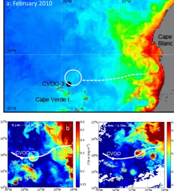
Figure 1. (a)MODIS high resolution chlorophyll picture (4 km2, L3) with the CVOO time-series site (black circle). Satellite chloro- phyll within the ACME is low in February and hard to see (white circle). The pathway of the eddy from the coast to the CVOO site in summer 2009 is indicated by a white dashed line.(b, c)Satel- lite chlorophyll for November/December 2009 and January 2010 (modified, Karstensen et al., 2015). Chlorophyll decreased between November/December 2009 and January 2010, and again between January and February 2010 within the eddy.
in the past as supporting high productivity and chlorophyll standing stock, primarily related to a very shallow mixed layer base in the eddy and the efficiency in vertical trans- port of nutrients into the euphotic zone (McGillicuddy et al., 2007; Karstensen et al., 2016). A comprehensive overview of mesoscale eddies including ACMEs and their physical and biogeochemical linkages is given by Benitez-Nelson and McGillicuddy (2008). Multi-year oxygen time-series data from CVOO show frequent drops in oxygen concentration associated with the passage of ACMEs (Karstensen et al., 2015). One particularly strong event lasted the entire Febru- ary 2010, with lowest oxygen concentrations of only 1–
2 µmol kg−1at about 40 m depth (Karstensen et al., 2015).
Using satellite data, the propagation path of this particular ACME has been reconstructed and found to have formed in summer 2009, at about 18◦N at the West African coast (Fig. 1).
Here we describe particle flux signatures of the passage of this ACME crossing the CVOO in February 2010. We used monthly catches (29-day intervals) from bathypelagic sed- iment traps for the period from December 2009 to March 2011 (Table 1). The total length of the sediment trap data
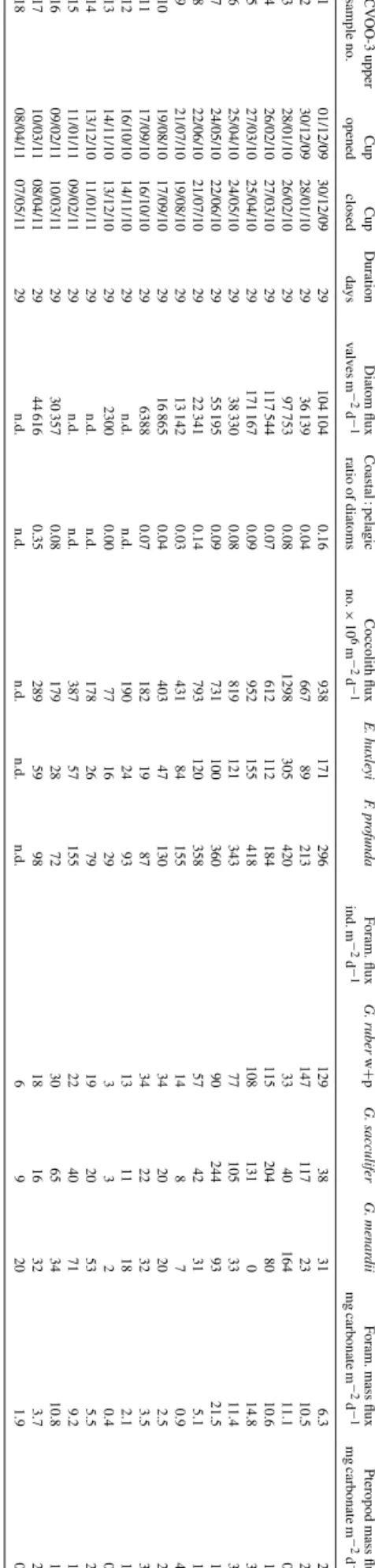
Table1.Collectiondatesfortheupper(1290m)andlower(3439m)traps,bulkmassfluxesandcomposition,molarC:Nratiosoforganicmatterandδ15N(onlylowertrap).Fluxes calculatedfortheentiresamplingperiodsaregiveninitalics. CVOO-3upperCupCupDurationMassfluxesinmgm−2d−1Compositionin%Ratiosδ15N sampleno.openedcloseddaystotalmassBSiOrganiccarbonNitrogenCarbonateLithogenicBSiOrganiccarbonNitrogenCarbonateLithogenicC/Nmolar‰ 101/12/0930/12/092951.242.012.810.3429.5614.053.925.480.6657.6927.429.8 230/12/0928/01/102936.180.461.690.1828.903.431.284.680.5079.889.4810.8 328/01/1026/02/102968.663.116.180.4021.2331.964.539.000.5930.9246.5517.8 426/02/1027/03/102945.763.572.580.2933.503.547.805.630.6373.207.7310.4 527/03/1025/04/102949.580.993.670.4635.545.721.997.410.9371.6711.539.3 625/04/1024/05/102933.170.891.770.2830.640.002.675.340.8492.360.007.4 724/05/1022/06/102953.270.854.100.3942.271.951.607.690.7279.353.6612.4 822/06/1021/07/102927.950.441.760.1822.511.481.576.290.6680.535.3111.2 921/07/1019/08/102914.930.400.780.1413.100.002.695.210.9587.750.006.4 1019/08/1017/09/102914.250.201.160.1910.181.551.398.161.3071.4210.887.3 1117/09/1016/10/102917.630.051.470.2010.194.450.298.341.1257.7925.248.7 1216/10/1014/11/10299.830.090.800.064.933.210.938.130.6350.1732.6415.0 1314/11/1013/12/10296.880.150.730.083.232.032.1710.641.1646.9829.5710.7 1413/12/1011/01/11299.030.110.490.057.210.731.175.440.5579.868.0811.5 1511/01/1109/02/112919.060.171.280.1615.940.390.916.700.8383.622.079.4 1609/02/1110/03/112918.830.221.290.1515.350.681.186.840.7981.533.6010.1 1710/03/1108/04/112917.530.741.490.1710.832.984.248.490.9761.7717.0210.2 1808/04/1107/05/112910.340.340.710.108.930.003.256.891.0086.370.008.1 gm−2per522days15.260.431.010.119.982.272.816.610.7365.3814.8510.6 101/12/0930/12/0929124.974.405.320.5762.5647.363.524.260.4650.0637.9010.94.24 230/12/0928/01/102994.753.103.410.3751.9732.863.273.600.3954.8534.6910.85.21 328/01/1026/02/1029151.0512.5813.310.6321.4090.458.338.810.4214.1759.8824.53.81 426/02/1027/03/1029121.9314.944.630.6361.0436.6912.253.800.5250.0630.098.63.11 527/03/1025/04/102976.173.344.600.4235.2928.344.396.040.5646.3337.2012.73.21 625/04/1024/05/102956.242.822.950.3731.9915.525.015.250.6656.8927.609.33.93 724/05/1022/06/102926.330.511.190.1319.334.111.934.530.4973.4215.6010.83.50 822/06/1021/07/102919.120.430.880.1113.773.152.254.610.5872.0316.499.43.18 921/07/1019/08/102913.390.340.790.098.233.252.535.890.6761.4424.2410.35.35 1019/08/1017/09/102922.380.681.420.1511.307.573.046.330.6750.5033.8111.13.32 1117/09/1016/10/10299.280.240.560.065.232.702.616.010.6056.2929.0711.74.22 1216/10/1014/11/102917.680.391.010.0810.105.172.205.730.4757.1229.2214.33.47 1314/11/1013/12/102919.140.681.230.1610.205.813.546.400.8453.3030.368.96.99 1413/12/1011/01/11297.160.200.370.044.192.022.735.220.5858.6028.2410.54.82 1511/01/1109/02/112910.500.110.640.087.351.751.026.130.7370.0116.729.84.16 1609/02/1110/03/11296.780.110.340.045.680.301.575.090.5283.844.4211.43.42 17–1910/03/1111/05/1162.64.120.160.360.042.320.933.848.660.9156.2822.5511.14.79 gm−1per527days22.791.311.260.1210.588.335.755.530.5146.4136.5512.7
time series of about 16 months allowed us to compare win- ter 2009–2010 with an ACME passage to winter 2010–2011 without an ACME passage in the vicinity of the mooring site.
2 Oceanographic, biological and atmospheric setting at CVOO
The Cape Verde Ocean Observatory (CVOO) is located in the oligotrophic North Atlantic, far west of the coastal upwelling of the Canary Current System (Barton et al., 1998), one of the major eastern boundary upwelling ecosystems (Fréon et al., 2009). A distinct hydrographic boundary exists northwest of CVOO, the Cape Verde Frontal Zone (CVFZ, Zenk et al., 1991), separating the eastern boundary shadow zone with sluggish flow, low oxygen and high nutrient waters from the well-ventilated, high oxygen and nutrient-poorer waters to the west. The different coastal upwelling systems within the Canary Current (CC) have recently been described by Crop- per et al. (2014) with respect to production, phytoplankton standing stock and seasonality.
Monthly maps of surface chlorophyll concentrations de- rived from ocean colour data in the CVOO area showed mostly concentrations below 0.25 mg m−3(Fig. 1). A slight increase in surface chlorophyll was observed during boreal winter months where concentrations of up to 0.5 mg m−3 were found. The high cloud coverage partly prohibits de- tailed analysis of the surface chlorophyll concentrations.
From the few high resolution daily maps available during the CVOO-3 period (Fig. 1), locally enhanced surface chloro- phyll can be identified that coincides with a westward propa- gation of mesoscale eddies, a phenomenon that has been re- ported before (e.g. Benitez-Nelson and McGillicuddy, 2008).
The eddies form in spring and summer at the African coast, in the area between Cape Blanc and Cape Vert, Senegal, and propagate westward at about 5 km per day (Schütte et al., 2016a). Some of the eddies, in particular the ACMEs, ex- hibit low dissolved oxygen (DO) concentrations at very shal- low depth (< 40 m; Karstensen et al., 2015). During CVOO-3, one particular highly productive/low oxygen ACME passed the CVOO site over a period of about 1 month, in February 2010 (Figs. 1 and 3).
The ocean area off West Africa receives the highest supply of dust in the world (Schütz et al., 1981; Goudie and Middle- ton, 2001; Kaufman et al., 2005; Schepanski et al., 2009).
Dust is not only relevant for the climate system (e.g. Ans- mann et al. 2011; Moulin et al., 1997) and the addition of nitrate, phosphate and iron to the surface ocean (e.g. Jick- ells et al., 1998), but also for the ballasting of organic-rich particles (Ittekkot, 1993; Armstrong et al., 2002; Iversen and Ploug, 2010; Ploug et al., 2008; Fischer and Karakas, 2009;
Bressac et al., 2014) formed in the surface ocean. Lithogenic material attributed to mineral dust has been shown to con- tribute between 1/3 and 1/2 to the total deep ocean mass flux off Cape Blanc and south of Cabo Verde (CV-1-2 trap,
ca. 11◦300N, 21◦W; Ratmeyer et al., 1999), respectively.
Typically, mineral dust flux correlates with the satellite- based annual aerosol optical index (Fischer et al., 2010).
High dust fluxes have been found at the oligotrophic EU- MELI site far north of the CVOO (Bory et al., 2001). Fis- cher et al. (2009a) obtained a mean annual lithogenic (dust) flux of 14 g m−2yr−1 for the eastern North Atlantic off West Africa. Seasonality, mass concentrations and long-term chemical characterisation of Saharan dust/aerosols over the Cabo Verde islands based on the Cape Verde Atmospheric Observatory (CVAO) were described by Fomba et al. (2014).
3 Material and methods
3.1 The Cape Verde Ocean Observatory (CVOO) The in situ observations used in this study have been ac- quired at the CVOO, located in the eastern tropical North Atlantic (17◦350N, 24◦150W, Fig. 1) ca. 800 km west of the African coast and about 80 km north of the Cabo Verde is- lands. The site consists of a mooring (3600 m water depth) that was first deployed in September 2006 and has been op- erational since then. The sediment trap data were acquired at two depths during the deployment period October 2009 to May 2011 (CVOO-3). The mooring is equipped with a set of core sensors for hydrography (temperature, salinity sensors at different depth), currents (profiling in the upper 100 m and single rotor current meter (RCM-8) instruments at approxi- mately 600, 1300, and 3400 m depth), and oxygen (typically two single sensors at 50 and 180 m depth). For analysis of the currents, we considered data from one current meter at 588 m, one at 1320 m (30 m below the upper trap), and the deepest at 3473 m (46 m below the lower trap). For the 588 m and the upper trap RCM, complete time series of speed and direction are available. For the lower trap RCM, because of a rotor failure, only current direction but no current speed is available after mid-December 2009. RCM-8 current meters have a speed threshold < 2 cm s−1 and measure speed with
±1 cm s−1 or 2 % of measured speed (whatever is larger).
Speed data < 1.1 cm s−1 have been set to the threshold of 1.1 cm s−1. Compass accuracy is±7.5◦for speed < 5 cm s−1 and 5◦above that threshold.
3.2 Sediment traps and bulk particle flux analyses Particle fluxes were acquired using two cone-shaped and large-aperture sediment traps (0.5 m2; Kiel type; Kremling et al., 1996) at 1290 and 3439 m, respectively. We collected sinking material with bathypelagic traps to circumvent flux biases such as undersampling due to strong ocean currents and/or zooplankton activities (Buesseler et al., 2007; Boyd and Trull, 2007; Berelson, 2002; Yu et al., 2001). We used samples collected on roughly monthly intervals (every 29 days, Table 1). The traps were equipped with 20 cups, which were poisoned with HgCl2before and after deployment by
addition of 1 mL of a saturated HgCl2 solution in distilled water at 20◦C per 100 mL. Pure NaCl was used to increase the density in the cups prior to the deployments (final salinity was 40 ‰). Large swimmers were removed manually and/or by filtering carefully through a 1 mm sieve. Thus, all fluxes refer to the size fraction of < 1 mm. The flux of the size frac- tion of particles > 1 mm was negligible. Samples were wet- split in the home laboratory using a rotating McLANE wet splitter and freeze-dried. Additional method information is given elsewhere (Fischer and Wefer, 1991).
Sediment trap samples were analysed using freeze-dried homogenised material of 1/5 wet splits. It was weighed for total mass and analysed for organic carbon, total nitro- gen, carbonate and biogenic silica. Particulate organic car- bon, total nitrogen and calcium carbonate were measured by combustion with a Vario EL III elemental analyser in the CN mode. Organic carbon was measured after removal of carbonate with 2 N HCl. The overall analytical precision based on internal lab standards was 2.8033±0.0337 % for organic carbon and 0.3187 %±0.0082 for nitrogen, respec- tively. Carbonate was determined by subtracting organic car- bon from total carbon, the latter being measured by combus- tion without pre-treatment with 2 N HCl. Biogenic opal was determined with a sequential 1 M NaOH-leaching method according to Müller and Schneider (1993). The precision of the overall method based on replicate analyses is between
±0.2 and ±0.4 %. Lithogenic fluxes were calculated from total mass flux by subtracting the flux of carbonate, biogenic opal and 2 times the flux of TOC to approximate organic mat- ter. As there is no river input in the study area, we assume that all non-biogenic (=lithogenic) material was supplied via at- mospheric transport.
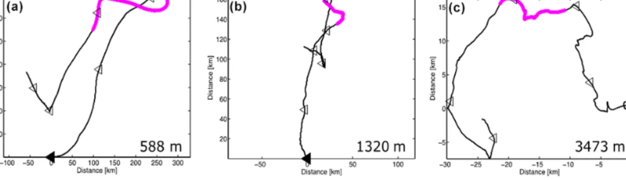
Deep ocean sediment traps collect material from a rather large catchment area, typically around 100 km in diameter or wider, depending on particle settling rates and ocean cur- rents (Siegel and Deuser, 1997). Making use of current meter data records from the upper water column (600 and 1300 m), the progressive vector diagrams (PVDs) showed that the col- lected material before the eddy passage was under the impact of a current from the north-west, while after the eddy pas- sage the material was transported more from the south-west (Fig. 2). In general, the currents were about twice as strong at 600 m compared to the 1300 m depth, and remained mostly below 10 cm s−1.
3.3 Siliceous phytoplankton studies
For this study, 1/125 splits of the original samples were used.
Samples were rinsed with distilled water and prepared for siliceous plankton studies following the method proposed by Schrader and Gersonde (1978). Qualitative and quantitative analyses were done at×1000 magnifications using a Zeiss® Axioscop with phase-contrast illumination (MARUM, Bre- men, Germany). Counts were carried out on permanent slides of acid cleaned material (Mountex®mounting medium). De-
pending on diatom valve abundances in each sample, several traverses across each slide were examined. The total num- ber of counted valves ranged between 300 and 600. At least two cover slips per sample were scanned in this way. Diatom counting of replicate slides indicates that the analytical er- ror of the concentration estimates is≤15 % (Schrader and Gersonde, 1978).
The resulting counts yielded abundance of individual di- atom taxa as well as fluxes of diatom valves per m−2d−1 calculated according to Sancetta and Calvert (1988), as fol- lows:
F =[N] × [A/a] × [V] × [Split] [days] × [D] ,
where [N] is the number of valves, in an area [a], as a frac- tion of the total area of a petri dish [A] and the dilution vol- ume [V] in ml. This value is multiplied by the sample split [Split], representing the fraction of total material in the trap, and is then divided by the number of [days] of sample de- ployment and the trap collection area [D].
3.4 Coccolithophores studies
For coccolith counts, wet split aliquots of each sample (1/25 of the < 1 mm fraction) were further split by means of a rotary sample divider (Fritsch, Laborette 27) using buffered tap wa- ter as the split medium. Studied splits ranged between 1/250 and 1/2500, which were filtered onto polycarbonate mem- brane filters of 0.45 µm pore size. The filters were dried at 40◦C at least for 12 h before a randomly chosen small sec- tion was cut out and fixed on an aluminium stub, sputtered with gold/palladium. The coccolith analysis was carried out using a ZEISS scanning electron microscope at 10 kV accel- erating voltage. In general more than 500 coccoliths were counted on measured transects at a magnification of 3000×. 3.5 Calcareous zooplankton studies
The mass flux of carbonate is mainly constituted of planktonic foraminifera, pteropods and nanofos- sils/coccolithophores. To determine the proportion of calcareous zooplankton, a 1/5 split of the < 1 mm fraction was used to pick planktonic foraminifera and pteropods from the wet solution. The picking was done by hand with a pipette under a ZEISS Stemi 2000 microscope. Picked shells were rinsed three times with freshwater and dried at 50◦C overnight. Total mass fluxes of pteropods and planktonic foraminifera were determined with an analytical balance and mass fluxes (mg m−2day−1) were calculated. The foraminiferal species composition was determined under a ZEISS V8 microscope. The fluxes of all species were given as individuals m−2day−1.
Figure 2.Progressive vector diagram (PVD) of 48 h low pass filtered current meter records at(a)588 m,(b)1320 m, and(c)3473 m for the period from 1 December 2009 (filled triangle at 0.0) to 1 May 2010. The segment in each PVD that corresponds to the ACME passage is indicated by the magenta dots. Open triangles indicate the trap sampling intervals of 29 days. Note, for the deep trap current meter, that the speed failed shortly after installment, and a constant speed of 1.1 cm s−1was used throughout the record.
3.6 Stable nitrogen isotope ratios
For the determination of theδ15N of organic material, about 5 mg of freeze-dried and homogenised material were used.
The δ15N was measured at the ZMT (Leibniz Center of Tropical Marine Ecology, Bremen). The Delta plus mass spectrometer is connected to a Carlo Erba Flash EA 1112 (Thermo Finnigan) elemental analyser via a Finnigan Con- FloII interface. All of the data are expressed in the conven- tional delta (δ)notation, where the isotopic ratio of15N/14N is expressed relative to air, which is defined as zero. The N2 reference gas was research grade and has been calibrated to air using IAEA-N1 and IAEA-N2. The internal standard used was pepton with aδ15N value of 5.73±0.07 % (1σ ).
3.7 Biomarker studies
Freeze-dried and homogenized samples (70–200 mg) were extracted three times with dichloromethane (DCM):
methanol (MeOH) 9 : 1 (v/v) in an ultrasonic bath for 10 min. Internal standards (squalane, 50 ng/nonadecanone, 499.5 ng/ C46-GDGT, 500 ng/erucic acid, 500.5 ng) were added prior to extraction. After centrifugation, solvents were decanted, combined and dried, and saponified (2 h, 80◦C, 1 mL 0.1 M KOH in methanol : water (9 : 1)). Neutral lipids (NLs) were extracted with 4×0.5 mLn-hexane. After acidification to pH < 2 (HCl), fatty acids were recovered with 4×0.5 mL DCM and esterified with methanolic HCl (12 h, 80◦C). Silica-gel chromatography was used to separate NL into hydrocarbons (eluted with n-hexane), aromatic hydro- carbons (n-hexane : DCM, 2 : 1), ketones (DCM : n-hexane, 2 : 1) and polar compounds (DCM : MeOH, 1 : 1).
Alkenones were analysed using a 7890A gas chromato- graph (Agilent Technologies) with a cold on-column (COC) injector, a DB-5MS fused silica capillary column (60 m, ID 250 µm, 0.25 µm film) and a flame ionisation detec- tor (FID). Helium was used as a carrier gas (constant flow, 1.5 mL min−1) and the gas chromatograph (GC) was
heated as follows: 60◦C for 1 min, 20◦C min−1to 150◦C, 6◦C min−1to 320◦C, with final hold time 35 min. Alkenone concentrations were calculated using the response factor of the internal standard (nonadecanone).
U37k0 was calculated as defined by Prahl and Wakeham (1987):
U37k0 = C37:2
(C37:2+C37:3),
and converted to sea surface temperatures (SSTs) using the calibration of Conte et al. (2006).
T (◦C)= −0.957+54.293(U37k0)−52.894(U37k0)2+28.321(U37k0)3 The aromatic as well as fatty acid methyl ester (FAME) frac- tions were analysed by gas chromatography/mass spectrom- etry for the presence of isorenieratene and its derivatives and ladderrane fatty acids.
4 Results 4.1 Mass fluxes
Mass fluxes increased in winter–spring 2009–2010 at both trap depths during the passage of the ACME at CVOO-3, but were rather low in winter–spring 2010–2011 (Fig. 3, Table 1). Fluxes were well correlated between both traps (r2=0.6,N=20), suggesting a fast transfer of the flux sig- nature from the upper water column to bathypelagic depths.
The lower trap fluxes were about twice as high as in the up- per trap during the period of elevated fluxes in winter–spring 2009–2010. During winter 2010–2011, when no large eddy passed the CVOO study site, fluxes showed only a small sea- sonal increase, and the flux to the lower trap was lower in magnitude compared to winter–spring 2009–2010 (Fig. 3).
We consider these to be the “normal conditions”.
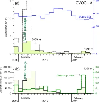
The flux pattern of biogenic silica (BSi) showed a more discrete peak than total mass, with maxima in February–
March 2010 (Fig. 4a). BSi fluxes were highest in March for
0 50 100 150
Total mass flux (mg m-2 d-1)
CVOO - 3
2009 2010 2011
1290 m
february february
3439 m
ACME passage 'normal year'
(winter-spring) without passage of a suboxic eddy pre-
ACME post - ACME
a
c b
Figure 3.Total mass fluxes collected with the upper and lower sed- iment traps at CVOO-3(a). Oxygen time series at approx. 42 m(b) and 170 m(c)water depths (Karstensen et al., 2015); grey bar in- dicates the ACME passage in February 2010. Upper and lower trap fluxes are highly correlated (r2=0.7;N=17); however, lower trap mass fluxes are roughly twice as high during winter–spring 2010 when the ACME passed the site. The common pattern can be seen in winter 2011 during the eddy-free year.
both traps and not in February when the ACME passed the study site. The high BSi fluxes arrived simultaneously at both trap depths without a time/cup lag. BSi fluxes were more than three-fold higher in the lower trap than in the upper trap during February–March 2010 (Fig. 4a). Very low BSi fluxes were measured in winter–spring 2011, and they were slightly higher in the upper trap. On an annual basis, the contribution of BSi to total flux mass was 2.8 % (upper) and 5.75 % (lower trap), respectively. However, during the ACME passage, the contribution increased significantly to 4.5–7.8 % (upper) and 8.3–12.3 % (lower trap) (Table 1). The opal fraction was mainly composed of marine diatoms. Organic carbon fluxes revealed a slightly different pattern from BSi, with one dis- tinct flux peak in February 2010 (Fig. 5a). Organic carbon fluxes in the deep trap were almost twice as high as those
0 5 10 15
BSi flux (mg m-2 d-1)
0 40 000 80 000 120 000 160 000 200 000
Diatom flux (valves m-2 d-1)
0 0.1 0.2 0.3 0.4 0.5
Coastal/pelagic diatom ratio
CVOO - 3
2009 2010 2011
1290 m
F ebruary F ebruary
3439 m
0 20 25 30
SST (°C)
ACME passage
MODIS-SST
2009 2010 2011
F ebruary F ebruary
1290 m
ACME passage
(a)
(b)
Diatom c.p. - ratio
Figure 4. (a)BSi fluxes collected with the upper and lower sedi- ment traps at CVOO-3. During the ACME passage in winter 2010, BSi fluxes were more than 3 times higher in the lower trap. Fluxes in both depth levels were highly correlated (r2=0.9, N=17).
Monthly mean SST from MODIS-Terra-4 km is shown for a 1◦box to the east of the CVOO-3 site (17–18◦N, 23–24◦W).(b)Diatom fluxes and the coastal : pelagic diatom ratio are given for the upper trap samples.
collected in the upper trap during February 2010. In contrast, during the “normal conditions” in winter–spring 2011, or- ganic carbon fluxes showed only minor differences between the upper and lower traps.
Lithogenic (mineral dust) fluxes were more than twice as high in the deep trap during the period influenced by the ACME passage (Fig. 6) and followed organic carbon flux with a distinct peak in February 2010. In particular, the deeper trap samples provided an almost perfect correla- tion between lithogenic material and organic carbon fluxes (r2=0.97,N=17). This correlation was less pronounced but still statistically significant for the upper trap samples (r2=0.63,N=18).
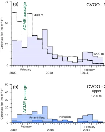
Total carbonate mass fluxes showed less seasonality than BSi and organic carbon, with broad maxima in winter–spring 2009–2010, largely following total mass (Figs. 3, 4, 5, 7).
However, carbonate fluxes showed a decrease in February 2010 during the passage of the ACME, in particular in the deep trap. Fluxes of the major carbonate producers revealed a decrease in pteropod fluxes at both depths during February–
March 2010. Planktonic foraminifera, however, showed a clear flux peak in the deep trap during February 2010 and a rather broad increase in the entire winter–spring 2009–
2010 in the upper trap (Fig. 7b). Total carbonate mass flux in winter–spring 2011 during “normal, non-eddy conditions”
0 5 10 15
Organic carbon flux (mg m-2 d-1)
CVOO - 3
2009 2010 2011
1290 m
february february
3439 m
5 10 15 20 25
C:N molar ratio
3439 m
1290 m
ACME passage
a
b
2 3 4 5 6 7
15NPON (%o) lower trap
0 0.2 0.4 0.6 0.8 1
nitrogen flux (mg m-2 d-1) lower trap
2009 2010 2011
february february
3439 m
c
15N (flux-weighted)
15N
ACME passage
Figure 5.Organic carbon fluxes collected with the upper and lower sediment traps at CVOO-3(a)and the corresponding molar C : N ratios of the organic matter(b). Upper and lower trap fluxes are correlated (r2=0.7,N=17). Note the unusually high C : N ratios in February 2010 recorded in both traps. Typical molar C : N ratios (8–10) for degraded marine organic matter off north-western Africa (Fischer et al., 2003, 2010) are indicated by a green stippled hori- zontal bar in(b)and(c)δ15N values for organic matter sampled by the lower trap (stippled thick line) shown together with the total ni- trogen fluxes. The flux-weighted meanδ15N value of 3.98 is shown as well.
was much lower than in 2010 and decreased between the up- per and lower traps, which is typical for years without eddy passage.
4.2 C/N andδ15N ratios
The molar C : N ratios of the organic material in both traps are rather high for deep ocean material compared to previ- ous findings (Fischer et al., 2003, 2010). In February 2010, C : N ratios were unusually high, with values around 18 and 25 in the upper and lower traps, respectively (Fig. 5b). The δ15N ratios of the lower trap samples varied between 6.99 and 3.11 ‰ (Fig. 5c). The lowest value (3.11 ‰) was mea- sured following the passage of the ACME in February 2010, while the highest value of almost 7 ‰ was recorded in De-
Table2.Fluxesofmajorprimaryandsecondaryproducers/organisms(diatoms,diatomcoastal:pelagicratio,coccolithophoresandplanktonicforaminifera)fortheuppertrapsamples.
CVOO-3upperCupCupDurationDiatomfluxCoastal:pelagicCoccolithfluxE.huxleyiF.profundaForam.fluxG.ruberw+pG.sacculiferG.menardiiForam.massfluxPteropodmassflux
sampleno.openedcloseddaysvalvesm−2d−1ratioofdiatomsno.×106m−2d−1ind.m−2d−1mgcarbonatem−2d−1mgcarbonatem−2d−1
101/12/0930/12/09291041040.1693817129612938316.32.5230/12/0928/01/1029361390.04667892131471172310.52.2328/01/1026/02/1029977530.081298305420334016411.10.9426/02/1027/03/10291175440.076121121841152048010.61.2527/03/1025/04/10291711670.09952155418108131014.83.5625/04/1024/05/1029383300.08819121343771053311.43.6724/05/1022/06/1029551950.09731100360902449321.51.3822/06/1021/07/1029223410.147931203585742315.11.3921/07/1019/08/1029131420.034318415514870.94.21019/08/1017/09/1029168650.04403471303420202.52.01117/09/1016/10/102963880.0718219873422323.53.71216/10/1014/11/1029n.d.n.d.19024931311182.11.91314/11/1013/12/102923000.007716293320.40.81413/12/1011/01/1129n.d.n.d.17826791920535.52.21511/01/1109/02/1129n.d.n.d.387571552240719.21.91609/02/1110/03/1129303570.08179287230653410.81.01710/03/1108/04/1129446160.3528959981816323.72.31808/04/1107/05/1129n.d.n.d.n.d.n.d.n.d.69201.90.4
n.d.:notdetermined
0 25 50 75 100
Lithogenic (= dust) flux (mg m-2 d-1)
CVOO - 3
2009 2010 2011
1290 m
F ebruary F ebruary
3439 m
ACME passage
0 20 40 60 80 100
Dust flux (mg m-2 d-1) 0
5 10 15
Organic carbon flux (mg m-2 d-1)
R²=0.97 N=17
Figure 6.Lithogenic (mineral dust) fluxes collected with the up- per and lower sediment traps at CVOO-3. Upper and lower trap fluxes correspond well (r2=0.83,N=17), but fluxes in the deep trap were more than twice as high compared to the upper trap dur- ing winter–spring when the ACME passed. Note the very close re- lationship with organic carbon (r2=0.97,N=17) shown for the deep trap samples (insert).
cember 2010. Distinct decreases were found from January to March 2010 (ACME passage), as well as from Decem- ber 2010 to March 2011. The mean value was 4.16 ‰, the flux-weighted mean was, at 3.98 ‰, slightly lower. Theδ15N ratios were neither related to the C : N ratios nor to the fluxes of nitrogen and carbon in general.
4.3 Diatom fluxes
The total diatom flux ranged from 2.3×10³ to 1.7×10⁵ valves m−2d−1in the upper trap (Fig. 4b; Table 2). One ma- jor diatom flux maximum (> 1.4×10⁵valves m−2d−1)oc- curred in mid-spring 2010. The opal fraction was mainly composed of marine diatoms. In addition, silicoflagellates, radiolarians, freshwater diatoms, phytoliths and the dinoflag- ellateActiniscus pentasteriasoccurred sporadically. In terms of number of individuals, diatoms dominated the opal frac- tion throughout the year: their flux was always 1 to 4 orders of magnitude higher than the flux of the other siliceous or- ganisms encountered (not shown here). The diverse diatom community was composed of ca. 100 marine species. The most important contributors to the diatom community were species typical of open-ocean, oligo-to-mesotrophic waters of the low- and mid-latitude oceans:Nitzschia sicula,N. bi- capitata,N. interruptestriata,N. capuluspalae, andThalas- sionema nitzschioides var.parva. Resting spores of several coastal species of Chaetoceros, and tycoplanktonic/benthic Delphineis surirella,Neodelphineis indicaandPseudotricer- atium punctatum, are secondary contributors.
0 25 50 75
Carbonate flux (mg m-2 d-1)
CVOO - 3
2009 2010 2011
1290 m
February February
3439 m
ACME passage
0 10 20 30 40 50
Carbonate flux (mg m-2 d-1)
2009 2010 2011
1290 m
February February
Foraminifera Pteropods
ACME passage
(b) (a)
CVOO - 3
upper
Figure 7.Carbonate fluxes collected with the upper and lower sed- iment trap(a)at CVOO-3 shown together with fluxes of planktonic foraminifera and pteropods (only upper trap data,(b), Table 2). Cor- relation of fluxes between both depths is less significant here com- pared to the other bulk components (r2=0.5, n=20). Note that total carbonate fluxes decreased during eddy passage in February 2010.
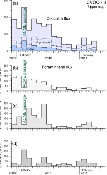
4.4 Coccolith fluxes
In general, both traps revealed coccolith fluxes that were high during the interval December 2009 to May 2010, whereas fluxes were considerably lower (ca. 2–10 times) during the rest of the studied period (Fig. 8a; Table 2). Maximum to- tal coccolith fluxes were recorded in February 2010 for both traps, reaching values of 1300×106coccoliths m−2d−1(up- per trap, Fig. 8a) and 2880×106coccoliths m−2d−1(lower trap, not shown), respectively. Total coccolith fluxes in the lower trap were generally 2–3 times higher than in the up- per trap. In total, 56 coccolithophore species were iden- tified. The coccolithophores were generally dominated by lower photic zone (LPZ) species, such asFlorisphaera pro- fundaandGladiolithus flabellatus, together with more om- nipresent species such asEmiliania huxleyi andGephyro- capsaspp. Florisphaera profundathat constituted between 21.7 and 49.2 % of the total assemblage, and cosmopolitan E. huxleyiranged between 13.4 and 29.4 %. Coccolith fluxes as well as % abundances ofF. profundaslightly decreased in January–March 2010, although this species shows a distinct flux peak in February (Fig. 8a). In contrast, fluxes ofE. hux-
0 500 1000 1500
Coccolith fluxes (no. m-2 d-1)
CVOO - 3
U pper trap
2009 2010 2011
February February
ACME passage
(a)
0 50 100 150 200 250
G. menardii (no. m-2 d-1)
(d)
0 50 100 150 200 250
G. sacculifer (no. m-2 d-1)
(c)
ACME passage
0 50 100 150 200 250
G. ruber , w+p (no. m-2 d-1)
(b)
2009 2010 2011
February February
Coccolith flux
Foraminiferal flux
ACME passage
E. huxleyi
F. profunda
Figure 8.Upper trap fluxes of major primary and secondary car- bonate producing organisms (Table 2).(a)Coccolithophores (total coccolith flux, flux ofE. huxleyiandF. profunda). The planktonic foraminifera(b)G. ruber(white and pink),(c)G. sacculiferand(d) the deep-dwellingG. menardii, the latter showing a distinct peak in flux during the ACME passage in February 2010.
leyias well as their relative proportion clearly increased dur- ing the interval February–March 2010 (Fig. 8a). Other taxa that considerably contributed to the assemblage areGephy- rocapsa ericsonii(2.3–16.7 %),G. oceanica(0.9–6.7 %),G.
muellerae(0.3–14.0 %) andUmbilicosphaera sibogae(1.1–
6.7%), which all show a pattern generally similar to that ofE.
huxleyi. In contrast, deep-dwellingG. flabellatus(1.3–7.3 %) and upper zone speciesUmbellosphaera tenuis(1.3–5.3 %) tend to show less prominent fluxes in February 2010 during the ACME passage. Other, more oligotrophic species (U. ir- regularis,R. clavigera) display a similar pattern.
4.5 Flux of planktonic foraminifera
Planktonic foraminifera showed a clear flux peak in February 2010 in the deep trap (not shown) and a rather broad increase over the entire winter–spring season in 2010 at the upper trap level (Fig. 7b; Table 2). The surface dwellers and warm wa- ter speciesGlobigerinoides ruber white and pink andGlo- bigerinoides sacculiferwere the three dominant species in the total foraminifer flux in both the upper (Fig. 8b, c) and deeper traps throughout. In February 2010, during the pas- sage of the ACME, however, all three species exhibit a de- crease in occurrence. During this interval, they were replaced by the subsurface dwellerGloborotalia menardii, dominating the foraminiferal flux at both trap levels (Fig. 8d, only upper trap shown). The deep dwellers were generally rare at the CVOO-3 site; either they were missing almost completely (Globorotalia truncatulinoides) or they were present in low numbers.Globorotalia crassaformis, for instance, showed a flux pattern with a maximum in April–May in both trap lev- els, following the ACME passage in February 2010.
4.6 Lipid biomarkers
A reduced sample set from the upper trap, covering the sample period from December 2009 to July 2010 (samples 1–8), was used for investigation of the organic biomarker composition and the characterisation of the ACME passage.
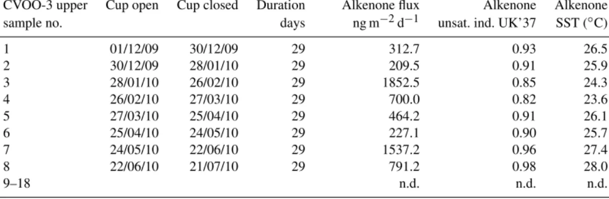
Alkenone-derivedU37k0 values, a biomarker-based proxy for SSTs, varied from 0.82 to 0.98, with the minimum value oc- curring in March, following the ACME passage (Table 3).
Translation of the index into absolute temperatures by using the Conte et al. (2006) global calibration for surface partic- ulate matter resulted in SSTs from 23.6 to 28.0◦C (Fig. 9).
From December 2009 to the end of March 2010, SSTs de- creased from 26.5 to 23.6◦C. After the ACME passage, start- ing in April 2010, SSTs shifted back to around 28.0◦C.
Alkenone fluxes (Fig. 9) showed a distinct six- to eight-fold increase during the ACME passage and correlate with or- ganic carbon flux (Fig. 5a) and the molar C : N ratios of or- ganic matter (Fig. 9,r2=0.77,n=8). The relationship be- tween alkenone and total coccolith fluxes, however, is weak (Figs. 8a and 9). Unique membrane lipids of anammox bac- teria, so-called ladderanes (Sinninghe Damsté et al., 2002) or biomarkers related to a pigment of the photosynthetic green sulfur bacteriaChlorobiaceae, isorenieratene and its deriva- tives, all indicative of photic zone anoxia, could not be de- tected using the analytical tools described above.
5 Discussion
5.1 Production and export within the surface layer of the eddy
The upper CVOO-3 trap revealed a rather unusual high BSi flux in winter–spring (around 4 mg m−2d−1; Fig. 4a) which
Table 3.Fluxes of alkenones, theU37k0-unsaturation index and the estimated SSTs for samples 1–8 of the upper trap.
CVOO-3 upper Cup open Cup closed Duration Alkenone flux Alkenone Alkenone
sample no. days ng m−2d−1 unsat. ind. UK’37 SST (◦C)
1 01/12/09 30/12/09 29 312.7 0.93 26.5
2 30/12/09 28/01/10 29 209.5 0.91 25.9
3 28/01/10 26/02/10 29 1852.5 0.85 24.3
4 26/02/10 27/03/10 29 700.0 0.82 23.6
5 27/03/10 25/04/10 29 464.2 0.91 26.1
6 25/04/10 24/05/10 29 227.1 0.90 25.7
7 24/05/10 22/06/10 29 1537.2 0.96 27.4
8 22/06/10 21/07/10 29 791.2 0.98 28.0
9–18 n.d. n.d. n.d.
n.d.: not determined
was partly higher than at the more coastal and mesotrophic Cape Blanc site CB (Fischer et al., 2003). The latter site is located within the Giant Cape Blanc filament and is charac- terised by high chlorophyll streaming offshore (Van Camp et al., 1991; Helmke et al., 2005). We argue that the un- usually high BSi flux during the eddy passage was due to diatom production within the surface waters of the ACME.
The diatom flux pattern revealed a distinct increase in Febru- ary 2010, with a major peak later in early spring (Fig. 4b).
The base of the mixed layer that coincides with the nutri- cline (Karstensen et al., 2016) shoaled from about 50–60 m before (and after) the eddy passage to about 20 m during the eddy passage (Karstensen et al., 2015). Elevated chlorophyll within the eddy is seen (Fig. 1) and has been discussed in the context of upward nutrient fluxes into the euphotic zone, particularly associated with ACMEs (e.g. Karstensen et al., 2015; Benitez-Nelson and McGillicuddy, 2008). Consider- ing the timing of the distinct BSi and diatom flux signals, this may indicate that the organic carbon is primarily fixed on the western side of the eddy where an intense bloom is expected (Chelton et al., 2011). Sargasso Sea ACMEs, for instance, contain significant numbers of diatoms, regardless of the age of the eddy (McNeil et al., 1999; Sweeney et al., 2003; Ewart et al., 2008).
The molar C : N ratios of organic matter were unusually high in February 2010 for both trap depths (Fig. 5b). They clearly fall far off the range of deep-ocean sediment trap sam- ples or surface sediments with partly degraded organic ma- rine material (C : N around 8–10; Fischer et al., 2003, 2010;
C : N=5–10, Tyson, 1995; Wagner and Dupont, 1999). The exceptionally high ratios in February 2010 (C : N=18 (up- per) and 25 (lower trap)) (Fig. 5b), however, cannot be ex- plained by mixing processes of marine (C : N around the Redfield ratio, Redfield et al., 1963; Martiny et al., 2013) and terrestrial organic materials (C : N global mean=24, Ro- mankevich, 1984), because this would imply a preferential contribution of terrestrial organic matter. On the one hand, nitrogen (nitrate) limitation in the surface water north of
0 1000 2000 3000
Alkenone flux (ng m-2 d-1)
CVOO - 3
Upper trap
2009 2010
F ebruary F ebruary
0 20 25 30
SST (°C)
ACME passage
SST (UK'-37 index)
MODIS-SST
L ipids not determined
4 8 12 16 20
Molar C:N ratio 0
500 1000 1500 2000
Alkenone flux
r²=0.77 N = 8
2011
Figure 9.Alkenone fluxes together with theU37k0-derived and satel- lite SSTs, for the time period before and after the ACME passage.
Molar C : N ratios taken from Fig. 5b, which correlate well with the alkenone fluxes, are shown in the insert (r2=0.77,N=8).
the Cabo Verde islands combined with low growth rates of the primary producers (both diatoms and coccolithophores) would explain the elevated C : N ratios of organic matter (e.g.
Laws and Bannister, 1980; Martiny et al., 2013; Löscher et al., 2015a). However, since oxygen : nitrate ratios are about twice as high in the eddy compared to the surrounding wa- ters, enhanced nitrogen recycling could explain the extraor- dinarily high C : N ratios as well (Karstensen et al., 2016).
Nitrogen limitation is also known to increase the C : N ra- tios of the alkenone producers (e.g. Loebl et al., 2010), and might result in an increase in the production and storage of alkenones (e.g. Eltgroth et al., 2005; Prahl et al., 2003).
Alkenone temperature records from the Subtropical Front at the Chatham Rise, south-western Pacific Ocean (Sikes et al., 2005), showed that biases occurred during times of highest lipid fluxes and low nutrient conditions in the surface mixed layer. When plotting the C : N ratios vs. the alkenone fluxes of the upper trap samples, we indeed obtain a relationship (Fig. 9,r2=0.77,n=8) which points to nutrient limitation