Models for Neutrino Masses and Mixings

Nuclear Physics B Proceedings Supplement 00 (2021) 1–8

Proceedings Supplement

Models for Neutrino Masses and Mixings

Stefan Antusch^a,b

aDepartment of Physics, University of Basel, Switzerland

bMax-Planck-Institut f¨ur Physik (Werner-Heisenberg-Institut), M¨unchen, Germany

Abstract

We review recent developments towards models for neutrino masses and mixings.

Keywords: Neutrinos, fermion masses and mixings

1. Introduction

The last year has been an exciting time for mod- els of neutrino masses and mixings, especially due to the recent measurement of the leptonic mixing angle θ₁₃^PMNS by T2K [1], DoubleCHOOZ [2], DayaBay [3]

and RENO [4], featuring

θ^PMNS₁₃ =8.8^◦±1.0^◦. (1) This rather accurate measurement has dramatic conse- quences for model building. Out of the many models proposed, a large fraction is now excluded and only a small fraction remains which can explain the experi- mentally found value.

One might now think that theorists get depressed by so many models being ruled out, however of course just the opposite is true: The measurement has triggered an enormous interest in the community and a large number of theory papers appeared, analysing its consequences.

Another reason why this field is so lively is the fact that there are still many unknowns in the neutrino sec- tor, which means that models still have the possibility to make predictions. In this respect, the measured value of θ₁₃^PMNScan now be used as an input parameter for build- ing models to predict these currently unknow parame- ters, such as, e.g.,

• the Dirac CP phaseδ^PMNS,

• the deviation ofθ₂₃^PMNSfrom maximal mixing,

• the neutrino mass ordering (normal or inverse),

• the neutrino mass scale,

• whether neutrino masses are of Dirac- or Majorana-type,

• and if neutrinos have Majorana masses, the values of the Majorana CP phases.

2. The Neutrino Puzzles

There are two main puzzles in the neutrino sector:

The first one may be called the “mass puzzle”. It sum- marises the challenge to find the right extension of the Standard Model (SM) giving rise to the observed neu- trino masses and to explain their smallness. The second one may be called the “neutrino flavour puzzle”, con- taining the question of why the leptonic mixing angles are large compared to the quark mixing angles of the CKM matrix, and whether there is any pattern hidden in the leptonic mixing angles that could guide us towards the theory of flavour (where we still have a long way to go).

2.1. The Mass Puzzle

As you all know, various mechanisms have been pro- posed to introduce masses for the neutrinos. For exam- ple, there are the well-known tree-level possibilites, the seesaw mechanisms (of type I [5], type II [6] and type III [7]). But there are also proposals where, for exam- ple, neutrino masses emerge only at loop level, or from non-perturbative effects in string theory.

arXiv:1301.5511v1 [hep-ph] 23 Jan 2013

Many models leading to Majorana neutrino masses can, at low energies relevant for neutrino oscillation physics, be described by the SM plus a dimension five neutrino mass operator [8] and eventually plus higher- dimensional operators leading, e.g., to a non-unitarity of the leptonic mixing matrix [9]. However, neutri- nos may also be Dirac particles, with the smallness of the masses explained, e.g., in extra-dimensional theo- ries from a small overlap of the neutrino wave-functions with the four-dimensional brane where the SM fields are confined to [10, 11]. And finally, it may well be that the true mechanism realized in nature has not been pro- posed yet.

The present status is that there are no experimental hints to tell us which of the proposed mechanisms (if any) is the right one. It is not even known at which scale neutrino masses are generated. While many mod- els based on a seesaw mechanism assume neutrino mass generation at very high energies (close to the GUT scale M_GUT ∼10¹⁶GeV), the small neutrino masses can also be generated at energies around the TeV scale, or even at much lower energies such that light sterile neutrinos can propagate in oscillation experiments.

To make progress towards this question, it will be necessary to combine all experimental data which will be available in the future, i.e. from the LHC, from indi- rect tests (for example from charged lepton flavour vio- lation searches and tests of the non-unitarity ofUPMNS) as well as from experiments on the type and value of the absolute neutrino mass scale (from cosmology, Tritium β-decay, 0νββ-decay) and from neutrino oscillation ex- periments.

2.2. The Neutrino Flavour Puzzle

The “neutrino flavour puzzle”, i.e. the puzzle of why the leptonic mixing angles are large compared to the quark mixing angles of the CKM matrix, and whether there is any pattern hidden in the leptonic mixing an- gles, will be the main part of my talk. Let us start by briefly reviewing the present knowledge of quark and lepton masses and mixings, which is summarized in ta- ble 1. Regarding the mixing angles, it is indeed strik- ing that they are large in the lepton sector, while the largest mixing angle in the quark sector, the Cabibbo angle θ_C ≡ θ^CKM₁₂ ≈ 13.0^◦, is of the same order as the recently measured smallest leptonic mixing angle θ₁₃^PMNS≈9^◦±1^◦. CP violation in the CKM matrix is pa- rameterized by a large Dirac CP phase,δ^CKM≈69^◦±3^◦, while the CP phase(s) in the neutrino sector are still un- known.

Regarding the masses, we see that in the quark and charged lepton sectors, there is a strong hierarchy be-

Quark and lepton mixing angles:

θ₁₂^PMNS≈34^◦±1^◦ θ^CKM₁₂ ≈13.0^◦ θ₂₃^PMNS≈46^◦±3^◦ θ^CKM₂₃ ≈2.4^◦ θ₁₃^PMNS≈9^◦±1^◦ θ^CKM₁₃ ≈0.2^◦ δ^PMNSunknown δ^CKM≈69^◦±3^◦

Quark masses (atµ=mt):

mu≈0.0012 GeV md≈0.0028 GeV mc≈0.590 GeV ms≈0.052 GeV mt≈162.9 GeV mb≈2.8 GeV

Lepton masses:

|m²₃−m²₁| ≈2.4×10⁻³eV² me≈0.0005 GeV m²₂−m²₁≈7.6×10⁻⁵eV² mµ≈0.0102 GeV

mi<O(0.5 eV) mτ≈1.8 GeV

Table 1: Overview over the present knowledge of quark and lepton masses. For quarks and charged leptons, the running masses at the top mass scale,µ=m_t(mt) are given [12]. The neutrino results are based on the global fit from [13]. Hints forθ^PMNS₂₃ <45^◦have been reported in [14].

tween the masses of the three families. This hierarchy is strongest in the up-type quark sector, while the masses are less hierarchical in the down-type quark and charged lepton sectors, and similar for each family of down-type quarks and charged leptons. This similarity may be a consequence of Grand Unified Theories (GUTs). We will come back to this possibility in the context of mod- els for large θ^PMNS₁₃ later in my talk. Of course in the neutrino sector only two mass splittings are known and the absolute neutrino mass scale is only constrained to be (roughly) below 0.5 eV from cosmology, Tritiumβ- decay and 0νββ-decay experiments.

3. Ideas and Approaches

3.1. Top-down Approaches

There are various ways to approach the above- mentioned neutrino puzzles. Possible top-down view- points are, for example:

• Anarchy:In anarchy [15], the idea is that the large mixing in the lepton sector is the result of a lack of structure. When the neutrino mass matrix is filled with random entries, it is indeed plausible that the resulting mixing angles are large. In fact, ifθ^PMNS₁₃ would have been very small, this would have been an argument against this viewpoint. With the now measured not so small value, this idea is still alive.

However, it is also hard to test since only proba- bilities are predicted, but not specific values of pa- rameters, which can be tested in experiments.

• Family symmetries: Here the approach is to ex- plain the neutrino mixing properties by assuming additional structure, generated by additional sym- metries beyond the gauge symmetries of the SM.

To generate flavour structure, such symmetries dis- tinguish between members of different families.

They are therefore called family symmetries or horizontal symmetries. Such symmetries can, on the one hand, explain the hierarchy of the masses in the quark and charged lepton sectors [16], but they can also explain the large mixing in the lepton sec- tor. Non-Abelian discrete symmetry groups, like e.g.A4orS4, have become very popular in this re- spect [17].

• Grand Unified Theories (GUTs): In GUTs [18, 19], the forces of the SM can be unified at high energies, aroundM_GUT =2×10¹⁶GeV. Left-right- symmetric GUTs are also appealing because they predict small neutrino masses via a version of the seesaw mechanism. In general, GUTs not only unify the forces of the SM, but also different types of particles are unified in joint representations of the GUT symmetry group. This GUT symmetry group contains the SM gauge group as a subgroup and, compared to family symmetries, it acts “verti- cally”. This means it is linking properties of differ- ent particle types, such that the flavour structures of quarks and leptons are no longer disconnected.

• Extra Dimensions and String Theory: Alterna- tively, one may also attempt to approach the neu- trino puzzles directly from extra-dimensional the- ories or from the perspective of string theory. As already mentioned, one approach to explain the smallness of Dirac-type neutrino masses uses a small overlap of the neutrinos wave-function with our four-dimensional brane [10, 11]. In another approach, for instance, neutrino masses and large lepton mixing emerge from string theory instanton effects [20, 21].

3.2. Bottom-up Suggestions

In addition, there have been various suggestions for relations between mixing parameters, inspired by bottom-up considerations based on the improved accu- racy of the experimental data. Suggested relations of this type are, e.g.:

• Tri-bimaximal mixing:Tri-bimaximal (TB) mix- ing [22] is a specific mixing pattern, defined by

θ₁₂^PMNS=arcsin 1

√ 3

!

, θ^PMNS₂₃ =45^◦, θ^PMNS₁₃ =0^◦. (2) Before the measurement ofθ^PMNS₁₃ , it was in excel- lent agreement with the experimental data. With its predictionθ^PMNS₁₃ =0^◦, it is now known that TB mixing can not hold exactly. However, as we will discuss later, it may still be a viable leading order structure of the neutrino mixing matrix.

• Bimaximal mixing:The bimaximal (BM) mixing pattern [23] was proposed earlier than TB mixing, and is defined by

θ^PMNS₁₂ =45^◦, θ₂₃^PMNS=45^◦, θ₁₃^PMNS=0^◦. (3) Of course,θ^PMNS₁₃ as well asθ^PMNS₁₂ have to be cor- rected, compared to the BM prediction, in order to be consistent with the present experimental data.

• Quark-lepton complementarity: Quark-lepton complementarity (QLC) suggests a link between the quark and lepton mixing angles of the form

θ^PMNS₁₂ +θ_C=45^◦, (4) which is called the QLC relation [24]. It was discussed that this relation (and other similar re- lations) may be obtained by multiplying a bi- maximal mixing matrix times a mixing matrix equal to the CKM matrix [24, 26].

• Finally, in the light of the recent measurement of θ^PMNS₁₃ =8.8^◦±1.0^◦, which is consistent with

θ₁₃^PMNS= θC

√

2 , (5)

it has been suggested that this value ofθ^PMNS₁₃ may be a footprint of an underlying GUT, and it has been discussed that it can indeed emerge as a (lead- ing order) prediction in realistic GUT models under simple conditions[25].¹

One main theme in the last years has been to try to connect bottom-up suggestions to model building ap- proaches following the various top-down viewpoints. In my talk, I will now discuss two examples, and I apolo- gize if I can not cover your favourite topic (due to lack of time, respectively space).

1In the context of some versions of QLC, where a bi-maximal mix- ing matrix is multiplied with a matrix equal to the CKM matrix in a certain way, the relation of Eq. (5) has been mentioned in [26]. Re- cently, a modification of the TB mixing scheme with this value of θ^PMNS₁₃ (with unchangedθ₁₂^PMNSandθ^PMNS₂₃ ) has been suggested in [27].

4. Family Symmetries and Mixing Patterns

One aspect, which received a lot of attention in the last years, is the possibility to realize specific neutrino mixing patterns, in particular TB mixing, with the help of family symmetries like, for instance, A4 andS4. In model-building, one may distinguish two possibilities, which may be called (following [28]) direct models and indirect models. For the following discussion we will focus on the example of TB mixing, where the leptonic mixing matrix takes the special form [22]

UTB=















 q2

3

√1

3 0

−√¹ 6

√1 3

√1 1 2

√ 6 −√¹

3

√1 2

















. (6)

leading to the TB pattern of mixing angles in Eq. (2).

4.1. Preliminary Remark: Symmetries which enforce TB Mixing are Broken Symmetries

How can family symmetries be related to mixing pat- terns like TB mixing? The first idea could be that there might be a symmetry which one just has to impose on the theory (as an unbroken exact symmetry) and which would then force the mixing to TB form. One can easily see that this is not possible.

If such a symmetry would exist for the whole the- ory, then one consequence would be that the mixing pattern is stable under renormalization group (RG) run- ning. However, one can show that this is not the case. It therefore follows that no unbroken symmetry can exist to enforce TB mixing. Of course this is not the end of the story, as I will explain in the next two subsections, however one should keep in mind that we are talking about broken family symmetries.

Let us discuss the RG running effects in a bit more detail: Below the seesaw scales, i.e. the masses of the right-handed neutrinos in type I seesaw models, and up toO(θ13) corrections, the evolution of the mixing angles is given by [29] (dropping here the PMNS labels for the mixing parameters for brevity)

θ˙₁₂ = −Cey²_τ

32π² sin 2θ₁₂s²₂₃|m1e^iϕ1+m2e^iϕ2|²

∆m²₂₁ , (7) θ˙₁₃ = Cey²_τ

32π² sin 2θ₁₂ sin 2θ₂₃ m3

∆m²₃₁(1+ζ)

×I(mi, ϕi, δ), (8) θ˙23 = −Cey²_τ

32π²

sin 2θ23

∆m²₃₁

hc²₁₂|m2e^iϕ2+m3|²

+s²₁₂ |m1e^iϕ1+m3|² 1+ζ

#

. (9)

The dot indicates differentiation d/dt ≡ µd/dµ (with µbeing the renormalization scale), and the abreviations s_{i j} = sinθ_{i j}, c_{i j} = cosθ_{i j}, ζ = ∆m²₂₁/∆m²₃₁ (with the mass squared differences∆m²_{i j}=m²_i −m²_j) and

I(mi, ϕi, δ)=m1cos(ϕ1−δ)

−(1+ζ)m2cos(ϕ2−δ)−ζm3cosδ (10) have been used. In the SM, Ce = −3/2, while in the MSSM,Ce = 1. yτdenotes the tau Yukawa coupling, and one can safely neglect the contributions coming from the electron and muon Yukawa couplings. For the Majorana phasesϕ1andϕ2, we use the same convention as in [29].

From these expressions one can easily estimate the typical size of RG effects on the leptonic mixing angles and see some basic properties. In particular, one can see that TB mixing is not stable under RG running.² 4.2. TB Mixing in Direct Models

Despite the fact that family symmetries for TB mix- ing have to be broken, there is still hope to identify use- ful underlying family symmetries and to apply them for realizing the TB mixing pattern. In direct models, the idea is to make use of remnant symmetries in the neu- trino and the charged lepton sectors. If an underlying family symmetry groupGF had existed (and was then spontaneously broken) such remnant symmetries might have survived, and by identifying them one could at least recover part of GF. Such considerations lead to the family symmetry group S4 [31] or closely related groups as the minimal possibilities forGF.³

For instance, assuming TB mixing and working in the neutrino flavour basis, one finds that the generatorsS andU(for definitions, see, e.g., [28]) are preserved in the neutrino sector, while the diagonal generator T is preserved in the charged lepton sector. Combining them one arrives at the symmetry groupS₄. Now engineering backwards, one can make sure that a model generates TB mixing if one first postulates a symmetry groupG_F containingS4and then breaks it spontaneously such that the symmetries generated byS,U respectivelyT sur- vive in the neutrino and charged lepton sectors as rem- nant symmetries.

2Analytical formulae including the effects of the neutrino Yukawa couplings, relevant above the mass thresholds of the right-handed neu- trinos, can be found in [30].

3We note that alsoA₄is suitable for constructing direct models with TB mixing, if only part of the available group representations are used.

4.3. TB Mixing in Indirect Models

While in direct models the symmetry group plays the central role, the key feature of indirect models are the directions in flavour space in which the family symme- try is broken. In fact, if the symmetry groupGF is bro- ken along the directions given by the columns of the TB mixing matrixU_TB of Eq. (6), then TB mixing in the neutrino sector can easily be realised, independent of the neutrino mass eigenvalues. This can be used in model building by promoting the columns of UTB to dynamical fields, the so-called flavons, and by making their vacuum expectation values point in the desired di- rections in flavour space.⁴

Although here the choice of the symmetry group is not as crucial as in direct models, it has turned out that for making the flavons align in the right directions, non-Abelian discrete symmetries (like A4 or S4) are favourable. In the recent years, various models have been constructed by many authors following the direct or indirect approach, and using non-Abelian discrete groups as family symmetryGF.

4.4. TB Mixing Confronted with Recentθ₁₃^PMNSResults As we have already stated above, exact TB mixing (which features zero θ^PMNS₁₃ ) is ruled out by the latest experimental results forθ^PMNS₁₃ . Model builders show two possible reactions w.r.t. this fact:

• One possible reaction is togive up TB mixing and to look for alternative structureswhich already feature non-zero largeθ^PMNS₁₃ . Within the direct ap- proach to model building, this could for example imply to use different discrete symmetry groups, as e.g. in [33]. In the context of indirect models, such structures can arise from breaking the familly groupGF along a new direction in flavour space, as e.g. in CSD2 [34] which leads to so-called tri- maximal mixing with predicted value ofθ^PMNS₁₃ .

• Another possible reaction is toview TB mixing as a leading order pattern only, and to apply correc- tions to it. Such corrections could, for example, be applied to the family symmetry breaking vacuum expectation values of the flavon fields [35]. An- other, quite popular and in fact very well motivated correction is provided by charged lepton mixing contributions (see e.g. [36]), as we will discuss in more detail in the following section.

4We note that this concept may easily be applied in seesaw mod- els, but it can also be used in other scenarios, e.g. in the context of string theory models where the neutrino masses emerge from instan- ton effects [21]. In seesaw scenarios, it is called form dominance [32].

Y

Y

Y

m

UPMNS=U^e†U^ν UCKM=U^u†U^d

GUTrelations

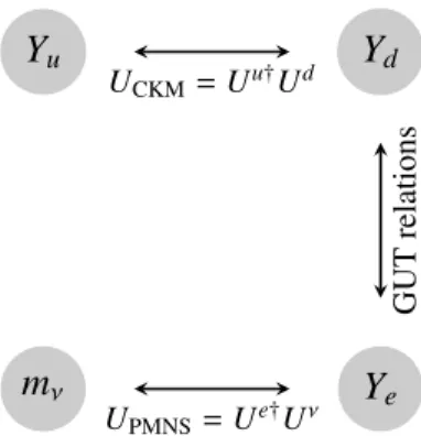
Figure 1: Using GUT relations between the down-type quark and charged lepton Yukawa matrices, and some simple conditions, charged lepton mixing effects can induceθ^PMNS₁₃ ≈θC/√

2 in GUT models.

5. θ^PMNS

13 from charged lepton mixing effects - are there GUT footprints in the PMNS matrix?

In GUT models of flavour, non-zeroθ^PMNS₁₃ is gener- ically expected due to the presence of charged lepton mixing contributions. The general picture is illustrated in Fig. 1. The quark mixing matrix is composed from the left diagonalization matrices of the down-type and up-type quark mass matrices (or of the corresponding Yukawa matricesYdandYu),UCKM=U^u†U^d, and anal- ogously the lepton mixing matrix is composed from the left diagonalization matrices of the neutrino mass ma- trixmνand of the charged lepton Yukawa matrixYe, i.e.

UPMNS=U^e†U^ν.

In GUTs, quarks and leptons are unified in joint rep- resentations of the GUT symmetry group, which im- plies that the elements of the quark and lepton Yukawa matrices can arise (dominantly) from single joint oper- ators. As a consequence, the flavour structures of the quark and the lepton sectors are linked and Yd andYe

are connected via “GUT relations”. Under some simple conditions, these GUT relations can lead to predictive schemes for θ^PMNS₁₃ , which may appear as “footprints”

of GUTs in the PMNS matrix, as we will discuss be- low. One possible footprint is the phenomenologically attractive relationθ^PMNS₁₃ ≈θC/√

2.

5.1. θ^PMNS₁₃ ≈θ_C/√

2from GUTs

Let us now discuss, following [25], how predictions forθ^PMNS₁₃ , linked to the Cabibbo angle of the quark mix- ing matrix, can arise in GUT models:

• Our starting point is the neutrino mass matrix. Let us consider the case that the 1-3 mixing in the neu- trino sector (here referred to asθ^ν₁₃) is negligibly

small,

θ^ν₁₃≈0, (11)

as it holds true, for example, in TB neutrino mixing and bimaximal neutrino mixing.

• Turning to the quark sector, we can see from Tab. 1 that the hierarchy between the masses of the three families is stronger in the up-type quark sector than in the down-type quark sector. With hierarchical mass matrices, the stronger hierarchy is generically associated with the smaller mixing, such that we often encounterθ_{i j}^u θ^d_{i j}, leading to

θ^d₁₂ ≈θC , (12) while the other mixing angles in Yd are much smaller than the Cabibbo angle and will be ne- glected in the following discussion.

• As mentioned above, GUT relations connect quark and lepton masses, when the elements of the quark and lepton Yukawa matrices arise dominantly from single joint GUT operators. In an analogous fash- ion, this also leads to relations between quark and lepton mixing angles. In particular, the 1-2 mix- ings inYeandYd are then connected by ratios of Clebsch factorsci j, for example by [38, 39]⁵

θ^e₁₂≈ c12

c22

θ^d₁₂≈ c12

c22

θC, (13)

where Eq. (12) has been used in the last step.

• Finally, recalling thatθ^ν₁₃ ≈0 (and that alsoθ^e₁₃ is negligibly small), one finds that the charged lepton mixing contributionθ^e₁₂(viaUPMNS=U^e†U^ν) now determinesθ^PMNS₁₃ . In addition,θ^e₁₂also changes the solar mixing angleθ^PMNS₁₂ , as we will discuss in the next subsection. The inducedθ^PMNS₁₃ is given by

θ₁₃^PMNS≈θ₁₂^e s^PMNS₂₃ ≈ θ^e₁₂

√ 2

≈ θ_C

√ 2

c₁₂ c22

, (14)

where in the second step a maximal mixingθ^PMNS₂₃ has been plugged in, and in the third step the ”GUT mixing relation” Eq. (13) has been used. One can see thatθ^PMNS₁₃ is predicted in terms of the Cabibbo

5Available Clebsch factors in SU(5) GUTs are, e.g., {¹₂,1,³₂,3,⁹₂,6,9} and in Pati-Salam models, e.g., {³₄,1,2,3,9}.

For the corresponding GUT operators and their viability in supersym- metric scenarios, see e.g. [37].

-180 ° -90 ° 0 ° 90 ° 180 °

20 ° 25 ° 30 ° 35 ° 40 ° 45 ° 50 °

∆^PMNS Θ12Ν

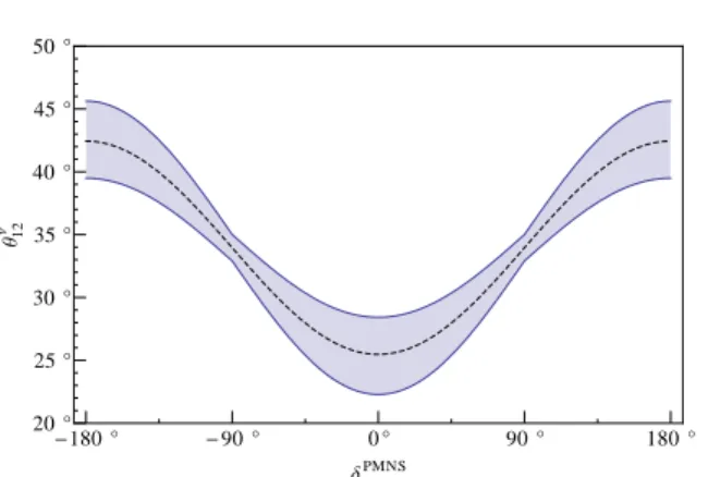
Figure 2: Using the lepton mixing sum rule of Eq. (15), a measure- ment ofδ^PMNSallows to reconstructθ₁₂^ν (provided thatθ^ν₁₃,θ^e₁₃θ_C).

The shaded region corresponds to the present 1σuncertainties for θ^PMNS₁₂ ,θ^PMNS₁₃ andθ^PMNS₂₃ , using the version of the sum rule with gen- eralθ^PMNS₂₃ [36, 41]. The figure is taken from [25].

angle times a ratio of Clebsch factors.⁶ The spe- cific relation θ^PMNS₁₃ ≈ θC/√

2 arises when two Clebsch factors are set equal.⁷

5.2. The Lepton Mixing Sum Rule

In the scenario described in the previous subsection, the charged lepton mixing contributionθ^e₁₃ also modi- fies the 1-2 mixing ofU^ν according toθ^PMNS₁₂ ≈ θ^ν₁₂ +

θ^e₁₂

√

2cos(δ^PMNS), assuming maximalθ^PMNS₂₃ here for sim- plicity. Using Eq. (14), one obtains the following rela- tion,

θ^PMNS₁₂ −θ^PMNS₁₃ cos(δ^PMNS)≈θ^ν₁₂ , (15) known as the lepton mixing sum rule [36, 41].

With a future measurement ofδ^PMNS, the lepton mix- ing sum rule can be used to test whether a special mix- ing pattern, like e.g. TB mixing or bimaximal mixing, is realized in the neutrino sector. This is illustrated in Fig. 2. TB neutrino mixing, for example, would corre- spond toθ^ν₁₂ =arcsin(1/√

3) ≈35.3^◦ and can only be viable forδ^PMNS ≈ ±90^◦, whereas bimaximal neutrino mixing withθ₁₂^ν =45^◦requiresδ^PMNS≈180^◦.⁸

6It should be noted in this context that many existing GUT models have predicted smaller values ofθ^PMNS₁₃ (often around 3^◦), especially when they were using the Georgi-Jarlskog Clebsch factor of 3 to ob- tain viable mass relations for the second and the first quark and lepton families [40].

7We note that the conditions are somewhat different in SU(5) GUTs and in Pati-Salam unified models. Details are left out here for brevity and can be found in [25].

8Such specific predictions forδ^PMNS may emerge from flavour models withZ2orZ4shaping symmetries to explain a right-angled CKM unitarity triangle (withα≈90^◦), as discussed recently in [42].

6. Summary and Conclusions

The recent measurement ofθ^PMNS₁₃ = 8.8^◦±1.0^◦ is exciting news for model building. A large fraction of the proposed models are now ruled out, and new ideas are being developed towards explaining the experimentally found value.

While exact mixing patterns with vanishing θ₁₃^PMNS, like for example TB mixing ofU_PMNS, are ruled out, they may still provide viable leading order structures.

Especially when mixing patterns are realized in the neu- trino sector, withθ^PMNS₁₃ originating from charged lep- ton 1-2 mixing contributions, this can lead to alternative scenarios with high predictivity.

Independent of such neutrino mixing patterns, it is in- teresting that the phenomenologically attractive relation θ₁₃^PMNS≈θC/√

2 can be a consequence of an underlying Grand Unified Theory.

After this great experimental success of measuring θ₁₃^PMNS, the next goals will include the measurement of the neutrino mass ordering, the Dirac CP phaseδ^PMNS, and the deviation ofθ^PMNS₂₃ from maximal mixing. In addition,θ^PMNS₁₃ will be measured even more precisely, with an accuracy goal of about±0.25^◦. The results of these measurements will provide the next crucial input for model building.

Finally, I would like to note that given the (already present) high experimental precision for the leptonic mixing parameters, it is important that also the theoreti- cal analyses of models for neutrino masses and mixings are performed with comparable accuracy.

Acknowledgments

I would like to thank the organizers of Neutrino 2012 for their effort to make this great conference possible.

Furthermore, I want to thank the Swiss National Science Foundation for support.

References

[1] K. Abeet al.[T2K Collaboration], Phys. Rev. Lett.107(2011) 041801 [arXiv:1106.2822 [hep-ex]].

[2] Y. Abeet al.[DOUBLE-CHOOZ Collaboration], Phys. Rev.

Lett.108(2012) 131801 [arXiv:1112.6353 [hep-ex]].

[3] F. P. Anet al.[DAYA-BAY Collaboration], Phys. Rev. Lett.108 (2012) 171803 [arXiv:1203.1669 [hep-ex]].

[4] J. K. Ahnet al.[RENO Collaboration], arXiv:1204.0626.

[5] P. Minkowski, Phys. Lett. B67(1977) 421; T. Yanagida inProc.

of the Workshop on Unified Theory and Baryon Number of the Universe, KEK, Japan, 1979; S.L. Glashow, Cargese Lectures (1979); M. Gell-Mann, P. Ramond and R. Slansky in Sanibel Talk, CALT-68-709, Feb 1979, and inSupergravity(North Hol- land, Amsterdam 1979); R. N. Mohapatra and G. Senjanovic, Phys. Rev. Lett.44(1980) 912.

[6] M. Magg and C. Wetterich, Phys. Lett. B 94 (1980) 61;

J. Schechter and J. W. F. Valle, Phys. Rev. D 22 (1980) 2227;

G. Lazarides, Q. Shafi and C. Wetterich, Nucl. Phys. B181 (1981) 287; R. N. Mohapatra and G. Senjanovi´c, Phys. Rev.D23 (1981), 165; C. Wetterich, Nucl. Phys.B187(1981), 343.

[7] R. Foot, H. Lew, X.-G. He and G. C. Joshi, Z. Phys. C44 (1989) 441. E. Ma, Phys. Rev. Lett.81(1998) 1171; E. Ma and D. P. Roy, Nucl. Phys. B644, 290 (2002); T. Hambye, L. Yin, A. Notari, M. Papucci and A. Strumia, Nucl. Phys. B695, 169 (2004) [arXiv:hep-ph/0312203].

[8] S. Weinberg, Phys. Rev. Lett.43(1979) 1566.

[9] Talk by Belen Gavela at Neutrino 2012, this proceedings.

[10] K. R. Dienes, E. Dudas and T. Gherghetta, Nucl. Phys. B557 (1999) 25 [hep-ph/9811428].

[11] N. Arkani-Hamed, S. Dimopoulos, G. R. Dvali and J. March- Russell, Phys. Rev. D65(2002) 024032 [hep-ph/9811448].

[12] Z. -z. Xing, H. Zhang and S. Zhou, Phys. Rev. D 77(2008) 113016 [arXiv:0712.1419 [hep-ph]].

[13] T. Schwetz, M. Tortola and J. W. F. Valle, New J. Phys.13 (2011) 109401 [arXiv:1108.1376 [hep-ph]].

[14] G. L. Fogli, E. Lisi, A. Marrone, A. Palazzo and A. M. Rotunno, Phys. Rev. D84(2011) 053007 [arXiv:1106.6028 [hep-ph]].

[15] L. J. Hall, H. Murayama and N. Weiner, Phys. Rev. Lett.84 (2000) 2572 [hep-ph/9911341].

[16] C. D. Froggatt and H. B. Nielsen, Nucl. Phys. B147(1979) 277.

[17] For early works, see e.g.: E. Ma and G. Rajasekaran, Phys.

Rev. D64(2001) 113012 [hep-ph/0106291]; K. S. Babu, E. Ma and J. W. F. Valle, Phys. Lett. B552(2003) 207 [arXiv:hep- ph/0206292]; G. Altarelli and F. Feruglio, Nucl. Phys. B720 (2005) 64 [hep-ph/0504165]; G. Altarelli and F. Feruglio, Nucl.

Phys. B 741 (2006) 215 [hep-ph/0512103]; I. de Medeiros Varzielas, S. F. King and G. G. Ross, Phys. Lett. B644(2007) 153 [hep-ph/0512313]; I. de Medeiros Varzielas, S. F. King and G. G. Ross, Phys. Lett. B648(2007) 201 [hep-ph/0607045].

[18] H. Georgi in “Particles and fields” (edited by Carlson, C. E.), A.I.P., 1975, p. 575.

[19] H. Fritzsch and P. Minkowski, Ann. Phys. 93 (1975), 193 - 266.

[20] R. Blumenhagen, M. Cvetic and T. Weigand, Nucl. Phys. B771 (2007) 113 [hep-th/0609191]; L. E. Ibanez and A. M. Uranga, JHEP0703(2007) 052 [hep-th/0609213].

[21] S. Antusch, L. E. Ibanez and T. Macri, JHEP0709(2007) 087 [arXiv:0706.2132 [hep-ph]].

[22] P. F. Harrison, D. H. Perkins and W. G. Scott, Phys. Lett. B530 (2002) 167 [arXiv:hep-ph/0202074].

[23] V. D. Barger, S. Pakvasa, T. J. Weiler and K. Whisnant, Phys.

Lett. B437(1998) 107 [hep-ph/9806387].

[24] A. Y. Smirnov, hep-ph/0402264; M. Raidal, Phys. Rev. Lett.93 (2004) 161801 [hep-ph/0404046].

[25] S. Antusch, C. Gross, V. Maurer and C. Sluka, arXiv:1205.1051 [hep-ph].

[26] H. Minakata and A. Y. Smirnov, Phys. Rev. D70(2004) 073009 [hep-ph/0405088].

[27] S. F. King, arXiv:1205.0506 [hep-ph].

[28] S. F. King and C. Luhn, JHEP 0910 (2009) 093 [arXiv:0908.1897 [hep-ph]].

[29] S. Antusch, J. Kersten, M. Lindner and M. Ratz, Nucl. Phys. B 674(2003) 401 [hep-ph/0305273].

[30] S. Antusch, J. Kersten, M. Lindner, M. Ratz and M. A. Schmidt, JHEP0503(2005) 024 [hep-ph/0501272].

[31] C. S. Lam, Phys. Rev. D78(2008) 073015 [arXiv:0809.1185 [hep-ph]].

[32] M. -C. Chen and S. F. King, JHEP 0906 (2009) 072 [arXiv:0903.0125 [hep-ph]].

[33] R. de Adelhart Toorop, F. Feruglio and C. Hagedorn, Nucl. Phys.

B858(2012) 437 [arXiv:1112.1340 [hep-ph]].

[34] S. Antusch, S. F. King, C. Luhn and M. Spinrath, Nucl. Phys. B 856(2012) 328 [arXiv:1108.4278 [hep-ph]].

[35] S. F. King and C. Luhn, JHEP 1203 (2012) 036 [arXiv:1112.1959 [hep-ph]].

[36] S. Antusch and S. F. King, Phys. Lett. B 631 (2005) 42 [arXiv:hep-ph/0508044].

[37] S. Antusch and M. Spinrath, Phys. Rev. D79(2009) 095004 [arXiv:0902.4644 [hep-ph]].

[38] S. Antusch and V. Maurer, Phys. Rev. D84(2011) 117301 [arXiv:1107.3728 [hep-ph]].

[39] D. Marzocca, S. T. Petcov, A. Romanino and M. Spinrath, JHEP 1111(2011) 009 [arXiv:1108.0614 [hep-ph]].

[40] H. Georgi and C. Jarlskog, Phys. Lett. B86(1979) 297.

[41] S. F. King, JHEP0508(2005) 105 [arXiv:hep-ph/0506297];

I. Masina, Phys. Lett. B 633 (2006) 134 [arXiv:hep- ph/0508031]; S. Antusch, P. Huber, S. F. King and T. Schwetz, JHEP0704(2007) 060 [arXiv:hep-ph/0702286].

[42] S. Antusch, S. F. King, C. Luhn and M. Spinrath, Nucl. Phys. B 850(2011) 477 [arXiv:1103.5930 [hep-ph]].