Time-integrated Searches for Point-like Sources of Neutrinos with the 40-string IceCube Detector

arXiv:1012.2137v1 [astro-ph.HE] 9 Dec 2010

IceCube Collaboration: R. Abbasi ¹ , Y. Abdou ² , T. Abu-Zayyad ³ , J. Adams ⁴ , J. A. Aguilar ¹ , M. Ahlers ⁵ , K. Andeen ¹ , J. Auffenberg ⁶ , X. Bai ⁷ , M. Baker ¹ , S. W. Barwick ⁸ , R. Bay ⁹ , J. L. Bazo Alba ¹⁰ , K. Beattie ¹¹ , J. J. Beatty ^12,13 , S. Bechet ¹⁴ , J. K. Becker ¹⁵ , K.-H. Becker ⁶ , M. L. Benabderrahmane ¹⁰ , S. BenZvi ¹ , J. Berdermann ¹⁰ , P. Berghaus ¹ , D. Berley ¹⁶ , E. Bernardini ¹⁰ , D. Bertrand ¹⁴ , D. Z. Besson ¹⁷ , M. Bissok ¹⁸ ,

E. Blaufuss ¹⁶ , J. Blumenthal ¹⁸ , D. J. Boersma ¹⁸ , C. Bohm ¹⁹ , D. Bose ²⁰ , S. B¨oser ²¹ , O. Botner ²² , J. Braun ¹ , A. M. Brown ⁴ , S. Buitink ¹¹ , M. Carson ² , D. Chirkin ¹ , B. Christy ¹⁶ , J. Clem ⁷ , F. Clevermann ²³ , S. Cohen ²⁴ , C. Colnard ²⁵ , D. F. Cowen ^26,27 , M. V. D’Agostino ⁹ ,

M. Danninger ¹⁹ , J. Daughhetee ²⁸ , J. C. Davis ¹² , C. De Clercq ²⁰ , L. Demir¨ors ²⁴ , O. Depaepe ²⁰ , F. Descamps ² , P. Desiati ¹ , G. de Vries-Uiterweerd ² , T. DeYoung ²⁶ , J. C. D´ıaz-V´elez ¹ , M. Dierckxsens ¹⁴ , J. Dreyer ¹⁵ , J. P. Dumm ¹ , R. Ehrlich ¹⁶ , J. Eisch ¹ ,

R. W. Ellsworth ¹⁶ , O. Engdeg˚ ard ²² , S. Euler ¹⁸ , P. A. Evenson ⁷ , O. Fadiran ²⁹ , A. R. Fazely ³⁰ , A. Fedynitch ¹⁵ , T. Feusels ² , K. Filimonov ⁹ , C. Finley ¹⁹ , M. M. Foerster ²⁶ ,

B. D. Fox ²⁶ , A. Franckowiak ²¹ , R. Franke ¹⁰ , T. K. Gaisser ⁷ , J. Gallagher ³¹ , M. Geisler ¹⁸ , L. Gerhardt ^11,9 , L. Gladstone ¹ , T. Gl¨ usenkamp ¹⁸ , A. Goldschmidt ¹¹ , J. A. Goodman ¹⁶ , D. Grant ³² , T. Griesel ³³ , A. Groß ^4,25 , S. Grullon ¹ , M. Gurtner ⁶ , C. Ha ²⁶ , A. Hallgren ²² , F. Halzen ¹ , K. Han ⁴ , K. Hanson ^14,1 , K. Helbing ⁶ , P. Herquet ³⁴ , S. Hickford ⁴ , G. C. Hill ¹ ,

K. D. Hoffman ¹⁶ , A. Homeier ²¹ , K. Hoshina ¹ , D. Hubert ²⁰ , W. Huelsnitz ¹⁶ , J.-P. H¨ ulß ¹⁸ , P. O. Hulth ¹⁹ , K. Hultqvist ¹⁹ , S. Hussain ⁷ , A. Ishihara ³⁵ , J. Jacobsen ¹ , G. S. Japaridze ²⁹ ,

H. Johansson ¹⁹ , J. M. Joseph ¹¹ , K.-H. Kampert ⁶ , A. Kappes ³⁶ , T. Karg ⁶ , A. Karle ¹ , J. L. Kelley ¹ , N. Kemming ³⁶ , P. Kenny ¹⁷ , J. Kiryluk ^11,9 , F. Kislat ¹⁰ , S. R. Klein ^11,9 , J.-H. K¨ohne ²³ , G. Kohnen ³⁴ , H. Kolanoski ³⁶ , L. K¨opke ³³ , D. J. Koskinen ²⁶ , M. Kowalski ²¹ ,

T. Kowarik ³³ , M. Krasberg ¹ , T. Krings ¹⁸ , G. Kroll ³³ , K. Kuehn ¹² , T. Kuwabara ⁷ , M. Labare ²⁰ , S. Lafebre ²⁶ , K. Laihem ¹⁸ , H. Landsman ¹ , M. J. Larson ²⁶ , R. Lauer ¹⁰ , R. Lehmann ³⁶ , J. L¨ unemann ³³ , J. Madsen ³ , P. Majumdar ¹⁰ , A. Marotta ¹⁴ , R. Maruyama ¹ ,

K. Mase ³⁵ , H. S. Matis ¹¹ , M. Matusik ⁶ , K. Meagher ¹⁶ , M. Merck ¹ , P. M´esz´aros ^27,26 , T. Meures ¹⁸ , E. Middell ¹⁰ , N. Milke ²³ , J. Miller ²² , T. Montaruli ¹ , R. Morse ¹ , S. M. Movit ²⁷ ,

R. Nahnhauer ¹⁰ , J. W. Nam ⁸ , U. Naumann ⁶ , P. Nießen ⁷ , D. R. Nygren ¹¹ , S. Odrowski ²⁵ , A. Olivas ¹⁶ , M. Olivo ^22,15 , A. O’Murchadha ¹ , M. Ono ³⁵ , S. Panknin ²¹ , L. Paul ¹⁸ , C. P´erez de los Heros ²² , J. Petrovic ¹⁴ , A. Piegsa ³³ , D. Pieloth ²³ , R. Porrata ⁹ , J. Posselt ⁶ ,

P. B. Price ⁹ , M. Prikockis ²⁶ , G. T. Przybylski ¹¹ , K. Rawlins ³⁸ , P. Redl ¹⁶ , E. Resconi ²⁵ ,

W. Rhode ²³ , M. Ribordy ²⁴ , A. Rizzo ²⁰ , J. P. Rodrigues ¹ , P. Roth ¹⁶ , F. Rothmaier ³³ ,

C. Rott ¹² , T. Ruhe ²³ , D. Rutledge ²⁶ , B. Ruzybayev ⁷ , D. Ryckbosch ² , H.-G. Sander ³³ ,

M. Santander ¹ , S. Sarkar ⁵ , K. Schatto ³³ , S. Schlenstedt ¹⁰ , T. Schmidt ¹⁶ , A. Schukraft ¹⁸ ,

A. Schultes ⁶ , O. Schulz ²⁵ , M. Schunck ¹⁸ , D. Seckel ⁷ , B. Semburg ⁶ , S. H. Seo ¹⁹ , Y. Sestayo ²⁵ ,

S. Seunarine ³⁹ , A. Silvestri ⁸ , K. Singh ²⁰ , A. Slipak ²⁶ , G. M. Spiczak ³ , C. Spiering ¹⁰ , M. Stamatikos ^12,40 , T. Stanev ⁷ , G. Stephens ²⁶ , T. Stezelberger ¹¹ , R. G. Stokstad ¹¹ ,

S. Stoyanov ⁷ , E. A. Strahler ²⁰ , T. Straszheim ¹⁶ , G. W. Sullivan ¹⁶ , Q. Swillens ¹⁴ , H. Taavola ²² , I. Taboada ²⁸ , A. Tamburro ³ , O. Tarasova ¹⁰ , A. Tepe ²⁸ , S. Ter-Antonyan ³⁰ ,

S. Tilav ⁷ , P. A. Toale ²⁶ , S. Toscano ¹ , D. Tosi ¹⁰ , D. Turˇcan ¹⁶ , N. van Eijndhoven ²⁰ , J. Vandenbroucke ⁹ , A. Van Overloop ² , J. van Santen ¹ , M. Vehring ¹⁸ , M. Voge ²⁵ , B. Voigt ¹⁰ ,

C. Walck ¹⁹ , T. Waldenmaier ³⁶ , M. Wallraff ¹⁸ , M. Walter ¹⁰ , Ch. Weaver ¹ , C. Wendt ¹ , S. Westerhoff ¹ , N. Whitehorn ¹ , K. Wiebe ³³ , C. H. Wiebusch ¹⁸ , D. R. Williams ⁴¹ , R. Wischnewski ¹⁰ , H. Wissing ¹⁶ , M. Wolf ²⁵ , K. Woschnagg ⁹ , C. Xu ⁷ , X. W. Xu ³⁰ ,

G. Yodh ⁸ , S. Yoshida ³⁵ , and P. Zarzhitsky ⁴¹

1 Dept. of Physics, University of Wisconsin, Madison, WI 53706, USA

2 Dept. of Subatomic and Radiation Physics, University of Gent, B-9000 Gent, Belgium

3 Dept. of Physics, University of Wisconsin, River Falls, WI 54022, USA

4 Dept. of Physics and Astronomy, University of Canterbury, Private Bag 4800, Christchurch, New Zealand

5 Dept. of Physics, University of Oxford, 1 Keble Road, Oxford OX1 3NP, UK

6 Dept. of Physics, University of Wuppertal, D-42119 Wuppertal, Germany

7 Bartol Research Institute and Department of Physics and Astronomy, University of Delaware, Newark, DE 19716, USA

8 Dept. of Physics and Astronomy, University of California, Irvine, CA 92697, USA

9 Dept. of Physics, University of California, Berkeley, CA 94720, USA

10 DESY, D-15735 Zeuthen, Germany

11 Lawrence Berkeley National Laboratory, Berkeley, CA 94720, USA

12 Dept. of Physics and Center for Cosmology and Astro-Particle Physics, Ohio State University, Columbus, OH 43210, USA

13 Dept. of Astronomy, Ohio State University, Columbus, OH 43210, USA

14 Universit´ e Libre de Bruxelles, Science Faculty CP230, B-1050 Brussels, Belgium

15 Fakult¨ at f¨ ur Physik & Astronomie, Ruhr-Universit¨ at Bochum, D-44780 Bochum, Germany

16 Dept. of Physics, University of Maryland, College Park, MD 20742, USA

17 Dept. of Physics and Astronomy, University of Kansas, Lawrence, KS 66045, USA

18 III. Physikalisches Institut, RWTH Aachen University, D-52056 Aachen, Germany

19 Oskar Klein Centre and Dept. of Physics, Stockholm University, SE-10691 Stockholm, Sweden

20 Vrije Universiteit Brussel, Dienst ELEM, B-1050 Brussels, Belgium

21 Physikalisches Institut, Universit¨ at Bonn, Nussallee 12, D-53115 Bonn, Germany

22 Dept. of Physics and Astronomy, Uppsala University, Box 516, S-75120 Uppsala, Sweden

23 Dept. of Physics, TU Dortmund University, D-44221 Dortmund, Germany

24 Laboratory for High Energy Physics, ´ Ecole Polytechnique F´ ed´ erale, CH-1015 Lausanne, Switzerland

25 Max-Planck-Institut f¨ ur Kernphysik, D-69177 Heidelberg, Germany

26 Dept. of Physics, Pennsylvania State University, University Park, PA 16802, USA

27 Dept. of Astronomy and Astrophysics, Pennsylvania State University, University Park, PA 16802, USA

28 School of Physics and Center for Relativistic Astrophysics, Georgia Institute of Technology, Atlanta, GA

ABSTRACT

We present the results of time-integrated searches for astrophysical neutrino sources in both the northern and southern skies. Data were collected using the partially-completed IceCube detector in the 40-string configuration recorded between 2008 April 5 and 2009 May 20, totaling 375.5 days livetime. An unbinned maximum likelihood ratio method is used to search for astrophysical signals. The data sample contains 36,900 events: 14,121 from the northern sky, mostly muons induced by atmospheric neutrinos and 22,779 from the southern sky, mostly high energy atmospheric muons. The analysis includes searches for individual point sources and targeted searches for specific stacked source classes and spatially extended sources. While this analysis is sensitive to TeV–PeV energy neutrinos in the northern sky, it is primarily sensitive to neutrinos with energy greater than about 1 PeV in the southern sky. No evidence for a signal is found in any of the searches. Limits are set for neutrino fluxes from astrophysical sources over the entire sky and compared to predictions. The sensitivity is at least a factor of two better than previous searches (depending on declination), with 90% confidence level muon neutrino flux upper limits being between E ² dN/dE ∼ 2 − 200 × 10 ⁻¹² TeV cm ⁻² s ⁻¹ in the northern sky and between 3−700 ×10 ⁻¹² TeV cm ⁻² s ⁻¹ in the southern sky. The stacked source searches provide the best limits to specific

30332, USA

29 CTSPS, Clark-Atlanta University, Atlanta, GA 30314, USA

30 Dept. of Physics, Southern University, Baton Rouge, LA 70813, USA

31 Dept. of Astronomy, University of Wisconsin, Madison, WI 53706, USA

32 Dept. of Physics, University of Alberta, Edmonton, Alberta, Canada T6G 2G7

33 Institute of Physics, University of Mainz, Staudinger Weg 7, D-55099 Mainz, Germany

34 Universit´ e de Mons, 7000 Mons, Belgium

35 Dept. of Physics, Chiba University, Chiba 263-8522, Japan

36 Institut f¨ ur Physik, Humboldt-Universit¨ at zu Berlin, D-12489 Berlin, Germany

38 Dept. of Physics and Astronomy, University of Alaska Anchorage, 3211 Providence Dr., Anchorage, AK 99508, USA

39 Dept. of Physics, University of the West Indies, Cave Hill Campus, Bridgetown BB11000, Barbados

40 NASA Goddard Space Flight Center, Greenbelt, MD 20771, USA

41 Dept. of Physics and Astronomy, University of Alabama, Tuscaloosa, AL 35487, USA

source classes. The full IceCube detector is expected to improve the sensitivity to E ⁻² sources by another factor of two in the first year of operation.

Subject headings: astrophysical neutrinos, atmospheric muons and neutrinos

1. Introduction

Neutrino astronomy is tightly connected to cosmic ray (CR) and gamma ray astron- omy, since neutrinos likely share their origins with these other messengers. With a possi- ble exception at the highest observed energies, CRs propagate diffusively losing directional information due to magnetic fields, and both CRs and gamma rays at high energies are absorbed due to interactions on photon backgrounds. Neutrinos, on the other hand, are practically unabsorbed en route and travel directly from cosmological sources to the Earth.

Neutrinos are therefore fundamental to understanding CR acceleration processes up to the highest energies, and the detection of astrophysical neutrino sources could unveil the origins of hadronic CR acceleration. Whether or not gamma ray energy spectra above about 10 TeV can be accounted for by only Inverse Compton processes is still an open question. Some ob- servations suggest contributions from hadronic acceleration processes (Morlino et al. 2009;

Boettcher et al. 2009). Acceleration of CRs is thought to take place in shocks in supernova remnants (SNRs) or in jets produced in the vicinity of accretion disks by processes which are not fully understood. Black holes in active galactic nuclei (AGN), galactic micro-quasars and magnetars, or disruptive phenomena such as collapsing stars or binary mergers leading to gamma ray bursts (GRBs), all characterized by relativistic outflows, could also be pow- erful accelerators. The canonical model for acceleration of CRs is the Fermi model (Fermi 1949), called first-order Fermi acceleration when applied to non-relativistic shock fronts.

This model naturally gives a CR energy spectrum with spectral index similar to E ⁻² at the source. The neutrinos, originating in CR interactions near the source, are expected to follow a similar energy spectrum. More recently, models such as those in Caprioli et al. (2010) can yield significantly harder source spectra. In the framework of these models it is possible to account for galactic CR acceleration to energies up to the knee, at about Z × 4 × 10 ¹⁵ eV, where Z is the atomic number of the CR. Extragalactic sources, on the other hand, are believed to be responsible for ultra-high energy CRs observed up to about 10 ²⁰ eV.

The concept of a neutrino telescope as a 3-dimensional matrix of photomultiplier tubes

(PMTs) was originally proposed by Markov & Zheleznykh (1961). These sensors detect the

Cherenkov light induced by relativistic charged particles passing through a transparent and

dark medium such as deep water or the Antarctic ice sheet. The depth of these detectors

helps to filter out the large number of atmospheric muons, making it possible to detect the

rarer neutrino events. The direction and energy of particles are reconstructed using the arrival time and number of the Cherenkov photons. High energy muon neutrino interactions produce muons that can travel many kilometers and are almost collinear to the neutrinos above a few TeV. The first cubic-kilometer neutrino telescope, IceCube, is being completed at the South Pole. IceCube has a large target mass. This gives it excellent sensitivity to astrophysical neutrinos, enabling it to test many theoretical predictions.

Reviews on neutrino sources and telescopes can be found in Anchordoqui & Montaruli

(2010); Chiarusi & Spurio (2010); Becker (2008); Lipari (2006); Bednarek et al. (2005); Halzen & Hooper (2002); Learned & Mannheim (2000); Gaisser et al. (1995). Recent results on searches for

neutrino sources have been published by IceCube in the 22-string configuration (Abbasi et al.

2009a,b), AMANDA-II (Abbasi et al. 2009c), Super-Kamiokande (Thrane 2009), and MACRO (Ambrosio et al. 2001).

This paper is structured as follows: Sec. 2 describes the detector. The data sample and cut parameters are discussed in Sec. 3, along with the simulation. In Sec. 4 the detector performance is characterized for source searches. Sec. 5 describes the unbinned maximum likelihood search method, and in Sec. 6 the point-source and stacking searches are discussed.

After discussing the systematic errors in Sec. 7, the results are presented in Sec. 8. Sec. 9 discusses the impact of our results on various possible neutrino emission models, and Sec. 10 offers some conclusions.

2. Detector and Data Sample

The IceCube Neutrino Observatory will be composed of a deep array of 86 strings holding 5,160 digital optical modules (DOMs) deployed between 1.45 and 2.45 km below the surface of the South Pole ice. The strings are typically separated by about 125 m with DOMs separated vertically by about 17 m along each string. IceCube construction started with the first string installed in the 2005–6 austral summer (Achterberg et al. 2006a) and will be completed by the end of 2010. Six of the strings in the final detector will use high quantum efficiency DOMs and a spacing of about 70 m horizontally and 7 m vertically. Two more strings will have standard IceCube DOMs and 7 m vertical spacing but an even smaller horizontal spacing of 42 m. These eight strings along with seven neighboring standard strings make up DeepCore, designed to enhance the physics performance of IceCube below 1 TeV.

The observatory also includes a surface array, IceTop, for extensive air shower measurements on the composition and spectrum of CRs.

Each DOM consists of a 25 cm diameter Hamamatsu PMT (Abbasi et al. 2010a), elec-

tronics for waveform digitization (Abbasi et al. 2009d), and a spherical, pressure-resistant glass housing. A single Cherenkov photon arriving at a DOM and producing a photoelectron is defined as a hit. A trigger threshold equivalent to 0.25 of the average single photoelec- tron signal is applied to the analog output of the PMT. The waveform of the PMT total charge is digitized and sent to the surface if hits are in coincidence with at least one other hit in the nearest or next-to-nearest neighboring DOMs within ±1000 ns. Hits that satisfy this condition are called local coincidence hits. The waveforms can contain multiple hits.

The total number of photoelectrons and their arrival times are extracted with an iterative Bayesian-based unfolding algorithm. This algorithm uses the template shape representing an average hit.

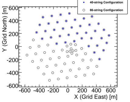
Forty strings of IceCube were in operation from 2008 April 5 to 2009 May 20. The layout of these strings in relation to the final 86-string IceCube configuration is shown in Fig. 1. Over the entire period the detector ran with an uptime of 92%, yielding 375.5 days of total exposure. Deadtime is mainly due to test runs during and after the construction season dedicated to calibrating the additional strings and upgrading data acquisition systems.

X (Grid East) [m]

-600 -400 -200 0 200 400 600

Y (Grid North) [m]

-600 -400 -200 0 200 400 600

40-string Configuration 86-string Configuration

Fig. 1.— Overhead view of the 40-string configuration, along with additional strings that will make up the complete IceCube detector.

IceCube uses a simple multiplicity trigger, requiring local coincidence hits in eight DOMs

within 5 µs. Once the trigger condition is met, local coincidence hits within a readout win-

dow ±10 µs are recorded, and overlapping readout windows are merged together. IceCube

triggers primarily on down-going muons at a rate of about 950 Hz in this (40-string) config-

uration. Variations in the trigger rate by about ±10% are due to seasonal changes affecting development of CR showers and muon production in the atmosphere, with higher rates during the austral summer (Tilav et al. 2010).

3. Data and Simulation 3.1. Data Sample

Traditional astrophysical neutrino point source searches have used the Earth to block all upward traveling (up-going) particles except muons induced by neutrinos, as in Abbasi et al.

(2009b). There remains a background of up-going muons from neutrinos, which are created in CR air showers and can penetrate the entire Earth. These atmospheric neutrinos have a softer energy spectrum than many expectations for astrophysical neutrinos. The measurement of the atmospheric neutrino spectrum for the 40-string detector is discussed in Abbasi et al.

(2010b). A large number of muons produced in CR showers in the atmosphere and moving downward through the detector (down-going) are initially mis-reconstructed as up-going.

These mask the neutrino events until quality selections are made, leaving only a small residual of mis-reconstructed events.

The down-going region is dominated by atmospheric muons that also have a softer spectrum compared to muons induced by astrophysical neutrinos. At present, this large background reduces the IceCube sensitivity to neutrino sources in the southern sky in the sub-PeV energy region. While veto techniques are in development which will enable larger detector configurations to isolate neutrino-induced events starting within the detector, point source searches can meanwhile be extended to the down-going region if the softer-spectrum atmospheric muon background is reduced by an energy selection. This was done for the first time using the previous 22-string configuration of IceCube (Abbasi et al. 2009a), extending IceCube’s field of view to −50 ^◦ declination. In this paper we extend the field of view to −85 ^◦ declination (the exclusion between −85 ^◦ and −90 ^◦ is due to the use of scrambled data for background estimation in the analysis, described in Sec. 5). Down-going muons can also be created in showers caused by gamma rays, which point back to their source like neutrinos.

The possibility for IceCube to detect PeV gamma ray sources in the southern sky is discussed in Halzen et al. (2009), which concludes that a realistic source could be detected using muons in the ice only after 10 years of observing. Gamma ray sources will not be considered further here.

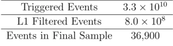
Two processing levels are used to reduce the approximately 3.3 × 10 ¹⁰ triggered events

down to a suitable sample for analysis (see Table 1). Random noise at the level of about

500 Hz per DOM is mainly due to radioactive decays in the materials in the DOMs. The contribution to triggered events by this random noise is highly suppressed by the local coincident hit requirement. To further reduce the contribution from noise, only hits within a 6 µs time window are used for the reconstructions. This time window is defined as the window that contains the most hits during the event. About 5% of down-going muons which trigger the detector are initially mis-reconstructed as up-going by the first stages of event processing. A persistent background that grows with the size of the detector is CR muons (or bundles of muons) from different showers which arrive in coincidence. At trigger level they make up about 13% of the events. These coincident muon bundles can mimic the hit pattern of good up-going events, confusing a single-muon fit.

A likelihood-based muon track reconstruction is first performed at the South Pole (L1 filter). The likelihood function (Ahrens et al. 2004) parameterizes the probability of observ- ing the geometry and timing of the hits in terms of a muon track’s position, zenith angle, and azimuth angle. This likelihood is maximized, yielding the best-fit direction and position for the muon track. Initial fits are performed using a single photoelectron (SPE) likelihood that uses the time of the leading edge of the first photon arriving in each DOM. These re- constructions yield robust results used for the first level of background rejection. All events that are reconstructed as up-going are kept, while events in the down-going region must pass an energy cut that tightens with decreasing zenith angle. Events pass this L1 filter at an average rate of about 22 Hz and are buffered before transmission via a communications satellite using the South Pole Archival and Data Exchange (SPADE) system.

The processing done in the North includes a broader base of reconstructions compared to what is done at the South Pole. Rather than just the simple SPE fit, the multiple photoelectron (MPE) fit uses the number of observed photons to describe the expected arrival time of the first photon. This first photon is scattered less than an average photon when many arrive at the same DOM. The MPE likelihood description uses more available information than SPE and improves the tracking resolution as energy increases, and this reconstruction is used for the final analysis. The offline processing also provides parameters useful for background rejection, reconstructs the muon energy, and estimates the angular resolution on an event-by-event basis. Reducing the filtered events to the final sample of

Table 1. Number of events at each processing level for the 375.5 d of livetime.

Triggered Events 3.3 × 10 ¹⁰

L1 Filtered Events 8.0 × 10 ⁸

Events in Final Sample 36,900

this analysis requires cutting on the following parameters:

• Reduced log-likelihood: The log-likelihood from the muon track fit divided by the number of degrees of freedom, given by the number of DOMs with hits minus five, the number of free parameters used to describe the muon. This parameter performed poorly on low energy signal events. It was found that low energy efficiency could be increased by instead dividing the likelihood by number of DOMs with photon hits minus 2.5. Both the standard and modified parameters were used, requiring events to pass one selection or the other. This kept the efficiency higher for a broader energy range.

• Angular uncertainty, σ: An estimate of the uncertainty in the muon track direction.

The directional likelihood space around the best track solution is sampled and fit to a paraboloid. The contour of the paraboloid traces an error ellipse indicating how well the muon direction is localized (Neunhoffer 2006). The RMS of the major and minor axes of the error ellipse is used to define a circular error. This parameter is effective both for removing mis-reconstructed events and as an event-by-event angular uncertainty estimator.

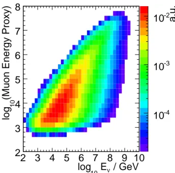
• Muon energy proxy: The average photon density along the muon track, used as a proxy for the muon energy. It is calculated accounting for the distance to DOMs, their angular acceptance, and average scattering and absorption properties of photons in the ice. The energy loss of a muon moving through the detector scales with the muon energy above about 1 TeV when stochastic energy losses due to bremsstrahlung, pair production, and photonuclear interactions dominate with respect to ionization losses. The energy resolution obtained is of the order of 0.3 in the log ₁₀ of the muon energy (at closest approach to the average hit location) for energies between about 10 TeV and 100 PeV. The energy of the parent neutrino can be inferred from the reconstructed muon energy loss in the detector using simulation. Since the interaction vertex is often an unknown distance from the detector, the muon in the detection volume has already lost an unknown amount of energy. Fig. 2 shows the distribution of this energy parameter versus the true neutrino energy for an E ⁻² spectrum. Despite the uncertainty on the neutrino energy, for a statistical sample of events this energy estimator is a powerful analysis tool because of the wide range over which energies are measured.

• Zenith-weighted likelihood ratio: The likelihood ratio between an unbiased muon

fit and a fit with an event weight according to the known down-going muon zenith dis-

tribution as a Bayesian prior. Applied to up-going tracks, a high likelihood ratio estab-

lishes strong evidence that the event is actually up-going and not a mis-reconstructed down-going event.

• NDir: The number of DOMs with direct photons, defined as arriving within -15 ns to +75 ns of the expectation from an unscattered photon emitted from the recon- structed muon track at the Cherenkov angle. Scattering of photons in the ice causes a loss of directional information and will delay them with respect to the unscattered expectation.

• LDir: The maximum length between direct photons, projected along the best muon track solution.

• Zenith directions of split events: The zenith angles resulting from splitting of an event into two parts and reconstructing each part separately. This is done in 2 ways:

temporally, by using the mean photon arrival time as the split criterion; and geomet- rically, by using the plane both perpendicular to the track and containing the average hit location as the split criterion. This technique is effective against coincident muon bundles mis-reconstructed as single up-going tracks if both sub-events are required to be up-going.

/ GeV E ν

log 10

2 3 4 5 6 7 8 9 10 (Muon Energy Proxy) 10 log

2 3 4 5 6 7 8

a.u.

10 -4

10 -3

10 -2

Fig. 2.— Distribution of the muon energy proxy (energy loss observed in the detector) versus

the true neutrino energy for an arbitrary normalization E ⁻² flux.

In the up-going region, all parameters are used. The zenith-weighted likelihood ratio and event splitting are specifically designed to remove down-going atmospheric muon back- grounds that have been mis-reconstructed as up-going while the other parameters focus on overall track quality.

In the down-going region, without a veto or earth filter, muons from CR showers over- whelm neutrino-induced muons, except possibly at high energies if the neutrino source spec- tra are harder than the CR spectrum. The aim of the analysis in this region is therefore to select high energy, well-reconstructed events. We use the first three parameters in the list above as cut variables, requiring a higher track quality than in the up-going range. Energy cuts were introduced in the down-going region to reduce the number of events to a suitable size, cutting to achieve a constant number of events per solid angle (which also simplifies the background estimation in the analysis). This technique keeps the high energy events which are most important for discovery. Cuts were optimized for the best sensitivity using a simulated signal of muon neutrinos with E ⁻² spectrum. We checked that the same cuts resulted in a nearly optimal sensitivity for a softer E ⁻³ spectrum in the up-going region where low energy sensitivity is possible and for a harder E ^−1.5 spectra in the down-going region.

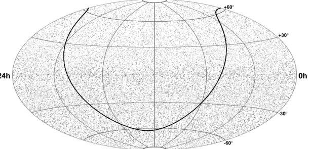
Of the 36,900 events passing all selection criteria, 14,121 are up-going events from the northern sky, mostly muons induced by atmospheric neutrinos. Simulations of CR air show- ers with CORSIKA show a 2.4±0.8% contamination due to mis-reconstructed down-going atmospheric muons. The other 22,779 are down-going events from the southern sky, mostly high energy atmospheric muons. An equatorial sky map of these events is given in Fig. 3.

3.2. Data and Simulation Comparison

Simulation of neutrinos is used for determining event selection and calculating upper limits. The simulation of neutrinos is based on ANIS (Gazizov & Kowalski 2005). Deep in- elastic neutrino-nucleon cross sections use CTEQ5 parton distribution functions (Lai et al.

2000). Neutrino simulation can be weighted for different fluxes, accounting for the probability of each event to occur. In this way, the same simulation sample can be used to represent at- mospheric neutrino models such as Bartol (Barr et al. 2004) and Honda (Honda et al. 2007) neutrino fluxes from pion and kaon decays (conventional flux). Neutrinos from charmed me- son decays (prompt flux) have been simulated according to a variety of models (Martin et al.

2003; Enberg et al. 2008; Bugaev 1989). Seasonal variations in atmospheric neutrino rates are expected to be a maximum of ±4% for neutrinos originating near the polar regions.

Near the equator, atmospheric variations are much smaller and the variation in the number

24h 0h

° +30

° +60

° -30

° -60

Fig. 3.— Equatorial skymap (J2000) of the 36,900 events in the final sample. The galactic plane is shown as the solid black curve. The northern sky (positive declinations) is dominated by up-going atmospheric neutrino-induced muons, and the southern sky (negative declina- tions) is dominated by muons produced in cosmic ray showers in the atmosphere above the South Pole.

of events is expected to be less than ±0.5% (Ackermann & Bernardini 2005).

Atmospheric muon background is simulated mostly to guide and verify the event selec- tion. Muons from CR air showers were simulated with CORSIKA (Heck et al. 1998) with the SIBYLL hadronic interaction model (Ahn et al. 2009). An October polar atmosphere, an average case over the year, is used for the CORSIKA simulation, ignoring the seasonal variations of ±10% in event rates (Tilav et al. 2010). Muon propagation through the Earth and ice are done using MMC (Chirkin & Rhode 2004). Using measurements of the scattering and absorption lengths in ice (Ackermann et al. 2006), a detailed simulation propagates the photon signal to each DOM (Lundberg et al. 2007). The simulation of the DOMs includes their angular acceptance and electronics. Experimental and simulated data are processed and filtered in the same way.

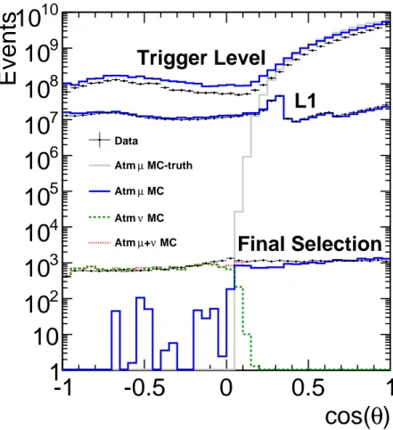
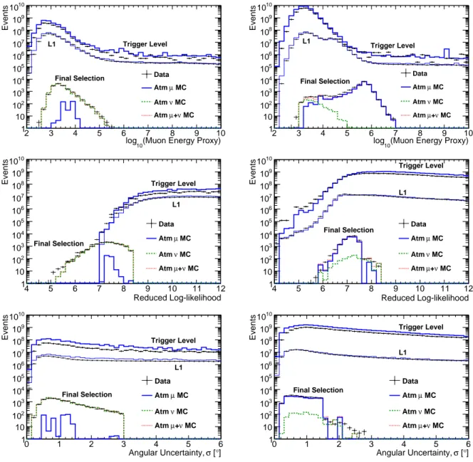
In Fig. 4 we show the cosine of zenith and in Fig. 5 the muon energy proxy, reduced

log-likelihood, and angular uncertainty estimator distributions of all events at trigger level,

L1 filter level, and after final analysis cuts for data and Monte Carlo (MC). In these figures,

the simulation uses a slightly modified version of the poly-gonato model of the galactic CR

flux and composition (Hoerandel 2003). Above the galactic model cutoff at Z × 4 × 10 ¹⁵ eV,

a flux of pure iron is used with an E ⁻³ spectrum. This is done because currently CORSIKA cannot propagate elements in the poly-gonato model that are heavier than iron. Moreover, the poly-gonato model only accounts for galactic CRs and does not fully account for the average measured flux above 10 ¹⁷ eV, even when all nuclei are considered (see Fig. 11 in Hoerandel (2003)). These corrections then reproduce the measured CR spectrum at these energies. There is a 23% difference in normalization of data and CR muon events at trigger level. This normalization offset largely disappears after quality cuts are made. Generally good agreement is achieved at later cut levels. Some remaining disagreements are discussed further in Sec. 7, along with the impact of using different CR primary models.

4. Detector Performance

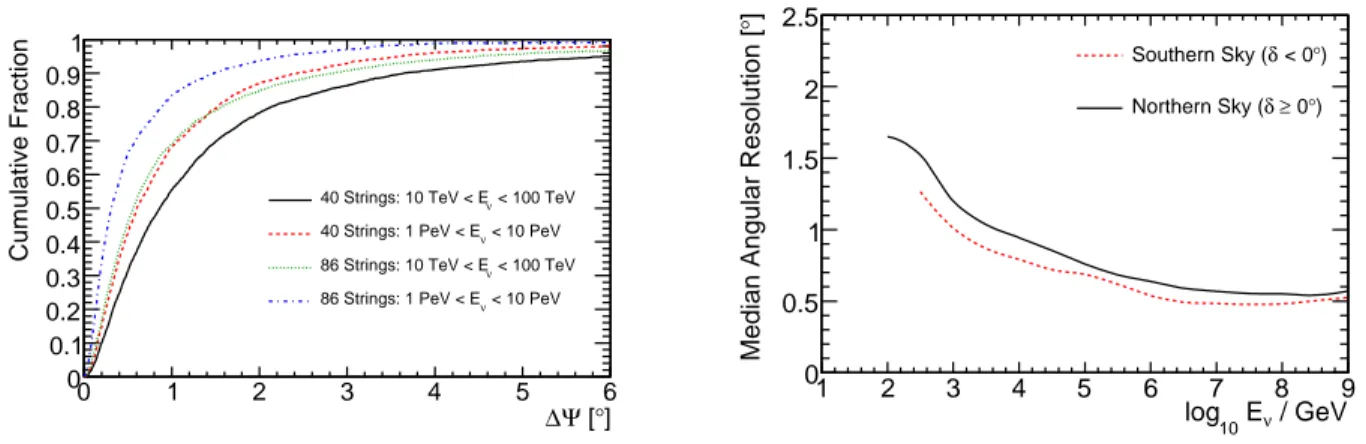
The performance of the detector and the analysis is characterized using the simulation described in Sec. 3.2. For an E ⁻² spectrum of neutrinos, the median angular difference between the neutrino and the reconstructed direction of the muon in the northern (southern) sky is 0.8 ^◦ (0.6 ^◦ ). Along with more severe quality selection in the southern sky, the different energy distributions in each hemisphere, shown in Fig. 6, cause the difference in these two values. This is because the reconstruction performs better at higher energy due to the larger amount of light and longer muon tracks. The cumulative point spread function (PSF) is shown in Fig. 7 for two energy ranges and compared with simulation of the complete IceCube detector using the same quality selection, as well as the median PSF versus energy for the two hemispheres.

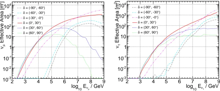
The neutrino effective area A ^eff _ν is a useful parameter to determine event rates and the performance of a detector for different analyses and fluxes. The expected event rate for a given differential flux dN/dE is

N events = Z

dE ν A ^eff _ν (E ν , δ ν ) dN ν (E ν , δ ν ) dE ν

, (1)

and is calculable using simulation. The A ^eff _ν represents the size of an equivalent detector if it were 100% efficient. Figure 8 shows the A ^eff _ν for fluxes of ν _µ + ¯ ν _µ and ν _τ + ¯ ν _τ , for events at final selection level. Neutrinos arriving from the highest declinations must travel through the largest column depth and can be absorbed: this accounts for the turnover at high energies for nearly vertical up-going muon neutrinos. Tau neutrinos have the advantage that the tau secondary can decay back into a tau neutrino before losing much energy.

Although tau (and electron) neutrino secondaries usually produce nearly-spherical show-

ers rather than tracks, tau leptons will decay to muons with a 17.7% branching ratio

θ ) cos(

-1 -0.5 0 0.5 1

Events

1 10 10 2

10 3

10 4

10 5

10 6

10 7

10 8

10 9

10 10

Trigger Level

L1

Final Selection

Data

MC-truth µ

Atm µ MC Atm

ν MC Atm

ν MC µ + Atm

Fig. 4.— Distribution of reconstructed cosine zenith at trigger level, L1, and final cut level for data and simulation of atmospheric muons (Hoerandel 2003) and neutrinos (Barr et al.

2004; Bugaev 1989). The true cosine zenith distribution of the muons at trigger level is also shown. For the final sample, the deficit of simulation seen near the horizon is discussed in Sec. 7, along with comparisons to other models. The deficit is most likely caused by a deficiency in knowledge of the CR composition in the region around the knee. More detailed comparisons are discussed in Sec 7, including comparisons to a variety of models.

(Amsler et al. 2008). At very high energy (above about 1 PeV) a tau will travel far enough

before decaying that the direction can be reconstructed well, contributing to any extrater-

restrial signal in the muon channel. For the upper limits quoted in Sec. 8, we must make

an assumption on the flavor ratios at Earth, after oscillations. It is common to assume

Φ _ν

: Φ _ν

: Φ _ν

= 1 : 1 : 1. This is physically motivated by neutrino production from pion

decay and the subsequent muon decay, yielding Φ _ν

: Φ _ν

: Φ _ν

= 1 : 2 : 0. After stan-

(Muon Energy Proxy) log

2 3 4 5 6 7 8 9 10

Events

1 10 10

10

10

10

10

10

10

10

10

Trigger Level L1

Final Selection Data

µ MC Atm

ν MC Atm

ν MC µ+ Atm

(Muon Energy Proxy) log

2 3 4 5 6 7 8 9 10

Events

1 10 10

10

10

10

10

10

10

10

10

Trigger Level L1

Final Selection

Data µ MC Atm

ν MC Atm

ν MC µ+ Atm

Reduced Log-likelihood

4 5 6 7 8 9 10 11 12

Events

1 10 10

10

10

10

10

10

10

10

10

Trigger Level L1

Final Selection

Data µ MC Atm

ν MC Atm

ν MC µ+ Atm

Reduced Log-likelihood

4 5 6 7 8 9 10 11 12

Events

1 10 10

10

10

10

10

10

10

10

10

L1

Final Selection Data µ MC Atm

ν MC Atm

ν MC µ+ Atm

° ] σ [ Angular Uncertainty,

0 1 2 3 4 5 6

Events

1 10 10

10

10

10

10

10

10

10

10

Trigger Level

L1

Final Selection

Data µ MC Atm

ν MC Atm

ν MC µ + Atm

° ] σ [ Angular Uncertainty,

0 1 2 3 4 5 6

Events

1 10 10

10

10

10

10

10

10

10

10

Trigger Level

L1

Final Selection

Data µ MC Atm

ν MC Atm

ν MC µ + Atm

Fig. 5.— Distributions of muon energy proxy (top row), reduced log-likelihood (middle row), and angular uncertainty estimator (bottom row) for the up-going sample (left column) and the down-going sample (right column). Each is shown at trigger level, L1, and final cut level for data and simulation of atmospheric muons and neutrinos. In the up-going sample (left column), all atmospheric muons are mis-reconstructed, and at final level their remaining estimated contribution is about 2.4±0.8%.

dard oscillations over astrophysical baselines, this gives an equal flux of each flavor at Earth

(Athar et al. 2000). Under certain astrophysical scenarios, the contribution from muon de-

cay may be suppressed, leading to an observed flux ratio of Φ _ν

: Φ _ν

: Φ _ν

= 1 : 1.8 : 1.8

/ GeV E ν

log 10

2 3 4 5 6 7 8 9 10

) δ sin(

-1 -0.8 -0.6 -0.4 -0.2 0 0.2 0.4 0.6 0.8 1

a.u.

10 -5

10 -4

10 -3

Fig. 6.— Energy distribution for an arbitrary normalization E ⁻² flux of neutrinos as a function of declination for the final event selection. The black contours indicate the 90%

central containment interval for each declination.

° ] Ψ [

0 1 2 3 4 5 ∆ 6

Cumulative Fraction

0 0.1 0.2 0.3 0.4 0.5 0.6 0.7 0.8 0.9 1

< 100 TeV 40 Strings: 10 TeV < Eν

< 10 PeV 40 Strings: 1 PeV < Eν

< 100 TeV 86 Strings: 10 TeV < Eν

< 10 PeV 86 Strings: 1 PeV < Eν

/ GeV E

log

1 2 3 4 5 6 7 8 9

] ° Median Angular Resolution [

0 0.5 1 1.5 2 2.5

° ) < 0 δ Southern Sky (

° )

≥ 0 δ Northern Sky (

Fig. 7.— Cumulative point spread function (angle between neutrino and reconstructed muon

track) for simulated E ⁻² neutrino signal events at the final cut level in the up-going region

(left). Also shown is the final IceCube configuration. The median of the PSF versus energy

is shown separately for the northern and southern skies (right). The improvement in the

southern sky is because of the more restrictive quality cuts.

(Kashti & Waxman 2005), or the contribution of tau neutrinos could be enhanced by the decay of charmed mesons at very high energy (Enberg et al. 2009). For an E ⁻² spectrum and equal muon and tau neutrino fluxes, the fraction of tau neutrino-induced events is about 17% for vertically down-going, 10% near the horizon, and 13% for vertically up-going. Be- cause the contribution from tau neutrinos is relatively small, assuming only a flux of muon neutrinos can be used for convenience and to compare to other published limits. We have tabulated limits on both Φ ν

and the sum Φ ν

+ Φ ν

, assuming an equal flux of each, while in the figures we have specified that we only consider a flux of muon neutrinos. Limits are always reported for the flux at the surface of the Earth.

/ GeV

ν

10 E log

2 3 4 5 6 7 8 9

] 2 Effective Area [m µ ν

10 -3

10 -2

10 -1

1 10 10 2

10 3

10 4 _{δ = (-90 ° , -60 ° )}

° ) , -30

° = (-60 δ

° )

° , -0 = (-30 δ

° )

° , 30 = (0 δ

° )

° , 60 = (30 δ

° )

° , 90 = (60 δ

/ GeV

ν

10 E log

2 3 4 5 6 7 8 9

] 2 Effective Area [m τ ν

10 -3

10 -2

10 -1

1 10 10 2

10 3

10 4 _{δ = (-90 ° , -60 ° )}

° ) , -30

° = (-60 δ

° )

° , -0 = (-30 δ

° )

° , 30 = (0 δ

° )

° , 60 = (30 δ

° )

° , 90 = (60 δ

Fig. 8.— Solid-angle-averaged effective areas at final cut level for astrophysical neutrino fluxes in six declination bands for ν µ + ¯ ν µ (left) and ν τ + ¯ ν τ (right), assuming an equal flux of neutrinos and anti-neutrinos.

5. Search Method

An unbinned maximum likelihood ratio method is used to look for a localized, statisti- cally significant excess of events above the background. We also use energy information to help separate possible signal from the known backgrounds.

The method follows that of Braun et al. (2008). The data is modeled as a two component mixture of signal and background. A maximum likelihood fit to the data is used to determine the relative contribution of each component. Given N events in the data set, the probability density of the i ^th event is

n s

N S i + (1 − n s

N )B i , (2)

where S i and B i are the signal and background probability density functions (PDFs), re- spectively. The parameter n s is the unknown contribution of signal events.

For an event with reconstructed direction ~x i = (α i , δ i ), we model the probability of originating from the source at ~x s as a circular 2-dimensional Gaussian,

N (~x _i ) = 1 2πσ ² _i e ⁻

|~xi−~xs|2 2σ2

i

, (3)

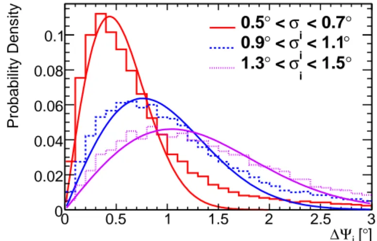
where σ i is the angular uncertainty reconstructed for each event individually (Neunhoffer 2006) and |~x i − ~x s | is the space angle difference between the source and reconstructed event.

The PSF for different ranges of σ i are in Fig. 9, showing the correlation between the estimated angular uncertainty and track reconstruction error.

° ]

i [ Ψ

0 0.5 1 1.5 2 2.5 ∆ 3

Probability Density

0 0.02 0.04 0.06 0.08

0.1 < 0.7 °

σ i

<

°

0.5 < 1.1 ° σ i

<

° 0.9

° < 1.5 σ i

<

° 1.3

Fig. 9.— Angular deviation between neutrino and reconstructed muon direction ∆Ψ for ranges in σ i , the reconstructed angular uncertainty estimator. Fits of these distributions to 2-dimensional Gaussians projected into ∆Ψ are also shown. The value of σ _i is correlated to the track reconstruction error. A small fraction of events are not well-represented by the Gaussian distribution, but these are the least well-reconstructed events and contribute the least to signal detection.

The energy PDF E (E i |γ, δ _i ) describes the probability of obtaining a reconstructed muon

energy E _i for an event produced by a source of a given neutrino energy spectrum E ^−γ at dec-

lination δ _i . We describe the energy distribution using 22 declination bands. Twenty bands,

spaced evenly by solid angle, cover the down-going range where the energy distributions are

changing the most due to the energy cuts in the event selection, while two are needed to

sufficiently describe the up-going events, with the separation at δ = 15 ^◦ . We fit the source

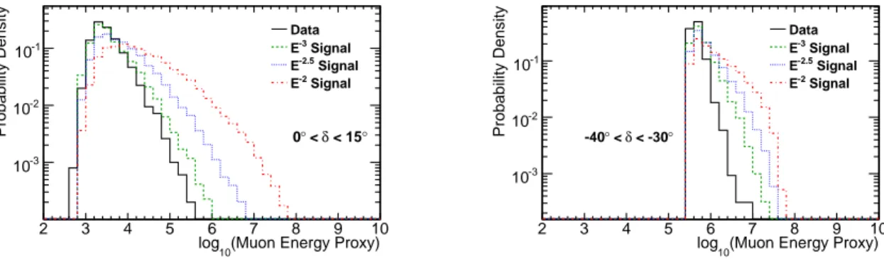
spectrum with a power law E ^−γ ; γ is a free parameter. The probability of obtaining a re- constructed muon energy E i for an event produced by a source with spectral index γ, for spectral indices 1.0 < γ < 4.0, is determined using simulation. Two examples of these energy PDFs are shown in Fig. 10.

(Muon Energy Proxy) log

2 3 4 5 6 7 8 9 10

Probability Density

10

10

10

Data Signal E-3

Signal E-2.5

Signal E-2

° < 15 δ <

° 0

(Muon Energy Proxy) log

2 3 4 5 6 7 8 9 10

Probability Density

10

10

10

Data Signal E-3

Signal E-2.5

Signal E-2

° < -30 δ <

° -40

Fig. 10.— Probability densities for the muon energy proxy for data as well as simulated power-law neutrino spectra. Two declination bands are shown: 0 ^◦ < δ < 15 ^◦ (left) and

−40 ^◦ < δ < −30 ^◦ (right), representing two of the declination-dependent energy PDFs used in the likelihood analysis. There is an energy cut applied for negative declinations.

The full signal PDF is given by the product of the spatial and energy PDFs:

S _i = N (~x i ) · E (E i |γ, δ _i ). (4) The background PDF B _i contains the same terms, describing the angular and energy distributions of background events:

B _i = N _Atm (~x i ) · E (E i |Atm, δ _i ), (5)

where N Atm (~x i ) is the spatial PDF of atmospheric background and E (E i |Atm, δ i ) is the

probability of obtaining E i from atmospheric backgrounds (neutrinos and muons) at the

declination of the event. These PDFs are constructed using data and, for the energy term,

in the same 22 declinations bands as the signal PDF. All non-uniformities in atmospheric

background event rates caused by the detector acceptance or seasonal variation average out

in the time-integrated analysis. Therefore N _Atm (~x _i ) has a flat expectation in right ascension

and is only dependent on declination. Because the data are used in this way for background

estimation, the analysis is restricted from −85 ^◦ to 85 ^◦ declination, so that any point source

signal will still be a small contribution to the total number of events in the same declination

region.

The likelihood of the data is the product of all event probability densities:

L(n s , γ) =

N

Y

i=1

h n s

N S i + (1 − n s

N )B i

i . (6)

The likelihood is then maximized with respect to n s and γ, giving the best fit values ˆ n s and ˆ

γ. The null hypothesis is given by n s = 0 (γ has no meaning when no signal is present). The likelihood ratio test statistic is

T S = −2 log h L(n s = 0) L(ˆ n s , γ ˆ s )

i

. (7)

The significance of the analysis is determined by comparing the T S from the real data with the distribution of T S from the null hypothesis (events scrambled in r.a.). We define the p-value as the fraction of randomized data sets with higher test statistic values than the real data. We evaluate the median sensitivity and upper limits at a 90% confidence level (CL) using the method of Feldman & Cousins (1998) and calculate the discovery potential as the flux required for 50% of trials with simulated signal to yield a p-value less than 2.87 × 10 ⁻⁷ (i.e. 5σ significance if expressed as the one-sided tail of a Gaussian distribution).

The distribution of T S for 10 million trials is shown in Fig. 11 for a fixed point source at δ = 45 ^◦ . Distributions with simulated E ⁻² signal events injected are included, as well as a χ ² distribution with 2 degrees of freedom, which is used to estimate the 5σ significance threshold for calculating the discovery potential since simulating enough scrambled data sets requires a large amount of processing time.

Although E ⁻² sensitivities and limits have become a useful benchmark for comparing performance, a wide range of other spectral indices are possible along with cutoffs over a wide range of energy. To understand the ability of the method to detect sources with cut-off spectra, typically observed in gamma rays to be in the range 1–10 TeV for galactic sources, Fig. 12 shows the discovery potentials for a wide range of exponential cut-offs, demonstrating the ability of the method to detect sources with cut-off spectra. Typically, cut-offs observed in gamma rays are in the range 1–10 TeV for galactic sources. The likelihood fit is still performed using a pure power law.

The likelihood analysis is not only more sensitive than binned methods, but it can also

help extract astrophysical information. Fig. 13 shows our ability to reconstruct the spectral

index for power law neutrino sources at a declination of 6 ^◦ . The effective area is high for a

broad range of energies here, and the spectral resolution is best. For each spectrum shown,

the statistical uncertainty (1σ CL) in the spectral index will be about ±0.3 when enough

events are present to claim a discovery. Spectral resolution worsens for sources farther from

TS 0 5 10 15 20 25 30 35 40 45

Trials

1 10 10 2

10 3

10 4

10 5

10 6

10 7

10 8 ^{BG only}

approximation χ

BG + 4 Signal Events BG + 8 Signal Events BG + 12 Signal Events

Fig. 11.— Distribution of the test statistic T S for a fixed point source at δ = 45 ^◦ . Statistical errors are shown for the background-only distribution using 10 million scrambled data sets.

A χ ² distribution with 2 degrees of freedom can be used as an approximation. Also shown are the distributions when simulated E ⁻² signal events are injected. About 12 events on average are needed for a discovery at this declination.

the horizon, to ±0.4 at both δ = −45 ^◦ and δ = 45 ^◦ when enough events are present for a discovery in each case.

Stacking multiple sources in neutrino astronomy has been an effective way to enhance discovery potential and further constrain astrophysical models (Achterberg et al. 2006b;

Abbasi et al. 2009c). We can consider the accumulated signal from a collection of sources using a method similar to Abbasi et al. (2006). Only a modification to the signal likelihood is necessary in order to stack sources, breaking the signal hypothesis into the sum over M sources:

S _i ⇒ S _i ^tot = P M

j=1 W ^j R ^j (γ)S _i ^j P M

j=1 W ^j R ^j (γ ) , (8)

where W ^j is the relative theoretical weight, R ^j (γ) is the relative detector acceptance for a

source with spectral index γ (assumed to be the same for all stacked sources), and S _i ^j is the

signal probability density for the i ^th event, all for the j ^th source. As before, the total signal

events n _s and collective spectral index γ are fit parameters. The W ^j coefficients depend on

/ GeV

cutoff 10

E

2 3 4 5 6 log 7 8 9

]

s

cm

[TeV

Φ

10

10

10

10

10

δ = -45 °

° δ = 0

° = 45 δ

/ GeV

cutoff 10

E

2 3 4 5 6 log 7 8 9

Events

0 5 10 15 20 25 30

° = -45 δ = 0 ° δ = 45 ° δ

Fig. 12.— Flux normalization (left) and number of events at the final level (right) for discovery potential versus an exponential cutoff for a differential flux parametrized as dN/dE = Φ ⁰ · (E/TeV) ⁻² exp(−E/E _cutoff ). Curves are shown at three representative de- clinations. The likelihood fit is still performed using a pure power law.

Number of Signal Events 0 2 4 6 8 10 12 14 16 18 20 22 24

Spectral Index

1 1.5 2 2.5 3 3.5 4

Fig. 13.— Reconstructed spectral index (1σ shaded area) versus the number of signal events

injected for three source spectra: E ^−1.5 , E ⁻² , and E ⁻³ . The sources are pure power-laws at

a declination of 6 ^◦ . The stars mark the number of events required for a 5σ discovery for each

spectrum. Systematic errors are not included.

our prior theoretical assumptions about the expected neutrino luminosity. They are higher for sources that are, on theoretical grounds, expected to be brighter. Tables for R ^j (γ), given as the mean number of events from a source with dN/dE ∝ E ^−γ , are calculated using simulation. The flexibility built into the method by the relative detector acceptance and theoretical weights allows us to use source catalogs covering the whole sky and with large variations in source strengths, as well as to directly test model predictions. The improvement in discovery potential from stacking sources is illustrated in Fig. 14, showing the discovery potential flux versus the number of sources stacked. All sources are at the same declination in this example.

Number of Sources Stacked

0 10 20 30 40 50

] -1 s -2 TeV cm -11 dN/dE [10 2 E

10 -1

1 10

Total Flux for Discovery

Flux per Source for Discovery

Fig. 14.— Discovery potential flux versus the number of stacked sources, all with an equal E ⁻² flux and (for example purposes) at a fixed declination of 45 ^◦ . Although the total flux required increases as more sources are added, owing to a higher effective background, the flux per source required can be substantially reduced.

We would also like to consider sources that are spatially extended (with respect to

the point spread function). For an example of how important this can be, the significance

observed by the Milagro experiment in the location of the Fermi source J0634.0+1745 (as-

sociated with the Geminga pulsar) rises from 3.5σ to 6.3σ by fitting for an extended source

(Abdo et al. 2009). The only modification to the method required is to convolve the source

distribution with the point spread function. Since we model our point spread function as a

circular 2-dimensional Gaussian distribution, it is easy to also model a source as a circular

2-dimensional Gaussian of width σ s . The convolution results in a broader 2-dimensional Gaussian of width p

σ ² _i + σ _s ² and the likelihood uses this distribution for the signal spatial term. The discovery potential flux for a range of source extensions is shown in Fig. 15 and compared to the (incorrect) hypothesis of a point source. For a source with true ex- tent σ _s = 2 ^◦ , the point-source hypothesis requires nearly a factor of 2 times more flux for discovery compared to the correct extended-source hypothesis.

° ]

s [

0 1 2 3 4 5 6 7 σ 8

] -1 s -2 TeV cm -11 dN/dE [10 2 E

0 5 10 15 20 25 30 35

Point-Source Hypothesis

Extended-Source Hypothesis

Fig. 15.— Discovery potential flux versus the σ s of an extended source (distributed as a 2-dimensional Gaussian) with an E ⁻² spectrum at a declination of 25 ^◦ . The case of a point- source hypothesis is compared against the correct extended-source hypothesis matching what was used to simulate the signal.

6. Description of the Five Searches We have performed five searches:

1. a scan for the most significant point source in the entire sky;

2. a search over an a priori defined list of 39 interesting astrophysical objects;

3. a stacking search for 16 Milagro TeV gamma ray sources, some seen only in coincidence

with the Fermi-LAT, and one unconfirmed hot spot (17 total sources);

4. a stacking search for 127 local starburst galaxies (Becker et al. 2009);

5. a stacking search for five nearby clusters of galaxies (CGs), testing four different models for the CR spatial distribution (Murase et al. 2008).

The analyses and event selection procedure were determined before unblinding the r.a.

of the data. We require a 5σ significance for discovery. Final p-values are calculated for each search individually.

6.1. All-sky Scan

The first search is a scan for the single most significant point source of neutrinos over the declination range −85 ^◦ to +85 ^◦ . The maximum likelihood ratio is defined continuously over the sky, and we sample it on a grid of 0.1 ^◦ in r.a. and 0.1 ^◦ in dec. The size of the grid is not important as long as it is small compared to the angular resolution of the detector.

Using a finer grid increases the computation time with no added benefit. A grid size that is comparable to or larger than the angular resolution could miss the location of the peaks in the significance map, yielding sub-optimal performance.

6.2. A Priori Source List

In order to avoid the large number of effective trials associated with scanning the entire sky, we also perform a search for the most significant of 39 a priori selected source candidates, given in Table 3. These sources have been selected on the basis of observations in gamma rays or astrophysical modeling that predicts neutrino emission. We also added the most significant location observed in the 22-string IceCube configuration (a post-trial p-value of 1.3% (Abbasi et al. 2009b)).

6.3. Milagro TeV Source Stacking

The Milagro Collaboration has reported 16 sources of TeV gamma rays (Abdo et al.

2007), several only after correlating with GeV gamma rays from the Fermi Gamma-ray Space Telescope source list (Abdo et al. 2009). These sources are promising candidates for detection by neutrino telescopes. Particularly interesting are sources in the complex Cygnus region (Beacom & Kistler 2007) and six supernova remnant associations (Halzen et al. 2008;

Gonzalez-Garcia et al. 2009), including MGRO J1852+01, a hot spot that falls below the

significance threshold of the Milagro Coll. to be claimed as a source. If confirmed as a source, MGRO J1852+01 could contribute a large fraction (about 42%) of the total neutrino flux from the SNR sources (Halzen et al. 2008). For the 40-string configuration of IceCube, the model of Halzen et al. (2008) predicts 3.0 neutrino events in 375.5 days, following an E ^−2.1 spectrum with an exponential cutoff at about 600 TeV.

We performed a stacking search for 17 sources observed in TeV gamma rays by Milagro (adding MGRO J1852+01 to the 16 sources which were found significant by the Milagro Coll.) using an equal weight for each source in the likelihood. Assuming that neutrino and gamma ray fluxes correlate and using these as weights in the likelihood did not appreciably improve the sensitivity in this case. Spatial extensions were used in the search for three of the sources where measurements were given (also used in the source simulation for limit calculations). The largest source was MGRO J2031+41, reported to have a diameter of 3.0 ^◦ ± 0.9 ^◦ .

6.4. Starburst Galaxy Stacking

Starburst galaxies have a dense interstellar medium and high star formation rates, par- ticularly of high-mass stars. This leads to both high supernova rates and heating of ambient dust. The model of Becker et al. (2009) associates the far infrared (FIR) emission with this hot dust and the radio emission with synchrotron losses of CR electrons, presumably ac- celerated along with hadronic CRs in the elevated number of SNRs. The observed strong correlation between the FIR and radio emission points to the high star formation rate as the single underlying cause, and should also correlate with the neutrino flux. The increased production of CRs and high density of target material are ideal conditions for neutrino pro- duction. The starburst galaxies M82 and NGC 253 have been observed in gamma rays at GeV–TeV energies (Abdo et al. 2010; Acciari et al. 2009; Aharonian et al. 2005) and are the only observed steady extragalactic TeV gamma ray sources not associated with AGNs.

We performed a stacking search for 127 starburst galaxies, weighting the sources by their observed FIR flux at 60 µm, as compiled in Table A.1 in Becker et al. (2009).

6.5. Galaxy Cluster Stacking

Clusters of galaxies (CGs) are another potential source of high energy protons and,

through interactions with intracluster material (ICM), neutrinos. CGs are the largest gravi-

tationally bound objects in the Universe and continue to grow through merging and accretion

of dark matter and baryonic gas, generating shock fronts on megaparsec scales. The possi- bility for CGs to be sources of ultra high energy CRs above 3 × 10 ¹⁸ eV is described in, e.g., Norman et al. (1995); Kang et al. (1997). Murase et al. (2008) discuss the possibility of CGs being a significant contribution to the CR spectrum between the second knee at about 3×10 ¹⁷ eV and the ankle at about 3 × 10 ¹⁸ eV. They give predictions for neutrinos from five nearby (z < 0.03) CGs: Virgo, Centaurus, Perseus, Coma, and Ophiuchus. Information on location, distance, and size of CGs (virial radii) was taken from Reiprich & Boehringer (2002). These nearby CGs appear to us as spatially extended objects with virial radii subtending 1.3 ^◦ –6.9 ^◦ , so an extended spatial distribution of neutrinos is possible. Whereas the distribution of the ICM is well known from X-ray observations (Pfrommer & Ensslin 2004), the distribution of CRs is highly uncertain. The distribution of neutrinos is given by the product of the CR and ICM distributions. Four CR models have been considered for neutrino production, discussed in Murase et al. (2008) and references therein (e.g., (Colafrancesco & Blasi 1998;

Berezinsky et al. 1997)):

• Model A: CRs are uniformly distributed within the cluster shock radius, taken to be 0.56 of the virial radius for the dynamical parameters considered.

• Model B: CRs are uniformly distributed within the virial radius, yielding the most conservative neutrino flux distributed over the largest area.

• Isobaric: CRs follow the distribution of thermal gas.

• Central AGN: In a two-step acceleration scenario CRs are accelerated in the central AGN up to a maximum energy before diffusing throughout the cluster and possibly undergoing further acceleration. For the purposes of IceCube searches, this model can be treated as a point source. This model is discussed in detail by Kotera et al. (2009).

Signal neutrinos were simulated according to each of the four models. We modeled the source extensions in the likelihood as 2-dimensional Gaussian distributions with the width for each source and each model determined by optimizing for the best discovery potential.

Although the modeling of the source extension as a Gaussian in the likelihood is not ideal, it is straightforward and computationally fast. The exact shape of the sources is not important for small signals; we may be able to analyze the shape with more detail depending on the intensity of any signal.

We performed a stacking search for five nearby CGs mentioned above following the model

predictions of Murase et al. (2008) as weights in the likelihood. The size of the clusters in

the likelihood fit was allowed to vary discretely between the optimal widths for each CR