Astrophysical Tau Neutrinos in IceCube

(1)

Astrophysical Tau Neutrinos in IceCube

DISSERTATION

zur Erlangung des akademischen Grades doctor rerum naturalium

(Dr. rer. nat.) im Fach Physik eingereicht an der

Mathematisch-Naturwissenschaftlichen Fakult¨at der Humboldt-Universit¨at zu Berlin

von

Juliana Stachurska, M.Sc.

Pr¨asidentin der Humboldt-Universit¨at zu Berlin:

Prof. Dr.-Ing. Dr. Sabine Kunst

Dekan der Mathematisch-Naturwissenschaftlichen Fakult¨at:

Prof. Dr. Elmar Kulke

Gutachter: 1. Prof. Dr. Marek Kowalski, Humboldt-Universit¨at zu Berlin.

2. PD Dr. rer. nat. Walter Winter, Humboldt-Universit¨at zu Berlin.

3. Prof. Dr. Claudio Kopper, Michigan State University, MI, USA.

Tag der m¨undlichen Pr¨ufung: 30. April 2020

(2)

(3)

Abstract

The IceCube neutrino observatory at the South Pole has confirmed the existence of a diffuse astrophysical neutrino flux and measured it in multiple channels. While the first extragalactic neutrino source has likely been identified, the sources of the majority of astrophysical neutrinos remain unknown. The flavor composition of astrophysical neutrinos carries information on the environments at the sites of cosmic particle acceleration as well as potential imprints of new physics acting during neutrino propagation. To tightly constrain the flavor composition the observation of the long-elusive tau neutrinos is required.

Starting at an energy of∼ O(100TeV) a tau neutrino charged current interaction can produce a double cascade topology, where the two energy depositions from the tau creation and the tau decay vertices are resolvable in IceCube. This topology together with the well-established track and single cascade topology is used to measure the flavor composition on Earth. In this work, high-energy events starting in IceCube’s detector volume are classified algorithmically into the three topologies. In the dataset with a livetime of 7.5 years, two events are classified as double cascades for the first time, yielding multi-TeV tau-neutrino candidates. Their observation is consistent with the expectation, assuming astrophysical neutrinos and standard neutrino oscillations. The reconstructed properties of the two tau-neutrino candidates are investigated in more detail in an a-posteriori analysis, making use of targeted Monte-Carlo simulation. The statistical method to constrain the flavor composition is improved by performing a log-likelihood-ratio test using multi-dimensional probability densities. The probability of each of the tau-neutrino candidates to stem from a tau-neutrino interaction versus any other scenario is assessed.

One of the double cascades is consistent with being a misclassified single cascade, while the second double cascade is found to have a misclassification probability of only 3%.

A new flavor composition measurement is performed using the new multi-dimensional likelihood. The measured flavor compositionν_e:ν_µ:ν_τ = 0.20 : 0.39 : 0.42 is consistent with astrophysical neutrinos from all possible astrophysical production mechanisms, as well as with all previously published results. The astrophysical tau-neutrino flux is measured to ^dΦ_dE^ντ

ν = 3.0^+2.2_−1.8·( _E

100 TeV

)−2.87

·10⁻¹⁸·GeV⁻¹cm⁻²s⁻¹sr⁻¹ with spectral index γ = 2.87^+0.21_−0.20, yielding the first non-zero results for the tau normalization. The absence of an astrophysical tau-neutrino flux is disfavored at 2.8σ.

(4)

(5)

Zusammenfassung

Das IceCube Neutrino Observatorium am Südpol hat die Existenz eines diffusen astrophysikalischen Neutrinoflusses nachgewiesen und ihn in mehreren Kanälen mit hoher Signifikanz gemessen. Obwohl die erste wahrscheinliche extragalaktische Neutrinoquelle identifiziert wurde, bleiben die Quellen der Mehrheit der astrophysikalischen Neutri- nos unbekannt. Die Flavor-Zusammensetzung astrophysikalischer Neutrinos trägt In- formationen sowohl über die Orte kosmischer Teilchenbeschleunigung, als auch über die Auswirkungen potenzieller neuer Physik auf die Neutrinoausbreitung. Zur Bestim- mung der Flavor-Zusammensetzung ist die Beobachtung der lange nicht fassbaren Tau- Neutrinos von Nöten. Ab einer Energie von ∼ O(100TeV) kann die Wechselwirkung eines Tau-Neutrinos über geladene Ströme eine Doppelkaskaden-Topologie ergeben, bei der die zwei Energiedepositionen am Tau-Entstehungsvertex und dem Tau-Zerfallsvertex in IceCube aufgelöst werden können. Diese Topologie wird zusammen mit den bereits bekannten Topologien einer Einzel-Kaskade und einer Spur zur Messung der Flavor- Zusammensetzung auf der Erde benutzt. In dieser Arbeit werden im Detektorvolu- men von IceCube anfangende Ereignisse mit hohen Energien algorithmisch in die drei Topologien klassifiziert. Im Datensatz mit einer Lebensdauer von 7.5 Jahren werden zum ersten Mal zwei Ereignisse als Doppelkaskaden klassifiziert; diese sind Kandidaten für multi-TeV Tau-Neutrinos. Deren Beobachtung entspricht den Erwartungen von astrophysikalischen Neutrinos und standard Flavor-Oszillationen. Die rekonstruierten Eigenschaften der zwei Tau-Neutrino-Kandidaten werden mithilfe gezielter Monte-Carlo Simulation in einer a-posteriori Analyse im Detail studiert. Die statistische Methode der Bestimmung der Flavor-Zusammensetzung wird durch einen Log-Likelihood-Quotienten- Test mit multi-dimensionalen Wahrscheinlichkeitsdichten verbessert. Die Wahrschein- lichkeit der zugrunde liegenden Wechselwirkung eines Tau-Neutrinos wird für jeden der Tau-Neutrino-Kandidaten gegen andere Szenarien verglichen. Eine der Doppelka- skaden ist konsistent mit dem Szenario einer misklassifizierten Einzelkaskade, während für die zweite Doppelkaskade die Wahrscheinlichkeit eines nicht-Tau-Neutrino Szenar- ios auf nur 3% bestimmt wird. Mit der neuen multi-dimensionalen Likelihood wird eine neue Messung der Flavor-Zusammensetzung durchgeführt. Die gemessene Flavor- Zusammensetzung ist konsistent mit der Annahme von astrophysikalischen Neutrinos aller astrophysikalischer Produktionsmechanismen, wie auch mit bisher veröffentlichen Resultaten. Die Messung ergibt einen astrophysikalischen Tau-Neutrino Fluss von

dΦντ

dEν = 3.0^+2.2_−1.8 · ( _E

100 TeV

)−2.87

·10⁻¹⁸ · GeV⁻¹cm⁻²s⁻¹sr⁻¹ mit spektralem Index γ = 2.87^+0.21_−0.20, was dem ersten positiven Ergebnis f¨ur die Tau-Normalisierung entspricht.

Die Nichtexistenz eines astrophysikalischen Tau-Neutrino Flusses wird mit einer Sig- nifikanz von 2.8σ abgelehnt.

iii

(6)

(7)

Two tau or not two tau,

that is the question.

(8)

(9)

Introduction

The era of astroparticle physics began in 1912, when Victor Hess observed an increase in ionizing radiation as a function of altitude during balloon flights [1], contradicting the then-held belief that the radiation was produced inside the Earth. The only possible explanation was the correct one, namely that the radiation had a cosmic origin. Thus, the ionizing radiation was named cosmic rays. During the next century, these cosmic rays were revealed to be high-energy charged particles, mainly protons, that penetrate the Earth’s magnetic field. Their flux spans over 10 orders of magnitude in energy and can be described by power laws. It has been studied in great detail, revealing spectral shape features such as the “knee” and the “ankle”. At the highest energies, the energet- ics and largely isotropic arrival directions require an extragalactic origin of cosmic rays.

Being charged, cosmic rays are deflected by magnetic fields en-route. They consequently do not point back to their sources, which thus remain unknown. Astroparticle physics aims to understand these sources and the mechanisms leading to the production of the high-energy cosmic rays observed on Earth.

The universe has been extensively studied in the electromagnetic spectrum, as its messengers – photons – travel in straight lines. Many source classes are known to produce very high-energy gamma rays. Photons are always produced at sites of particle acceleration, both in collisions of cosmic rays and via the radiative energy loss processes of high-energy charged particles. It is thus natural to suspect that the gamma-ray sources might also produce the diffuse cosmic-ray flux measured on Earth. However, photon production does not necessarily imply the simultaneous acceleration of charged hadrons to very high energies. Further, the universe is opaque to the highest-energy photons.

Yet another particle can potentially help solve the mystery of the origin of cosmic rays.

This particle is the neutrino, postulated in 1930 by Wolfgang Pauli [2]. Shortly after,

(14)

Enrico Fermi explained nuclear beta decay as a neutron decaying into a proton, an electron, and an anti-electron neutrino [3]. He also named the neutrino, “the little neutral one”, and made the first attempt to measure its mass using the endpoint of the beta- decay electron spectrum. He arrived at the conclusion that the rest mass of neutrinos must be either zero or orders of magnitude below the electron’s rest mass. To date, only upper limits on the absolute neutrino mass scale exist [4, 5]. Beta decay electrons are still employed in present [5] and future [6] neutrino mass experiments.

The electron neutrino remained elusive until it was first observed two decades later by Clyde Cowan and Frederick Reines [7]. Like the charged leptons, neutrinos come in three flavors. If a neutrino interacts via charged current, it transforms into its corresponding charged lepton. This forms the basis of identifying the interacting neutrino’s flavor. The muon neutrino was observed in 1964 by Lederman, Schwartz and Steinberger [8]. Due to the high mass and short lifetime of the tau, the tau neutrino took much longer to detect, and was finally observed in 2000 by the DONUT collaboration [9]. The tau neutrino has remained the most elusive particle of the standard model: only two experiments were able to positively identify tau-neutrino interactions. DONUT observed nine and OPERA four [10], yielding a grand total of 13 previously identified tau-neutrino events.

In the meantime, the standard model of particle physics was developed, in which neutrinos were considered massless particles that only interact weakly. However, the observation of solar neutrinos provided the first clues that something was missing: the calculated solar neutrino flux [11] was higher than the observed one [12]. Decades later, the problem was solved by neutrino oscillations [13,14]. However, the accepted model of neutrino oscillations requires tiny differences between the neutrino masses, immediately implying that the neutrino mass is actually non-zero. This was the first experimental confirmation calling for an extension of the standard model.

Neutrinos can be seen as ideal cosmic messengers. Stable, almost massless, with no electric charge and thus interacting only weakly, they can reach us from their sources in the distant universe without deflection or absorption. By precisely reconstructing their direction, and accumulating a large number of astrophysical neutrinos, neutrino sources should be resolved. Neutrinos themselves cannot be accelerated at the sources, their production requires the acceleration of charged particles, which can escape the sources and be observed on Earth as cosmic rays. Neutrino sources are thus cosmic-ray sources. Their small interaction probabilities make them difficult to detect, requiring enormous detector volumes in low-background environments. The history of neutrino astronomy [15] goes back to 1961, when Moisey Markov put forward the idea for a cubic-km-scale subsurface detector [16]. Based on this idea, the Deep Underwater Muon And Neutrino Detector

(15)

3

(DUMAND) project was founded. It envisioned the deployment of optical sensors deep in the ocean off the shore of Hawaii to detect muons from atmospheric and astrophysical neutrinos. The deep location would provide shielding against the much more abundant muons produced in cosmic-ray interactions in the atmosphere [17]. Although the project was cancelled after the installation of only one string, the advances in technology were applied to the smaller-scaleBaikal Neutrino Telescope that was successfully installed in Lake Baikal in Russia [18] and observed high-energy atmospheric neutrinos [19]. The experimentAstronomy With A Neutrino Telescope And Abyss Environmental Research (ANTARES) is currently operating a similar detector in the Mediterranean Sea, while second-generation detectors are currently under construction at both locations.

Francis Halzen and John Learned devised a detector in the ice [20], which would develop into the Antarctic Muon And Neutrino Detector Array (AMANDA) [21], operating at the South Pole until 2009, and serving as a precursor to IceCube.

TheIceCube Neutrino Observatory [22] is the first realization of a cubic-km neutrino detector and was completed in 2010. It consists of more than 5000 optical sensors deployed into the Antarctic ice close to the geographic South Pole. In 2013, IceCube reported the first observation of astrophysical neutrinos [23]. Later measurements confirmed the presence of astrophysical neutrinos in different channels [24, 25, 26] and characterized the flux. The measured astrophysical flux is consistent with following a single powerlaw, and with being made up of electron, muon and tau neutrinos in equal amounts. No significant self-clustering of neutrinos has been observed, and the lack of galactic clustering suggests a predominantly extragalactic origin. However, one high-energy neutrino has been associated with a likely source, an active galaxy which at that time happened to be in a state of highly enhanced electromagnetic activity. The identification of TXS 0506+056 as the first likely high-energy neutrino and cosmic-ray source was a break- through in the young field of multi-messenger astronomy. TXS 0506+056 marks only the third known extraterrestrial neutrino source, after our Sun [12] and supernova 1987A [27,28,29].

The flavor composition of astrophysical neutrinos carries information about the processes leading to high-energy neutrino production at the sources. It can thus help to identify leading source classes of neutrinos and therefore of cosmic rays, even if the source class dominating neutrino production is distributed too diffusely to be resolved. Various conceivable neutrino production scenarios lead to differing source flavor compositions, none of which contains a significant fraction of tau neutrinos: ν_e :ν_µ:ν_τ =x: 1−x:∼0 with 0 ≤ x ≤ 1 at the sources. Due to the long distances that the astrophysical neutrinos travel, neutrino oscillations will average out, and become distance-independent. For any

(16)

realization of the source flavor composition, we expect astrophysical neutrinos to arrive at Earth with a flavor composition with fractions 0.15< fνe <0.6, 0.2< fνµ<0.45, and 0.15 < f_ν_τ <0.5, assuming three-flavor oscillations [30]. An astrophysical tau-neutrino flux is thus guaranteed, and its absence would implicate new physics. At the energies of O(10) Tera electron Volt (TeV)−O(10) Peta electron Volt (PeV) where the astrophysical neutrino flux is measured, the atmospheric backgrounds for tau-neutrinos are negligible.

Each identified high-energy tau neutrino is thus an astrophysical neutrino. A measurement of a pure sample of tau neutrinos would not only provide a background-free dataset for neutrino source searches, but would also allow for an independent measurement of the parameters of the astrophysical neutrino spectrum. Owing to the great distances between the neutrino sources and Earth, the measured neutrino flavor composition is also sensitive to new physics scenarios affecting neutrino propagation or interaction [31].

The difficulty in identifying tau-neutrino charged-current interactions, combined with the low number of observed high-energy neutrino events in IceCube, explains why no astrophysical tau-neutrino has thus far been identified despite dedicated searches.

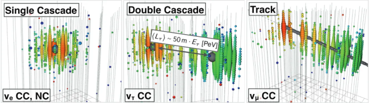
To identify the interacting neutrino’s flavor, it is of utmost importance to understand the topologies that can be created by neutrinos interacting in IceCube. Muons pass- ing through the ice leave long tracks of Cherenkov light. These track-like events are predominantly created by charged-current muon-neutrino interactions, but also stem from atmospheric muons and from the 17% of charged-current tau-neutrino interactions in which the tau decays to a muon. Cascade-like events are created by approxi- mately spherically symmetric Cherenkov emission from a single stationary light source.

Charged-current electron-neutrino interactions and the majority of charged-current tau- neutrino interactions create cascades. In addition, all neutrino flavors create cascade- like events when interacting via neutral current. These two topologies were used for the first flavor composition measurements of astrophysical neutrinos, yielding best fits of ν_e : ν_µ : ν_τ = 0.5 : 0.5 : 0.0 [32] and ν_e : ν_µ : ν_τ = 0.0 : 0.2 : 0.8 [33]. These two results are in agreement, owing to their large uncertainties, which in turn are given by the limited sensitivity to constrain three flavors with a binary topology classification. A third topology is necessary to break the degeneracy.

John Learned and Sandip Pakvasa realized that a tau with energy above 1 PeV may live long enough to travel from one optical sensor of a segmented neutrino detector to another. It can then create a so-called “double bang”, consisting of two energy depositions connected by a particle traveling with the speed of light. The tau neutrino interaction produces the first cascade-like energy deposition (or “bang”), and the tau decay produces the second “bang” if the tau does not decay into a muon. 83% of charged-current

(17)

5

tau-neutrino interactions follow this double-bang channel, but the vast majority are not distinguishable from electron-neutrino charged-current interactions due to the tau’s short lifetime. In IceCube, the spacing of the optical sensors requires a multi-PeV tau-neutrino to create a double bang that is resolvable by eye. Following the first dedicated search for high-energy tau neutrinos in IceCube [34], improved tau-neutrino detection methods have been developed, lowering the energy threshold. If the tau-neutrino interaction and subsequent tau decay happen close to a sensor, a signature called a “double pulse” can be observed [35] in that sensor, stemming from light from each of the vertices arriving at different times. The approach taken here uses a dedicated algorithm to reconstruct the topology of two causally-connected cascades [36]. This topology is called a “double cascade” and can be resolved down to several meters of tau propagation lengths. By dif- ferentiating between single cascades and double cascades, the degeneracy betweenν_eand ντ interactions is broken for high-energy neutrinos starting at energies ∼ O(100) TeV.

Classifying events into single cascades, double cascades and tracks, the contributions of each of the three flavors to the astrophysical neutrino flux can be inferred. The first analysis using the three topologies and an algorithmic topology classification based on the events’ observables was developed for IceCube’s high-energy starting events with six years of livetime. No double cascades were identified, leading to a measured flavor composition on Earth ofν_e:ν_µ:ν_τ = 0.5 : 0.5 : 0.0 and an upper limit on the astrophysical tau-neutrino flux of Φ_ν_τ(E_ν_τ)<2.95·10⁻¹⁸(E_ν_τ/100 TeV)^−2.94GeV⁻¹cm⁻²s⁻¹sr⁻¹ [37].

In the work presented in this thesis, an updated tau-neutrino search and flavor composition measurement using high-energy starting events in IceCube is presented. An additional 1.5 years of livetime are added, but also the previous analysis is improved upon. The algorithmic ternary topology classification is incorporated into the sample of high-energy starting events, an improved likelihood is used for the fitting, the treatment of systematic uncertainties is updated, and previously taken data are reprocessed following an improved detector calibration. As a result, two events are reclassified from single cascades to double cascades. The statistical treatment of the double cascade observables is improved upon, based on targeted Monte Carlo simulations for individual events. An unbiased method to evaluate sparse data in multiple dimensions is employed to properly evaluate all properties of the double cascades that are sensitive to neutrino flavor. The flavor composition is measured using a combined unbinned likelihood for the double cascades and a binned likelihood for the single cascades and tracks, in a maximum-likelihood multi-component fit.

(18)

This thesis is organized as follows. In Chapter 2, neutrino astroparticle physics is reviewed. Further, neutrino production, propagation and interaction are introduced and atmospheric and astrophysical neutrinos are described. The IceCube Neutrino Obser- vatory is described in Chapter 3, concentrating on the detector components and neutrino detection principle, as well as the Monte Carlo generation of neutrino and muon events and event reconstruction methods. Chapter 4 is dedicated to high-energy neutrino topologies and the high-energy starting event selection. In Chapter 5, the ternary topology classification and the flavor composition measurement are explained. In Chapter 6, the initial results are presented and the observables of the two found double cascades are discussed. In Chapter 7, the a posteriori analysis of the tau-neutrino candidates is presented. The targeted Monte Carlo simulation is described, and the multi-dimensional statistical treatment is developed. The final results are presented and discussed. The thesis is summarized and an outlook is given in Chapter 8.

(19)

Chapter 2

Neutrino Astroparticle Physics

Neutrinos are fundamental particles. They are stable, have no charge and almost no mass and only interact weakly. They do not get deflected or absorbed during propagation and thus can reach Earth from the distant universe. In this chapter, the basics of neutrino astroparticle physics will be reviewed. Cosmic rays are reviewed in Section 2.1, followed by a description of particle acceleration mechanisms at astrophysical sources that can lead to an observable neutrino signal on Earth in Section 2.2. What happens to neutrino flavor during neutrino propagation is explained in Section 2.3, followed by neutrino interactions at high energies in Section 2.4. Finally, in Section 2.5 the astrophysical neutrino flux and in Section 2.6 the atmospheric neutrino and muon fluxes observed by IceCube are introduced.

2.1 Cosmic Rays

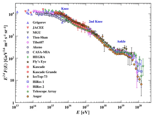
The Earth’s atmosphere is constantly hit by cosmic ray (CR) particles. These are fully ionized nuclei, about 90% protons, 9% alpha particles, and a small fraction of heavier nuclei up to iron [39]. Figure 2.1 shows the cosmic ray spectrum as measured by air shower experiments. The cosmic ray flux can be described by a power law as dN/dE ∼E^−γ over ∼10 orders of magnitude, with spectral breaks called the “knee”,

“second knee”, and “ankle” [38]:

• γ ≈2.7 for 10¹⁰ eV≲E≲E_knee∼10¹⁵⁻¹⁶ eV,

• γ ≈3.1 for E_knee ≲E≲E_ankle∼10^18.5 eV,

• γ ≈2.6 for E_ankle ≲E ≲E_cutoff ∼10^19.5 eV.

(20)

1013 10¹⁴ 10¹⁵ 10¹⁶ 10¹⁷ 10¹⁸ 10¹⁹ 10²⁰ [eV]

E 1

10 102

103

104

]-1 sr-1 s-2 m1.6 [GeVF(E)2.6 E

Grigorov JACEE MGU Tien-Shan Tibet07 Akeno CASA-MIA HEGRA Fly’s Eye Kascade Kascade Grande IceTop-73 HiRes 1 HiRes 2 Telescope Array Auger

Knee

2nd Knee

Ankle

Figure 2.1: The all-particle cosmic-ray spectrum as a function of energy per nucleus measured by air shower experiments. Figure from [38].

The “second knee” at E2nd knee∼8·10¹⁶ GeV is a subtle feature, where the spectrum slightly softens. AboveE∼10^19.5 GeV, the spectrum shows a cutoff, which could be due to the Greisen-Zatsepin-Kuzmin (GZK) cutoff, i.e. caused by interactions of ultrahigh energy cosmic rays (UHECR) with the photons of the cosmic microwave background (CMB) [40,41]. Data from the Pierre Auger Observatory indicate the composition get- ting heavier at energiesE >10¹⁸GeV [42,43], i.e. the fraction of heavy nuclei increases.

In this case, the cutoff is compatible with the effects of photodissociation of heavy nuclei.

At the lowest energies, the CR cannot penetrate the Earth’s shielding magnetic field. At about 10 GeV, about 10⁴ m⁻² s⁻¹ cosmic rays hit the atmosphere, while at the highest energies, the flux is ∼0.001 km⁻²yr⁻¹

Most of the cosmic rays are of galactic origin, some are produced by our own Sun, but at the highest energies, cosmic rays come from sources yet unknown and from beyond our galaxy. The acceleration of the cosmic rays at their sources should also lead to neutrino production, as will be explained in the next section. As CR are ionized, massive and charged particles, they get deflected during propagation through galactic and intergalac- tic magnetic fields. Therefore, neutrinos can greatly add to our understanding of cosmic rays, their origins and their production mechanisms.

(21)

2.2 Cosmic Neutrino Sources and Production Mechanisms 9 Up to energies of ∼10¹⁴ eV, cosmic rays can be measured with satellite based instru- ments. Using calorimetric detectors, the primary particle can be identified. However, above 100 TeV, the low cosmic-ray flux requires larger detector areas than can be com- fortably fit on satellite missions.

Upon impacting the atmosphere, CR collide with nuclei in the atmosphere, producing cascades of secondary particles. The processes are not unlike processes happening in beam dumps at particle accelerators on Earth. The secondary particles, mainly pions, kaons, but also heavier charmed hadrons, interact and decay, finally leading to the particles that are observed with ground-based detectors. At very high energies, cosmic rays create extensive air showers, which can be studied with large and sparse detector arrays such as the Pierre Auger Observatory [44] or the Telescope Array [45], making use of their large footprints on the ground. When high-energy charged particles from the shower reach the ground, they can be detected via the Cherenkov radiation they induce in water-filled tanks as employed by the Pierre Auger Observatory, or via scintillation light induced in scintillator surface arrays as employed by the Telescope Array. Both observatories also have detectors that capture the fluorescent light from nitrogen atoms in the atmosphere, that have been excited by charged secondary particles in the shower.

The shower development can be calculated using coupled cascade equations, describing the losses and decays of the particles in the shower [39, 46]. The cascade equations use hadronic models, which describe the interactions of the particles in the cascade.

As the hadronic models are tuned to accelerator data, they need to be extrapolated to the UHECR regime, introducing a source of systematic uncertainties. Among all the particles produced, only muons and neutrinos can reach subsurface detectors such as IceCube. It is worth mentioning that the muon multiplicity as observed by the Pierre Auger Observatory is in tension with predictions from all hadronic models [47,48].

2.2 Cosmic Neutrino Sources and Production Mechanisms

As will be described in this section, neutrino production mechanisms also lead to the production of CR and photons. Thus, when trying to explain the origin of high-energy astrophysical neutrinos, a natural start are sources known to produce high-energy photons. Many source classes have been proposed to explain the diffuse astrophysical neutrino flux observed by IceCube. However, the analyses performed with IceCube thus far only yielded upper limits on the contribution of the tested source classes to the observed neutrino flux. The observation of sources within our own galaxy in very-high-energy gamma rays makes a galactic contribution to the astrophysical neutrino flux likely. E.g.

(22)

supernova remnants (SNR) are known to be good particle accelerators. However, recent searches for correlations of IceCube neutrinos with the galactic plane or known SNR found no significant correlations and limit the galactic contribution to 14% [49], while another recent analysis revealed hints of a diffuse galactic contribution at the 2σ level [50]. Most of the diffuse astrophysical neutrino flux thus seems extragalactic in origin. A former favorite source class, Gamma-Ray-Bursts (GRBs) have been shown to contribute less than 1% to the diffuse neutrino flux [51]. Blazars, jetted Active Galactic Nuclei (AGN) with the jet pointed at Earth, were limited to a maximum of 27% of the diffuse flux [52], and supernovae to a maximum of 13% in the choked-jet scenario and 26% in the Type IIn scenario [53]. More recently, Tidal Disruption Events (TDEs) have been proposed as neutrino source candidates, also their contribution has been limited to 26%

for non-jetted and 1.3% for jetted TDEs [54]. While source classes have been proposed and subsequently disproven, and also searches for self-clustering of IceCube neutrinos have come up empty-handed¹, a search for electromagnetic counterparts to high-energy muon neutrinos has been more fruitful. On September 22, 2017, a high-energy neutrino triggered the realtime alert system [56]. The IceCube-170922A alert [57] was followed up by 16 observatories. In the 50% containment region of the neutrino, Fermi reported the blazar TXS 0506+056 to be in a flaring state [58], and MAGIC reported very high- energy gamma rays from this blazar [59]. This was the first compelling evidence for an electromagnetic counterpart to a high-energy IceCube neutrino [60]. In an independent archival search for neutrino emission from the same position, an excess of neutrinos was found which was not coincident with enhanced electromagnetic emission [61]. While the archival neutrino flare further strengthened the case of TXS 0506+056 as a neutrino source, it also poses a problem for the modeling of particle acceleration in blazars [62].

2.2.1 Particle Acceleration at Sources

As neutrinos are electrically neutral, they cannot be accelerated in sources. Instead, they are created in hadronic processes when charged particles interact with the matter or radiation fields at the sources that accelerate them. These interactions create secondary particles, whose interactions and decays create neutrinos. The primary accelerated particles eventually escape the source and may reach Earth as cosmic rays. Thus, neutrino sources are also cosmic ray sources. Finding cosmic neutrino sources able to produce neutrinos with energies up to an energy range of Exa electron Volts (EeV) would at the

1The latest point-source search for steady neutrino emission from known astrophysical sources revealed several sources that might become statistically significant in the next few years, among them TXS 0506+056. Combined, the significance of the hottest four sources, each of them with<3σsignificance, is 3.3σafter correcting for trial factors [55].

(23)

2.2 Cosmic Neutrino Sources and Production Mechanisms 11 same time yield some answers to the 100-year-old questions of the origin, the sources and the acceleration mechanisms of the highest-energy cosmic rays. While cosmic rays get deflected by magnetic fields during propagation, neutrinos and photons do not and thus point back to their sources. However, photons are more easily absorbed, and can further stem from leptonic processes, thus high-energy gamma-ray sources do not automatically need to also be cosmic ray sources.

One method to accelerate particles to very high energies at cosmic accelerators is first order Fermi acceleration, also called diffusive shock acceleration. The description below is based on [39]. If a shock propagates through a medium with a velocity u₁ ≪c, then in the frame of the shock, the gas upstream of the shock enters the shock with velocityu1, while downstream of the shock the medium is dragged behind and de- parts the shock with velocityu2. A relativistic particle can enter the shock, and scatter elastically in the shocked medium, until it leaves the shock again. By moving across the shock front twice, it can gain energy. The average gain in energy per crossing cycle is proportional to the velocity difference across the shock, and averaging over directions,

⟨∆E/E⟩=⟨δ(E)⟩ ≈4/3(u1−u2)/c. Afterncycles of crossing the shock front back and forth, the particle has the energyE_n=E₀(1 +δ)ⁿ. But the particle also has an escape probabilityPesc from the accelerating region, thus the probability to be accelerated over n cycles is (1−P_esc)ⁿ. P_esc depends on the difference in velocities between the shock front and the medium downstream,Pesc = 4u2. Thus the number of particles that can be accelerated to at least an energyEn is, using n= log(En/E0)/log(1 +δ),

N(E≥E_n)≈N₀(1−P_esc)ⁿ

=N₀(E_n/E₀)^log(1−P^esc^)/^log(1+δ)

=N₀(E_n/E₀)^1−γ,

(2.1)

whereγ = 1−log(1−P_esc)/log(1 +δ)≈1 +P_esc/δ = 1 + 3/(u₁/u₂−1) is introduced.

u1 and u2 are related by mass conservation at the shock and, assuming an ideal gas (c_p/c_v = 5/3) [63], one obtains:

u1/u2 = c_p/c_v+ 1 (c_p/c_v−1) + 2/M²

≈4(1−3/M²)

(2.2)

with the Mach number M = u1/c_s, where c_s is the speed of sound. Using the above expression, one findsγ ≈2 + 4/M². This naturally gives the differential power spectrum

(24)

10⁴ 10⁷ 10¹⁰ 10¹³ 10¹⁶ 10¹⁹ 10²² 10²⁵ Comoving size·Γ[cm]

10⁻¹⁰ 10⁻⁷ 10⁻⁴ 10⁻¹ 10² 10⁵ 10⁸ 10¹¹ 10¹⁴

MagneticFieldStrength[G]

p

Fe

HL GRB Prompt LL GRBs/TDEs

GRB/TDE Afterglow Neutron stars/

magnetars

Starburst winds

Galaxy clusters AGN Knots

AGNLobes AGNHotspots Normal galaxies

SNe Wolf-Rayet stars

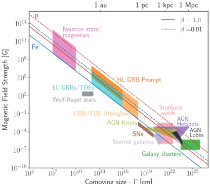
β= 1.0 β=0.01 1 au 1 pc 1 kpc 1 Mpc

Figure 2.2: Hillas diagram. Source classes are shown according to their size and magnetic ﬁeld strength. The diagonal lines indicate the threshold forBRbeyond which the source can conﬁne protons (red) and iron nuclei (blue) with energies of 10²⁰eV for shock velocitiesβ =u1/c. Sources above the diagonal line satisfy the Hillas criterion. Figure from [64].

dN/dE ≈NE⁻² for strong shocks with high Mach number, where N is now a normalization factor ﬁxed to some energy.

A source can accelerate particles while their gyroradius is much smaller than the size of the acceleration region. The maximum energy a particle can reach before it escapes the accelerating region is given by the Hillas criterion [65]:

Emax

10¹⁸eV = 3 20

u1

c Z B

G

R 10¹⁵m

(2.3) where Z is the charge of the particle, B is the source’s magnetic field, and R is the radius of the accelerating region. The so-called Hillas diagram in Figure2.2 shows source classes in terms of their radial size and magnetic field strength. Based on the radius and magnetic field considerations alone, normal galaxies such as the Milky Way cannot produce UHECR. Very large objects such as galaxy clusters or objects with extremely high magnetic fields such as neutron stars, however, can in principle confine 10²⁰ eV protons.

Fulﬁllment of the Hillas criterion alone does not guarantee cosmic-ray acceleration to

(25)

2.2 Cosmic Neutrino Sources and Production Mechanisms 13

the highest energies.

There are a few main scenarios of how to produce neutrinos from the accelerated cosmic rays at sources. In the hadronuclear scenario, cosmic rays, which are predominantly protons, interact with surrounding matter, which mostly consists of hydrogen. This is also called the pp-scenario (and if neutrons are involved, the pn-scenario). In this scenario, the interaction of high-energy cosmic rays with the target nuclei creates a particle shower, similar to the particle shower created by cosmic-ray interactions in the Earth’s atmosphere. The most abundant particles created in those showers whose decay leads to neutrino production, are charged pions, but there are also contributions from kaons and heavier mesons. In the photohadronic, or pγ-scenario, the cosmic rays interact with radiation, and pions are predominantly created via the ∆-resonance:

p+γ→∆⁺→

{ p+π⁰ (2/3 of cases),

n+π⁺ (1/3 of cases). (2.4)

The subsequent decay of neutral pions, π⁰ → 2γ, leads to the production of gamma rays and the potential observability of the source in the electromagnetic spectrum, while neutrinos are produced in the subsequent decay of the charged pions in the same way as in the pp-scenario.

Pion decay produces neutrinos via:

π^±→µ^±+⁽ν–⁾

µ, µ^±→e^±+⁽ν–⁾

µ+⁽ν–⁾

e, (2.5)

where the neutrinoνα is produced with the anti-lepton l⁺_α, and the anti-neutrino ¯να is produced with the leptonl_α⁻, conserving lepton number. Thus, the neutrino flavor ratio from pion production at source is νe : νµ : ντ = 1 : 2 : 0, where we have dropped the ν/¯ν distinction. On average, all neutrinos produced in pion decay receive ∼5% of the parent proton’s energy.

In sources with strong radiation or magnetic fields, muons interact before decaying and lose a substantial amount of their initial energy in the interactions. Thus, the resulting particles from muon decays have lower energies and do not contribute to the high- energy neutrino signal. In this so-called muon-damped production mechanism, only high-energy ν_µ and ¯ν_µ are produced, leading to a source flavor ratio of ν_e : ν_µ : ν_τ = 0 : 1 : 0. The probability for muons to interact increases with their energy, thus a gradual transition from 1 : 2 : 0→0 : 1 : 0 has been proposed [66]. Identifying such a

(26)

transition may be possible with the proposed IceCube-Gen2 facility but is out of reach in the work presented here. A muon-damped source typically is also a muon-beamed source at lower energies, where the muons pile up [67]. At the energies where muon decay completely dominates the neutrino production, the neutrinos are produced with a flavor composition of ν_e:ν_µ:ν_τ = 1 : 1 : 0.

In pγ-sources with very high magnetic field, also the pions can lose energy via radiative losses, and effectively be removed from the neutrino production. If the source is optically thin to neutrons, neutrinos are mainly produced in the decays of high-energy neutrons in the so-called neutron beam scenario [68] via

n→p+e⁻+ ¯ν_e. (2.6)

Thus, only ¯ν_e are produced at source, leading to ν_e:ν_µ:ν_τ = 1 : 0 : 0 andν : ¯ν = 0 : 1.

While the neutrino-nucleon cross-sections for anti-neutrinos are almost the same as for neutrinos at the energies at which the IceCube signal is dominated by the astrophysical neutrino component, the Glashow resonance (GR) [69] atE_ν ≈6.3 PeV can be used to probe the amount of ¯ν_e reaching IceCube. As neutrinos from neutron decay only carry

∼0.1% of the parent neutron’s energy, neutron decay only contributes to the observable neutrino flux if neutrino production from pion decay is inhibited. The parent neutrons can be produced via the ∆-resonance in Equation 2.4 or from the photodisintegration of heavy nuclei. A previous measurement of the flavor ratio disfavors the neutron decay scenario at 3.6σ [32].

Finally, the heavy mesons produced in a pγ-source may dominate the neutrino production if pions interact before decaying. This charm-production scenario [70] is equiv- alent to the prompt component of atmospheric neutrinos (see Section 2.6). The decay of charmed D and Λ_C mesons leads to the production of equal numbers of electron- and muon-neutrinos. Rare decays of D_s, D^0,± can also produce ν_τ, however, the ν_τ component always stays at least an order of magnitude below the ν_e and ν_µ components [46]. The charm-production scenario leads to a source flavor composition of νe : νµ : ντ = 1 : 1 :≤ 0.1. In general, ντ production at sources is negligible in any conceivable scenario.

At ultrahigh energies (UHE),cosmogenic neutrinoscan be produced from the decay of π⁺ created when ultrahigh-energy protons interact with photons from the (CMB). This interaction would limit the maximum energy for CR protons, known as theGZK-cutoff for UHECR protons [40,41], and produce GZK neutrinos. GZK neutrinos have not been observed yet. The decay ofπ⁰ also created in those pγCMB-interactions would produce a diffuse gamma-ray flux. Fermi-LAT measurements can be translated into an upper limit

(27)

2.3 Neutrino Propagation 15 for cosmogenic neutrinos ofE_ν²Φ_ν ≤10⁻⁸GeVcm⁻²sr⁻¹s⁻¹ at neutrino energies∼1 EeV [71]. No neutrinos have been observed in this energy range yet. Currently, the most strin- gent upper limits are obtained with IceCube’s all-flavor Extremely-High-Energy (EHE) event selection and constrain the total neutrino flux toE_ν²Φν <2·10⁻⁸GeVcm⁻²sr⁻¹s⁻¹ at neutrino energies of 1 EeV [72]. The interpretation of anomalous events reported by the ANITA collaboration as UHE neutrinos is in strong tension with limits from IceCube and the Pierre Auger observatory, see e.g. [73].

2.3 Neutrino Propagation

Neutrino oscillation describes the phenomenon of neutrinos changing flavor during propagation. The concept was not accepted yet when the first measurements of solar neutrinos were conducted at the Homestake mine. Comparing predicted neutrino interaction count rates based on calculations of the solar neutrino flux and the detector efficiency [11,74] to the observed count rate, a deficit was observed [12]. This lead to the so-called solar neutrino problem, which could only be solved decades later by the discovery of neutrino oscillations [75, 76, 77], and their resonant enhancement in matter [78, 79].

This explained the lower amount of neutrino interactions at the Homestake experiment which was only sensitive toνe. Neutrinos were long thought to be massless, and in the standard model (SM) of particle physics they are described as massless. However, neutrino oscillations can only be explained by mass differences between the three neutrinos, immediately implying at least two non-zero neutrino masses, as well as a rotation of the flavor eigenstatesαwrt. the mass eigenstatesi. So far, only upper limits on the absolute neutrino mass scale exist. A recent combination of cosmological measurements yields an upper limit to the sum of neutrino masses of∑

im_i<0.12 eV [4]. Very recently, the limits on the effective electron neutrino mass in beta decay were improved for the first time in more than two decades, and are nowm_ν <1.1 eV [5]. These masses do not have the exact same meaning, the subtleties however are not important for the analysis presented.

The cosmological measurements are more constraining, but are model-dependent, while the measurements performed using beta-decay electrons have very weak model depen- dencies, but are not as constraining. A third measurement could be obtained using neutrino-less double-beta decay, but only if this process is allowed.

2.3.1 Neutrino Masses

The origin of neutrino masses is one of the mysteries of particle physics. In the SM, there are no right-handed neutrinos, and therefore neutrinos are massless. To obtain

(28)

mass terms, one has to introduce right-handed neutrino fields, which do not participate in weak interactions. If neutrinos are Dirac particles, like quarks and charged leptons, their mass can be generated by the Higgs mechanism, too. This leads to the Dirac mass term in the Lagrangian

L^D =−ν¯_R^′ M^Dν_L^′ +h.c (2.7) where ν_R^′ are the right-handed neutrino fields. The mass terms then arise following the diagonalization of the matrix M^D,

L^D =−∑

i

m_iν¯_iν_i. (2.8)

This mechanism does not however explain the smallness of the neutrino masses, requiring Yukawa couplings orders of magnitude smaller for neutrinos than for quarks and charged leptons.

Another possibility arises if neutrinos are Majorana particles, i.e. their own antiparticles.

The Majorana Lagrangian reads

L^M =−1/2(¯ν_L^′)^cM^Mν_L^′ +h.c., (2.9) and following the diagonalization of M^M one obtains the mass terms

L^M =−1/2∑

i

m_iν¯_iν_i. (2.10)

To generate the small neutrino masses, the seesaw mechanism [80,81, 82] is employed.

As right-handed neutrinos do not participate in weak interactions, their mass is not constrained to the electroweak scale. In the seesaw mechanism, the right-handed neutrino mass term is very high and naturally suppresses the resulting neutrino mass. The Majorana nature of neutrinos would imply a violation of the total lepton number conservation, which would allow neutrinoless double-beta decay to happen.

2.3.2 Neutrino Oscillations

First devised in 1957 by Bruno Pontecorvo as neutrino–anti-neutrino oscillations [13], the idea was later developed into the three-flavor neutrino oscillation framework known today, in which neutrino change flavor, but the initially studied neutrino–anti-neutrino oscillations do not occur [14]. Neutrino flavor eigenstates α are related to the mass

(29)

2.3 Neutrino Propagation 17 eigenstatesi via a rotation matrix:

|ν_α⟩=∑

i

U_αi|ν_i⟩. (2.11)

In the standard three-flavor framework U_αi is the 3×3 Pontecorvo–Maki–Nakagawa–

Sakata (PMNS) mixing matrix [13, 14] containing three mixing angles θ_ij and one CP- violating phase δ_CP, α = {e, µ, τ}, i, j = {1,2,3}. If the masses of the neutrinos ν_i are different, their relative phases will change during propagation, leading to neutrino oscillations. The PMNS-matrix reads:

U =

⎛

⎜

⎝

1 0 0

0 c23 s23

0 −s₂₃ c₂₃

⎞

⎟

⎠·

⎛

⎜

⎝

c₁₃ 0 s₁₃e^−iδ

0 1 0

−s₁₃e^−iδ 0 c₁₃

⎞

⎟

⎠·

⎛

⎜

⎝

c₁₂ 0 s₁₂

−s12 c12 0

0 0 1

⎞

⎟

⎠P, (2.12) where the shorthand notations_ij ≡sinθ_ij andc_ij ≡cosθ_ij is used;δis theCP-violating phase; P = 13 if neutrinos are Dirac particles and P = diag(e^iα¹, e^iα²,0) with the additional Majorana phases α_1,2 if neutrinos are Majorana particles. The oscillation probability reads:

P_ν_α_→ν_β =|⟨ν_β|ν_α(L)⟩|²=∑

i,k

U_αi^∗U_βiU_αkU_βk^∗ e^i(E^k^−Eⁱ^)L (2.13)

with the baselineL. For relativistic neutrinos, we can approximate E_k =

√

p²_k+m²_k ≃ p_k+m²_k/2p_k. Setting all leading momentap_k to be equal to a common energy E for all propagating neutrino mass eigenstates yieldsE_k≃E+m²_k/2E. SubstitutingE_i−E_k=

∆m²_ik/2E with ∆m²_ik=m²_i −m²_k one arrives at

P_ν_α_→ν_β =∑

i

|U_αi|²|U_βi|²+ 2Re

⎛

⎝

∑

i,k>i

U_αi^∗ U_βi^∗U_αkU_βk^∗ eⁱ

∆m2 ikL 2E

⎞

⎠. (2.14) The second term of Equation 2.14 is the oscillation term which depends on the neutrino energyE and the traveled distance L. Evidently, in order to measure neutrino mixing parameters, it is advantageous to have a detector with a good energy resolution placed at a known distance from a source, such that maximal dip in neutrino flavor disappearance (or peak in neutrino flavor appearance) is accessible by the experiment. As neutrino sources are not monochromatic in neutrino energy, and the baselines not well defined, the oscillatory term can be ignored for extragalactic neutrinos from several sources. We

(30)

then arrive at the average oscillation probability

⟨P_ν_α_→ν_β⟩=∑

i

|U_αi|²|U_βi|². (2.15) Comparing Equation 2.15 with the values of U from Equation 2.12, one can see that the neutrino flavor composition that can be measured on Earth depends on all the mixing angles θ_ij as well as the CP-violating phase δ in addition to the initial flavor composition at the sources. By now, most of the neutrino mixing parameters have been measured by a range of dedicated experiments as well as with atmospheric neutrinos in IceCube. However, while the values of the ∆m²_ij have been measured, the sign of the mass-squared difference is only known for ∆m²₁₂. This leads to two possible mass orderings for neutrinos: In the normal ordering (NO), m₁ < m₂ < m₃, while in the inverted ordering (IO), m3 < m1 < m2. In this thesis, we use the latest three- neutrino global-fit parameters² as provided byNuFit4.1[30,83], which are summarized in Table 2.1. Note that the mass ordering and theCP−violating phaseδ are still largely unconstrained, although data indicate towardsδ ̸= 0 and the NO is preferred over IO in the latest fit. The mixing matrixU as given by NuFit4.1reads:

|U|best fit =

⎛

⎜

⎝

0.82142745 0.55031308 0.14970791 0.28831143 0.59155205 0.75295597 0.49207059 0.5892552 0.64081576

⎞

⎟

⎠, (2.16)

|U|3σ =

⎛

⎜

⎝

0.797→0.842 0.518→0.585 0.143→0.156 0.233→0.495 0.448→0.679 0.639→0.783 0.287→0.532 0.486→0.706 0.604→0.754

⎞

⎟

⎠. (2.17)

2.3.3 Expected Neutrino Flavor Composition on Earth

Due to neutrino mixing and most of the astrophysical neutrino flux observed by Ice- Cube being of extragalactic origin, the neutrino flavor composition on Earth will be different from the source flavor composition. At the energies considered for this work and with baselines exceeding the size of our galaxy, neutrino oscillations average out.

However, different source flavor compositions will lead to different Earth flavor compositions, making it possible to constrain source production mechanisms by measuring the flavor composition on Earth.

2The default version excludes atmospheric neutrino data from SuperKamiokande.

(31)

2.3 Neutrino Propagation 19

Parameter Normal Ordering (best fit) Inverted Ordering (∆χ²= 4.7)

bfp±1σ 3σrange bfp±1σ 3σrange

θ12[^◦] 33.82^+0.78_−0.76 31.61→36.27 33.82^+0.78_−0.76 31.61→36.27 θ23[^◦ 49.6^+1.0_−1.2 40.3→52.4 49.8^+1.0_−1.1 40.6→52.5 θ13[^◦] 8.61^+0.13_−0.13 8.22→8.99 8.65^+0.13_−0.13 8.27→9.03

δCP[^◦] 215⁺⁴⁰₋₂₉ 125→392 284⁺²⁷₋₂₉ 196→360

Table 2.1: Three-flavour oscillation parameters relevant to this work from fit to global data. The numbers in the 1st (2nd) column are obtained assuming NO (IO), i.e., relative to the respective local minimum. See www.nu-fit.org or [30] for all parameters.

Production Source Best fit parameters 3σmixing parameter range

scenario composition νe:νµ:ντ νe νµ ντ

pion decay 1 : 2 : 0 0.30 : 0.36 : 0.34 0.29−0.34 0.34−0.37 0.32−0.34 muon-damping 0 : 1 : 0 0.17 : 0.45 : 0.37 0.16−0.24 0.40−0.48 0.36−0.38 neutron decay 1 : 0 : 0 0.55 : 0.17 : 0.28 0.52−0.58 0.16−0.24 0.22−0.30 charm production 1 : 1 : 0 0.36 : 0.31 : 0.33 0.35−0.39 0.31−0.32 0.29−0.33

Table 2.2: Resulting flavor scenarios on Earth for given source flavor scenario, and the neutrino mixing parameters.

In Table 2.1, the resulting flavor compositions on Earth are shown for the neutrino production scenarios and source flavor compositions discussed in Section 2.2 and the oscillation parameters given in Table 2.1.

Figure 2.3 depicts the resulting flavor compositions on Earth, obtained by varying the mixing parameters from Table 2.1 within their 3σ allowed ranges. NuFit4.1 [30] pro- vides the ∆χ² values for each fit parameter and for all parameters’ two-dimensional covariances. The 3σ interval in four dimensions corresponds to an uncertainty region of

∆χ² = 16.25 in each dimension. For δ_CP, the values in ∆χ² do not reach that value, δCP is thus unconstrained. This results in a three-dimensional uncertainty problem such that the uncertainty region of interest is ∆χ² = 14.16 in each dimension and for each two-dimensional correlation. Higher-dimensional covariances are not provided, and are ignored. The resulting flavor compositions for the neutrino production mechanisms considered are shown in color. Further, the range of resulting flavor compositions for completely arbitrary source flavor compositions are shown in gray, with the region accessible only by allowing someν_τ production at source in a lighter gray shade. The filled in region thus corresponds to the maximum allowed parameter space for the neutrino flavor composition to be measured on Earth, assuming only standard mixing. As can be seen, only a small region of the full triangle is allowed. Any measurement of a flavor

(32)

Figure 2.3: Range of possible resulting flavor composition on Earth assuming mixing parameters from [30]. The filled-in region shows the total allowed parameter space if the mixing parameters are free to vary within their 3σuncertainties, and the source flavor composition is allowed to vary, with the light-gray region showing the part of the parameter space only accessible by a non-zero ν_τ fraction at the source.

composition outside of the filled-in region would point to non-standard neutrino propagation, altered e.g. by the existence of additional, sterile neutrino states, or neutrino decay. The influence of new physics on the on-Earth flavor composition is discussed in [31].

2.4 High-Energy Neutrino Interactions

Neutrinos are electrically neutral and rarely interact. They are only charged under the weak force and can only be detected indirectly, via the nuclear transformations caused by neutrino emission or capture, or, at the energies relevant for IceCube, via the particles they create in an interaction. At the energies accessible by IceCube, neutrinos interact mainly via deep inelastic scattering (DIS) with a nucleon initially bound in an atomic nucleus in the ice. Neutrinos can interact via charged-current (CC) or neutral current (NC) interactions:

(33)

2.4 High-Energy Neutrino Interactions 21

να+N →lα+X (CC) (2.18)

ν_α+N →ν_α+X (NC). (2.19)

The neutrino of flavor α = {e, µ, τ} interacts with a nucleon N bound in an atomic nucleus. The energy transferred in the process breaks apart the nucleus and leads to the creation of secondary hadrons. As these hadrons keep producing more particles as long as they have a sufficiently high energy, a high-multiplicity shower develops. The final state consists of this hadronic shower and either a neutrino (NC interaction) or a charged lepton (CC interaction) of the same flavorα. The Feynman diagrams for these interactions are shown in Figure 2.4. In a NC interaction, the neutrino scatters off a nucleon bound in a nucleus, transferring a fraction of its energy to the nucleon which creates a hadronic cascade consisting of charged and neutral hadrons. The neutrino leaves the detector following the interaction. Thus, in NC interactions, the neutrino flavor cannot be identified. In a CC interaction, the neutrino creates a charged lepton of the same flavor in addition to transferring energy to the nucleus. In CC interactions, the neutrino is destroyed, but its flavor can be identified by identifying the flavor of the final state charged lepton. The neutrino-electron cross-section can largely be neglected except for one particular case: for a ¯ν_e with an energy of E¯νe ≈M_W² /2m_e = 6.3 PeV impacting on an electron at rest, the cross-section forW−boson production is resonantly enhanced. The resonance is very narrow, and is known as the Glashow resonance [69].

After being predicted in 1960, and sought after since the beginning of data taking with IceCube, recently the first strong candidate for a GR interaction has been found [84].

The GR interaction currently is the only way to discriminate between neutrinos and anti-neutrinos in IceCube. As no GR-scale interaction was observed in the high-energy starting events (HESE) sample that this work is concerned with, we will predominantly useν to refer to neutrinos and antineutrinos.

q W^∓

p, n να

X q^′

l^±α

q Z⁰

p, n να

X q^′

να

Figure 2.4: Feynman diagrams for deep inelastic scattering interactions of neutrinos.

Left: Charged current interaction. Right: Neutral current interaction.