Renormalisation of Radiative Neutrino Masses

(1)

Renormalisation of Radiative Neutrino Masses

Moritz Ernst Lothar Platscher

München 2015

(2)

(3)

Renormierung Radiativer Neutrinomassen

Masterarbeit

an der Fakultät für Physik der

Ludwig-Maximilians-Universität München

vorgelegt von

Moritz Ernst Lothar Platscher geboren in Schwäbisch Hall

München, den 30. September 2015

(4)

Masterarbeit

am

Max-Planck-Institut für Physik (Werner-Heisenberg-Institut) Föhringer Ring 6

80805 München

eingereicht bei der Fakultät für Physik der Ludwig-Maximilians-Universität München von Moritz Ernst Lothar Platscher

am 30. September 2015

Betreut von: Dr. habil. Georg Raffelt und

Dr. Alexander Merle

(5)

Abstract

In this thesis we study the renormalisation group effects which occur in models that gener- ate neutrino masses via radiative effects, i.e. through loop-diagrams. In the present analysis the key features are illustrated by studying one particular such model, the scotogenic model proposed by Ma in 2006. This model is very simple and yet it exhibits all aspects relevant to radiative neutrino mass generation. At the same time, the methods developed are easily generalised to more involved settings. To make the results as self-contained as possible, the necessary field theoretical concepts, as well as the basics of neutrino mass generation are discussed thoroughly.

One of the key results of this work is a numerical study of the renormalisation group equations in the model under consideration. Focussing on the neutrino mixing parameters, it is found that the running can be significant in certain regions of the parameter space.

The regions of interest are identified with the aid of approximate analytical equations, which are derived explicitly. These equations describe the energy scale dependence of the leptonic mixing angles, of the phases, and of all light neutrino masses. We compute the full set of renormalisation group equations, and consider the matching of the various effective theories which result from integrating out the heavy fields. This is done perturbatively up to one-loop order. Both diagrammatic and analytic matching conditions are given and an example of how to calculate the renormalisation group equations is presented. This allows anyone to reproduce the results, making them as transparent as possible.

Finally, it can be seen from the renormalisation group equations that, in certain param-

eter regimes, there is a hierarchy-type problem in the scotogenic model which threatens

to spoil its underlying discrete symmetry. However, this symmetry is crucial to preserve

the phenomenology of the model. Since avoiding this parity problem may spoil electroweak

symmetry breaking, some tension on the parameter space is generated.

(6)

The results presented in this thesis have been obtained by the author between Octo-

ber 2014 and September 2015 at the ‘Max-Planck-Institut für Physik (Werner-Heisenberg-

Institut)’ in Munich, Germany, under the supervision of Dr. habil. Georg Raffelt and

Dr. Alexander Merle. Parts of this thesis have been published in references [1, 2].

(7)

Chapter 1 Introduction

The long standing problem of how to extend the Standard Model (SM) of elementary particle physics remains among the greatest challenges of modern science. On the one hand, collider experiments have found that the SM is a very accurate description of nature, highlighted by the discovery of the Higgs boson in 2012 [3, 4]. On the other hand, we see that the SM cannot explain certain phenomena, such as the identity of the observed Dark Matter (DM) in our Universe [5] and the origin of the small, but non-zero neutrino masses . 1 eV [6, 7].

In the absence of any signatures of new particles at colliders and no direct evidence for DM, massive neutrinos are certainly the most compelling signal of physics beyond the Standard Model (BSM). While neutrinos are predicted to be exactly massless in the SM, extending it by right-handed (RH) neutrinos requires severe fine-tuning to explain the light neutrino masses which lie many orders of magnitude below the electroweak scale. A pop- ular remedy to this fine-tuning problem is the seesaw mechanism [8–15] which introduces extremely heavy RH neutrinos. Alternatively, neutrino masses could also be generated at loop-level. This has several interesting consequences beyond the observation that the mass scale of new physics (e.g. the masses of the RH neutrinos) can be reduced to experimentally accessible values. First of all, such models usually require new fields to propagate in the loops which could be produced at colliders. Secondly, these new fields, if electrically neutral and stable against decay into lighter particles, may constitute part of the observed DM.

Furthermore, since a loop-diagram contains more couplings than a comparable tree-level diagram, we may expect that effects beyond leading order could be stronger in radiative neutrino mass models than they are e.g. in the conventional seesaw mechanism. The reason is that, unless cancellations occur, corrections to the couplings will in general add up. This could serve as an explanation for the observed neutrino mixing pattern: a mixing pattern that obeys a certain symmetry at high energies could be modified by running effects to yield the observed mixing pattern at lower energies.

On the other hand, running effects in these models can have consequences that are very

different from the aforementioned ones. Specifically, we can have settings that exhibit a

hierarchy-type problem, which is more than a mere aesthetical flaw. In such cases, one

(10)

may find that the discrete symmetry of such a model is endangered to be broken by the running masses. This can be problematic if the DM decays away quickly, and neutrino masses are generated at tree-level yielding unacceptably large values. Avoiding this parity problem can give new constraints on the parameter space of the model. However, one could argue that, if the breaking occurs at some very high energy scale, it is irrelevant as long as the low-energy phenomenology remains unaffected. We return to this discussion when we introduce the parity problem in Chapter 6. It will become clear that, even if this point of view is taken, significant constraints can arise.

To illustrate these rather generic remarks, we use the so-called scotogenic model as our benchmark model, which was proposed in Ref. [16]. Throughout this thesis we work in natural units, where ~ = c = 1, and use a metric signature (+, −, −, −). Unless indicated otherwise, we assume summation over repeated indices. Vectors in three-dimensional Eu- clidean space are indicated by bold-face symbols, while four-vectors in Minkowski space are written in italics.

The structure of this thesis is the following: in Chapter 2 we review the basic field theoretical methods employed throughout this work. In the subsequent Chapter 3 some of the mechanisms which could be responsible for the generation of neutrino masses are discussed. The main results of our work are outlined in Chapter 4, where we discuss the necessary steps to arrive at the running neutrino masses, leptonic mixing angles, and phases. Subsequently, we apply these findings to illustrate the running of the neutrino mixing parameters in Chapter 5, and in Chapter 6 we finally highlight the parity problem.

A summary of the results is given in Chapter 7. Technical details can be found in the

appendices.

(11)

Chapter 2 Theoretical Preliminaries

In this chapter we discuss some of the theoretical concepts which will be needed throughout this work and go beyond introductory courses on quantum field theory (QFT). We begin with an introduction to regularisation, renormalisation, and an overview of some relevant renormalisation group methods in Sec. 2.1. Subsequently, we study effective field theories (EFTs) in Sec. 2.2. Finally, Sec. 2.3 is dedicated to the concept of Majorana fermions and lepton number violating interactions. These self-conjugate fermions are often a source of confusion since they are usually not covered in standard courses on QFT. Any unacquainted reader will hopefully benefit from this discussion.

2.1 Regularisation and Renormalisation

To the best of our knowledge, Nature is described on a fundamental level by interacting QFTs. However, as soon as interactions are inserted into the Lagrangian, no closed solu- tions can be found in general. Hence, we are restricted to the use of perturbation theory.

The leading order contributions, often at tree-level, usually yield good first impressions of a given scattering process. Going beyond tree-level calculations, however, one may immedi- ately encounter divergent expressions. Such loop-level expressions involve integrations over momenta, which are not fixed by momentum conservation, and which may not converge in all cases. This makes the assumption of a perturbative expansion seem entirely wrong, a fact which even some of the founding fathers of QFT disapproved of (see e.g. Ref. [17]).

The renormalisation group method enables us to tackle this issue self-consistently and extract predictions concerning the running of coupling ‘constants’ and masses (i.e. their dependence on the energy scale under consideration). This curious behaviour has in fact been verified experimentally, e.g. by measuring the running of the QCD fine structure constant [18].

To illustrate the running, we consider the following toy theory of a real and massive spin-0 boson with quartic self-interactions:

L = 1

2 (∂

_µ

φ) (∂

^µ

φ) − m

²

2 φ

²

− λ

4! φ

⁴

. (2.1)

(12)

Even though this toy model is a highly simplified example, it will clarify the most important concepts which generalise straight-forwardly to more complicated and realistic models like those discussed in later chapters.

2.1.1 Dimensional Regularisation

In order to make sense of a perturbation series with divergent coefficients, we first need to find a way of assigning a finite value to the diverging integrals. To this end, we have several options. For example, the one-loop correction to the two-point function in the above theory would be quadratically divergent (

¹₂

is a symmetry factor):

− iΣ

⁽¹⁾

=

.

= 1 2 (−iλ)

Z d

⁴

k (2π)

⁴

i

k

²

− m

²

+ iη ∼ Z

Λ

0

dk k

³

k

²

∼ Λ

²

, (2.2)

where Λ is a momentum cut-off. In principle, such a cut-off is a valid regulator. However, it introduces further subtleties, because it can destroy gauge invariance [19].

The most convenient option for our purposes is dimensional regularisation. Here, we use an arbitrary dimension d of space-time such that the integral converges to a well- defined value which is analytically continued even to non-integer dimensions d ≡ 4 − ε [20].

Considering the above integral in d 6= 4 dimensions, we have:

− iΣ

⁽¹⁾

→ −iΣ

⁽¹⁾_d

= λ 2

Z d

^d

k (2π)

^d

1 k

²

− m

²

+ iη , (2.3)

which converges for sufficiently small d, as power counting reveals. This integral can be calculated using the following steps:

1. Rotate the k

⁰

-integration contour to go from −i∞ to +i∞. This so-called Wick rotation is shown schematically in Fig. 2.1 and makes explicit use of the pole structure in the k

⁰

-plane [21, 22].

2. Define new integration variables ik

_E⁰

≡ k

⁰

and k

_E

≡ k, i.e. go to Euclidean space.

3. Perform the integral in d = 4 − ε dimensions and expand in powers of ε. This allows one to isolate the divergences as poles at ε = 0.

4. Check whether coupling constants acquire a mass dimension in d 6= 4 dimensions.

For example, the Lagrangian in Eq. (2.1) has a mass dimension d. From its kinetic or

mass terms it follows that the field has a mass dimension [φ] = (d − 2)/2. Applying

this to the interaction, we see that [λ] = ε. We can then introduce λ

⁰

= µ

^ε

λ as the

actual coupling in the Lagrangian, where µ is some arbitrary mass scale and λ is

dimensionless.

(13)

2.1 Regularisation and Renormalisation 5

Re k

⁰

Im k

⁰

√ k

²

+ m

²

− iη

− √

k

²

+ m

²

+ iη

Figure 2.1:

Wick rotation of the

k⁰

-integration. See also [22], where a similar drawing is shown.

Performing the above steps, one finds:

−iΣ

⁽¹⁾_d

= µ

^ε

λ 2

Z d

^d

k (2π)

^d

1 k

²

− m

²

+ iη = i µ

^ε

λ 2

Z d

^d

k

_E

(2π)

^d

1 −k

²_E

− m

²

= −i µ

^ε

λ 2

1 (2π)

^d

Z

d

^d−1

Ω Z

∞

0

dk k

^d−1

k

²

+ m

²

= i λ 32π

²

m

²

2 ε + 1 − γ

E

− log (4π) + log µ

²

m

²

+ O (ε)

,

(2.4)

where R

d

^d−1

Ω is the the surface area of a d-dimensional unit sphere and γ

_E

≈ 0.57722 is the Euler-Mascheroni constant. This expression is an analytic function of ε with a simple pole at ε = 0 (d = 4). For all practical purposes, it is sufficient to follow this approach to dimensional regularisation. In some cases, however, one has to be cautious. In Ref. [20], the authors show by a more formal definition of dimensional regularisation that the integral of any polynomial of momenta vanishes:

Z d

^d

k

(2π)

^d

k

²

α

= 0, for α ∈ R. (2.5)

If no care is taken, following the above calculation for m = 0, we can arrive at a result that has a pole at d = 2 and is finite in the limit ε → 0. Alternatively, we can see that if we set m = 0 in Eq. (2.4), we get Σ

⁽¹⁾_d

= 0. This ambiguity occurs when external scales are absent. It can be lifted by either following the authors of Ref. [20], or by taking Eq. (2.5) as a definition.

2.1.2 Renormalisation

The next step in the renormalisation programme is to remove the singularity at d = 4 from

Eq. (2.4), so that we may take the limit d → 4. The prescription according to which this

(14)

is done is called the renormalisation scheme. To understand the physical implications of choosing a particular renormalisation scheme, let us consider an example. Following the standard procedure and decomposing the full propagator into 1-particle irreducible (1PI)

¹

contributions, we obtain at the one-loop level [22–24]:

= + . + . . + · · · S(p

²

) = i

p

²

− m

²

+ i

p

²

− m

²

−iΣ

⁽¹⁾

i p

²

− m

²

+

+ i

p

²

− m

²

−iΣ

⁽¹⁾

i

p

²

− m

²

−iΣ

⁽¹⁾

i

p

²

− m

²

+ · · ·

= i

p

²

− m

²

− Σ

⁽¹⁾

`−loop

− −−− → i

p

²

− m

²

− (Σ

⁽¹⁾

+ Σ

⁽²⁾

+ · · · ) , (2.6) with Σ

^(`)

the 1PI `-loop two-point function with amputated external legs. From this equation it is apparent that we can absorb the divergences in Σ

^(`)

by redefining our fields and parameters in the Lagrangian (2.1). Namely, we replace the bare fields and parameters by renormalised ones:

φ ↔ φ

_B

≡ Z

¹²

φ

_R

, (2.7a)

m

²

↔ m

²_B

≡ Z

⁻¹

m

²_R

+ δm

²

, (2.7b)

λ ↔ λ

_B

≡ Z

⁻²

µ

^ε

Z

_λ

λ

_R

. (2.7c)

Note that the bare quantities are precisely those of the Lagrangian in Eq. (2.1). The subscripts B and R are merely added in this section to avoid any confusion between bare and renormalised quantities. One can think of the quantities Z , δm

²

and Z

λ

as originating from the self-interactions of a freely propagating particle. Thus, they contain all the divergences, while any renormalised quantity is finite. In any experiment, we will measure the renormalised coupling, mass, etc. of a field, which already contain all quantum corrections and are finite.

By splitting Z = 1 + δZ and Z

_λ

= 1 + δλ, we arrive at a renormalised Lagrangian which is the sum of the original Lagrangian and a counter term Lagrangian. Note that both parts are written in terms of the measurable and finite quantities m

_R

and λ

_R

:

L = L

_R

+ L

_ct

= 1

2 (∂

_µ

φ

_R

) (∂

^µ

φ

_R

) − m

²_R

2 φ

²_R

− µ

^ε

λ

_R

4! φ

⁴_R

+ + 1

2 δZ (∂

_µ

φ

_R

) (∂

^µ

φ

_R

) − δm

²

2 φ

²_R

− µ

^ε

δλ λ

_R

4! φ

⁴_R

.

(2.8)

Repeating the above calculation in Eq. (2.3) for the renormalised theory, we obtain the renormalised two-point function:

Σ

⁽¹⁾_R

= −iΣ

⁽¹⁾_d

+ i p

²

δZ − δm

²

. (2.9)

1Such a diagram isnot disconnected if any internal line is cut.

(15)

2.1 Regularisation and Renormalisation 7 We can now specify a renormalisation scheme, i.e. the way in which we subtract the pole at ε = 0 from Eq. (2.4). This subtraction is not unique and in fact this arbitrariness is what leads to the renormalisation group.

²

One option is to specify that the renormalised parameters in the Lagrangian correspond to the physically measured ones, in our case the physical mass of a particle. A possible set of renormalisation conditions on the 1PI two point function G

⁽²⁾_R

≡ Σ

⁽¹⁾_R

+ Σ

⁽²⁾_R

+ · · · would be:

G

⁽²⁾_R

p²=m²_R

= 0, and (2.10a)

d

d (p

²

) G

⁽²⁾_R

p²=m²_R

= 0, (2.10b)

which needs to be fulfilled to all orders in perturbation theory. This leaves the physical mass of the particles, i.e. the location of the pole, at m

_R

. The second condition fixes the residue of the pole in the propagator to 1, as can be verified by considering Eq. (2.6).

Imposing Eqs. (2.10a) and (2.10b) at one-loop order yields:

³

δZ

_OS

= 0 and δm

²_OS

= −Σ

⁽¹⁾_d

p

²

= µ

²

= m

²_R

= λ

_R

32π

²

m

²_R

2 ε + 1 − γ

_E

− log (4π)

. (2.11) This is known as the on-shell (OS) scheme.

Alternatively, we can use the counter terms more economically and subtract the divergent parts only. This renormalisation scheme is the so-called minimal subtraction (MS) scheme.

In the MS scheme, we find that again δZ

MS

= 0 and:

δm

²_MS

= λ

32π

²

m

²_R

2 ε . (2.12)

However, one should realise that now m

R

is not necessarily the physical mass of a particle, since the full propagator’s pole structure is modified:

S

_MS⁻¹

(p

²

, µ

²

) = p

²

− m

²_R

1 − λ

_R

32π

²

1 − γ

_E

− log (4π) + log µ

²

m

²_R

+ O λ

²_R

(4π)

⁴

. (2.13) A modified version of this is the MS scheme, where the constant factor [1 − γ

_E

− log (4π)] is also subtracted.

⁴

In principle, we can subtract an arbitrary dimensionless constant yielding an MS-like scheme where the various renormalisation constants take the form:

δZ

k

= X

i≥1

δZ

_k⁽ⁱ⁾

˜

ε

ⁱ

. (2.14)

The common feature of the MS-like schemes is that ε ˜ is a dimensionless constant which diverges in the limit d → 4, and the δZ

_k⁽ⁱ⁾

are independent of ε. ˜

2In many cases these ambiguities form a group algebra, but sometimes no inverse transformation exists (cf. the block spin analogy [25]) such that they only form a semi-group.

3It is a coincidence of pureφ⁴ theory thatΣ⁽¹⁾_d is independent ofp² and henceδZ= 0.

4In this very simple example, where the self-energy is independent of external momenta, the MS scheme coincides with the OS scheme.

(16)

A theory in which all divergences occurring at any loop order can be absorbed into a finite number of counter terms, which are obtained by redefining the existing parameters, is called a renormalisable theory. By counting powers of loop momenta, one can show that a necessary condition for a theory to be renormalisable is that it contains only couplings that have positive or no mass dimension [24, 26]. In contrast, those theories where the couplings have inverse mass dimensionality are non-renormalisable. Non-renormalisable theories are theories in which one would need infinitely many counter terms to cancel all divergences that may occur.

A full proof of renormalisability is much more involved since one has to show that all correlation functions can be made finite at any loop order by a finite number of counter terms. See Refs. [27–29] for examples of such proofs.

2.1.3 The Renormalisation Group and the Callan-Symanzik Equa- tion

As we have seen in the previous section, there is some freedom in how we subtract the divergences and absorb them into the counter terms. In addition, even after choosing a renormalisation scheme, say MS, the mass parameter µ, which has been introduced for dimensional reasons, is still present in our final result in Eq. (2.13). However, the bare Lagrangian is independent of µ and thereby correlation functions of bare fields do not depend on µ. Moreover, we can use Eqs. (2.7) and (2.8) to express a bare correlation function in terms of renormalised quantities:

G

⁽ⁿ⁾_B

{x

_i

}

_1≤i≤n

; λ

_B

, m

_B

≡ h0| T φ

_B

(x

₁

)φ

_B

(x

₂

) · · · φ

_B

(x

_n

) |0i

= Z

ⁿ²

(µ) h0| T φ

R

(x

1

)φ

R

(x

2

) · · · φ

R

(x

n

) |0i

= Z

ⁿ²

(µ) G

⁽ⁿ⁾_R

{x

_i

}

_1≤i≤n

; λ

_R

, m

_R

, µ

, (2.15)

where G

⁽ⁿ⁾_R

is the renormalised n-point correlation function and T is the time ordering operator. The fact that bare correlation functions do not depend on µ is parametrised by the so-called Callan-Symanzik equation [30–32]:

µ d

dµ G

⁽ⁿ⁾_B

({x

_i

} ; λ

_B

, m

_B

) = 0, from which it follows that

µ ∂

∂µ + β

_λ

∂

∂λ

_R

− γ

_m

m

_R

∂

∂m

_R

+ nγ

G

⁽ⁿ⁾_R

({x

_i

} ; λ

_R

, m

_R

, µ) = 0. (2.16) Here, β

_λ

≡ µ

^dλ_dµ^R

is the so-called β-function or renormalisation group equation (RGE) of the running coupling λ

_R

(µ). The functions γ

_m

≡ −

_m^µ

R

dmR

dµ

and γ ≡

_2Z^µ ^dZ_dµ

are the anomalous dimensions of the mass m

_R

and the field φ

_R

, respectively.

The above equation states that any change in the renormalisation scheme, which amounts

to a finite and potentially µ-dependent shift of the counter terms, is compensated by an

appropriate change in the scale µ [27]. For example, from Eqs. (2.11) and (2.12) we see

that δm

²_OS

= δm

²_MS

+

_32π^λ^R2

m

²_R

[1 − γ

_E

− log (4π)]. This removes some of the arbitrariness

in choosing a renormalisation scheme by relating the scheme to the scale µ.

(17)

2.1 Regularisation and Renormalisation 9 The meaning of µ. In more involved calculations than the simple example of a real scalar field, one usually encounters logarithms of the type log

p² µ²

, where p is an external momentum. To minimise potentially large logarithms due to a poor choice of the renormal- isation scale µ, one chooses µ ∼ E, where E is a typical energy scale for the process, e.g. it could be the centre of mass energy √

s in a scattering process. Thus, µ is to be identified with the energy scale under consideration. In the following Sec. 2.2, an example for such a large logarithm, that can be tamed by a suitable choice of µ, can be found. Before turning to this discussion, however, we will demonstrate how to calculate β-functions in practice.

Calculating β-functions. The MS scheme is a so-called mass-independent scheme be- cause the subtraction of the ε

⁻¹

-pole is not specified at a certain energy scale. As a consequence, the counter terms depend only implicitly on the scale µ. This requires some care when calculating β-functions. The following derivation closely follows Refs. [33, 34].

Take some bare coupling or mass Q

_B

, for which it is true that:

µ d

dµ Q

_B

= 0. (2.17)

In general, there is a relation:

Q

_B

= Z

_Q

µ

^D^Q^ε

(Q + δQ), (2.18)

where Z

_Q

contains all contributions stemming from wave function renormalisation con- stants Z [cf. Eq. (2.7a)]. Furthermore, D

_Q

is the additional mass dimensionality the quantity acquires in d = 4 − ε dimensions. Note that, unless there is some symmetry at work, we should not expect Q to be renormalised multiplicatively, which would imply δQ ∝ Q. Thus, in order to cover the most general case possible, we have introduced δQ as an additive correction. In case Q is indeed renormalised multiplicatively, we will simply find δQ ∝ Q. Inserting Eq. (2.18) into Eq. (2.17), we find:

0 = µ d dµ Q

_B

=

µ dZ

_Q

dµ (Q + δQ) + D

_Q

ε Z

_Q

(Q + δQ) + Z

_Q

β

_Q

+ µ dδQ dµ

µ

^D^Q^ε

, (2.19) where β

_Q

≡ µ

^dQ_dµ

is the β-function we aim at. The chain rule can be used to eliminate the factors

^dδZ_dµ^Q

and

^dδQ_dµ

in favour of beta functions of Q and other quantities. These are represented by V

_i

and Eq. (2.19) can be expressed as (a sum over i is implied):

0 = dδZ

_Q

dQ β

_Q

(Q + δQ) + dδZ

_Q

dV

_i

β

_V_i

(Q + δQ) + D

_Q

ε Z

_Q

(Q + δQ)+

+ Z

Q

β

Q

+ Z

Q

dδQ

dQ β

Q

+ dδQ dV

_i

β

Vi

.

(2.20)

At N -loop order, our renormalisation constants will have received contributions from all

loop orders ≤ N . In a mass-independent subtraction scheme they will most generally take

(18)

the form given in Eq. (2.14):

Z

_Q

= 1 +

N

X

i=1

δZ

_Q⁽ⁱ⁾

ε

ⁱ

, δQ =

N

X

i=1

δQ

⁽ⁱ⁾

ε

ⁱ

, and δV

_i

=

N

X

j=1

δV

_i^(j)

ε

^j

. (2.21) Additionally, β

_Q

must be finite because it is a function of finite renormalised quantities.

Therefore, we can try the ansatz:

β

_Q/V_i

= β

_Q/V⁽⁰⁾

i

+ εβ

_Q/V⁽¹⁾

i

+ ε

²

β

_Q/V⁽²⁾

i

+ · · · + ε

^m

β

_Q/V^(m)

i

−−→

ε→0

β

_Q/V⁽⁰⁾

i

, (2.22)

for some integer m which is not necessarily affiliated with the loop order N . Plugging Eqs. (2.21) and (2.22) into (2.20) and equating coefficients, it is apparent that Z

_Q

β

_Q

gives rise to the only O (ε

^m

) term. It follows that β

_Q/V⁽ⁿ⁾

i

= 0 for n ≥ 2.

At order ε

¹

, we find:

β

_Q⁽¹⁾

= −D

_Q

Q and similarly β

_V⁽¹⁾

i

= −D

_V_i

V

_i

(no sum). (2.23) At order ε

⁰

, Eq. (2.20) reads:

0 = dδZ

_Q⁽¹⁾

dQ β

_Q⁽¹⁾

Q + dδZ

_Q⁽¹⁾

dV

i

β

_V⁽¹⁾

i

Q + D

_Q

δZ

_Q⁽¹⁾

Q + D

_Q

δQ

⁽¹⁾

+ + β

_Q⁽⁰⁾

+ β

_Q⁽¹⁾

δZ

_Q⁽¹⁾

+ dδQ

⁽¹⁾

dQ β

_Q⁽¹⁾

+ dδQ

⁽¹⁾

dV

_i

β

_V⁽¹⁾

i

,

(2.24)

which we can solve for β

_Q⁽⁰⁾

by using Eq. (2.23). Thereby, the beta function in d = 4 is given by:

β

_Q⁽⁰⁾

= D

_Q

dδQ

⁽¹⁾

dQ Q + D

_V_i

dδQ

⁽¹⁾

dV

_i

V

_i

− D

_Q

δQ

⁽¹⁾

+ Q

"

D

_Q

dδZ

_Q⁽¹⁾

dQ Q + D

_V_i

dδZ

_Q⁽¹⁾

dV

_i

V

_i

#

. (2.25) This is the final result for the calculation of β-functions in MS-like renormalisation schemes.

It is easily generalised to couplings with tensorial structure, e.g. a Yukawa matrix. The derivations that can be found in Refs. [33, 34] give explicit formulae for such cases. For the concrete case of a matrix-valued quantity Y one obtains, in analogy to Eq. (2.18):

Y

_B

= µ

^D^Y^ε

Z

_L

(Y + δY ) Z

_R

. (2.26) Repeating the above computation yields:

β

_Y ^ε→0

= D

_Y

dδY

⁽¹⁾

dY

ij

Y

_ij

+ D

_V_i

dδY

⁽¹⁾

dV

i

V

_i

− D

_Y

δY

⁽¹⁾

+ +

"

D

_Y

dδZ

_L⁽¹⁾

dY

_ij

Y

_ij

+ D

_V_i

dδZ

_L⁽¹⁾

dV

_i

V

_i

# Y + Y

"

D

_Y

dδZ

_R⁽¹⁾

dY

_ij

Y

_ij

+ D

_V_i

dδZ

_R⁽¹⁾

dV

_i

V

_i

# .

(2.27)

Note that we have assumed a treatment up to N -loop order, but only δQ

⁽¹⁾

and δZ

_Q⁽¹⁾

enter

Eq. (2.27). Hence, only the ε

⁻¹

contributions to the counter terms are relevant. This fact

can facilitate higher loop calculations significantly.

(19)

2.2 Effective Field Theories 11

iΠ

^νρ_R

= i(p

²

g

^νρ

− p

^ν

p

^ρ

) Π

_R

= ρ . . ^ν

e

+ ρ ν

δZ

_A

Figure 2.2:

One-loop QED vacuum polarisation and counter term.

2.2 Effective Field Theories

The decoupling of high-energy degrees of freedom is a well-established paradigm throughout the various fields of physics. Examples are easily found: we do not consider the parton structure of the proton when solving the hydrogen atom’s Schrödinger equation. Similarly, we are not interested in the quantum mechanical (QM) energy levels of an individual atom if we study the mechanical properties of a macroscopic solid state system. The crucial observation is that for sufficiently small energy scales the low-energy effective theory is a good approximation of the full theory, which we may not even know. But even if the full theory is known, the approximation can facilitate computations, e.g. at non-relativistic velocities classical mechanics is a good approximation of special or even general relativity and much easier to handle.

2.2.1 The Decoupling Theorem

In QFT, the first proof of the decoupling of heavy fields at energies much smaller than their masses was given in Ref. [35]. The authors have made use of two facts: firstly, for energies much below the mass m of the heavy field, no heavy external states can be produced. Secondly, due to the structure of the propagators [(p

²

− m

²

)

⁻¹

for bosons and

/ p − m

−1

for fermions], internal lines of heavy fields are accompanied by a suppression of the form ‘energy scale over heavy mass’, e.g. (p

²

− m

²

)

⁻¹

=

_m⁻¹2

P

n

p² m²

n

, which is valid for p

²

< m

²

. Therefore, the low-energy effects from the heavy field can be approximated arbitrarily well by truncating the geometric series at a desired order.

To prove the decoupling theorem, a renormalisation scheme needs to be found such that the decoupling is manifest even after renormalisation [27]. Without going into the details of the proof, we illustrate that this is not straight-forward, especially in mass-independent renormalisation schemes such as MS and MS.

In QED, the one-loop vacuum polarisation, i.e. the photon self-energy, is given by the left diagram shown in Fig. 2.2. Using dimensional regularisation, we obtain [22]:

Π(p

²

, m

²

, µ

²

) = − 2α π

Z

1 0

dx x(x − 1) 2

ε − γ

_E

+ log (4π) + log

µ

²

m

²

− x(1 − x)p

²

,

(2.28)

(20)

where α =

_4π^e²

is the fine structure constant and m the electron mass.

In the OS renormalisation scheme, we impose that the divergence in the self-energy is cancelled by its counter term δZ

_A

at the physical photon mass, i.e. at p

²

= 0. This makes the OS scheme mass-dependent. Thereby, we obtain the OS renormalised vacuum polarisation:

Π

^(OS)_R

(p

²

, m

²

, µ

²

) = − 2α π

Z

1 0

dx x(x − 1) log

m

²

m

²

− x(1 − x)p

²

| {z }

=x(1−x)^p²

m2+O

p4 m4

. (2.29)

In this expression the µ-dependence has dropped out and the expansion of the logarithm is valid for p

²

< m

²

. Therefore, at energies much below the electron mass, the decoupling of the electrons is taken care off automatically in the OS scheme. However, in the opposite limit, p

²

m

²

, it contains a large logarithm ∼ log

m² p²

, as anticipated in the previous section.

⁵

In the MS scheme, in contrast, we subtract only the divergent part (plus constants) from the vacuum polarisation. This way we get:

Π

^(MS)_R

(p

²

, m

²

, µ

²

) = − 2α π

Z

1 0

dx x(x − 1) log

µ

²

m

²

− x(1 − x)p

²

| {z }

=−log

m2

µ2−x(1−x)^p²

µ2

. (2.30)

Choosing µ

²

∼ p

²

, we encounter for small energy scales a large logarithm ∼ log

p² m²

in the expression (2.30). This means that perturbation theory cannot be trusted in the limit p

²

m

²

because the electrons are not properly decoupled in this renormalisation scheme.

At high energies (p

²

m

²

), in contrast, this logarithm is small and perturbation theory is applicable.

This illustrates that the use of perturbation theory in QFT requires some caution when considering low-energy effective theories. Also, this example emphasises the intimate rela- tion between EFTs and renormalisation.

To avoid such large logarithms at low energies in mass-independent renormalisation schemes, we make use of the decoupling theorem. According to its proof a renormal- isation scheme must exist in which decoupling is manifest. At the same time, we can switch between the renormalisation schemes at will, because any change in the renormal- isation prescription can be compensated by appropriately changing the renormalisation scale. Thus, we may decouple heavy particles at energy scales far below their masses by hand. This procedure is called integrating out the heavy degrees of freedom and we will describe the procedure in the following subsection.

⁶

5In principle, the issue of a large logarithm in this limit can be cured by imposing the cancellation to occur atp²= Λ². Then the scale Λtakes a role similar to that ofµin the MSscheme.

6This terminology originates from the path integral formalism and in our approach, we should speak of matching instead.

(21)

2.2 Effective Field Theories 13 e(p

₂

)

u(p

₁

)

ν(p

₄

)

d(p

₃

)

. .

W

^q ⁼^p²⁻^p⁴

q²M_W²

−−−−−→

e(p

₂

)

u(p

₁

)

ν(p

₄

)

d(p

₃

)

Figure 2.3:

Electron capture

pe→nν.

2.2.2 Effective Operators and Matching

A well-known example for a low-energy EFT is the Fermi theory of weak interactions.

The process shown in Fig. 2.3 (left diagram) is mediated by a massive W -boson. For energies well below the W mass M

_W

, we can follow the above reasoning and expand the W -propagator in powers of

q² M_W²

. This procedure yields an effective four-fermion interaction (spin indices are suppressed):

u(p

₄

) i

√ 2 gγ

^µ

P

_L

u(p

₂

) −ig

_µν

q

²

− M

_W²

u(p

₃

) i

√ 2 gγ

^ν

P

_L

u(p

₁

)

q²M_W²

−−−−−→ −i g

²

2M

_W²

u(p

₄

)γ

^µ

P

_L

u(p

₂

)u(p

₃

)γ

_µ

P

_L

u(p

₁

) + O q

²

M

_W²

.

(2.31)

Thus, expanding the W -propagator for small energies has decoupled the W -boson by con- tracting the internal line into an effective vertex (cf. Fig. 2.3, right diagram). The effective coupling constant is given by the Fermi constant G

_F

=

√2g²

8M_W²

, which is suppressed by the mass scale M

_W

. This amplitude can be obtained from the following interaction Lagrangian:

L

_Fermi

= G

_F

√ 2

νγ

^µ

1 − γ

⁵

e dγ

_µ

1 − γ

⁵

u

+ h.c. (2.32)

Note that, even though this interaction is non-renormalisable, it is only valid for energies up to approximately M

_W

. Thus, for energies larger than M

_W

we must turn to the ultraviolet (UV) completion – the Standard Model which is renormalisable!

We can continue the expansion in

q²

M_W²

and eventually obtain an infinite tower of non-renormalisable effective interactions [36]:

L

_eff

= X

n≥5

C

_n

M

_Wⁿ⁻⁴

O

⁽ⁿ⁾

, (2.33)

(22)

where the operators O

⁽ⁿ⁾

have a mass dimension n. Note that not all of them have to be be realised, e.g. the operator in L

_Fermi

contributes to O

⁽⁶⁾

, while O

⁽⁵⁾

= 0 in the above example.

This approach, where the UV completion of a theory is known and higher dimensional operators can be related to its couplings, is called top-down. In practice, rather than expanding propagators, one includes terms of the form Eq. (2.33) up to a desired order and matches the couplings C

_n

to those of the UV completion, e.g. diagrammatically [37].

Of course one can reverse this approach, yielding the so-called bottom-up approach, which does not require the knowledge of any UV theory. We simply include all possible non-renormalisable interaction terms, which should respect the theory’s symmetries, up to a desired order in Λ

⁻¹

where Λ represents the scale of new physics. Again, not all of these operators need to be realised in the UV theory, as we have seen above. The down-side of this approach is that, in order to perform loop calculations, more and more effective operators are needed to have enough counter terms that can cancel the occurring divergences due to their non-renormalisable nature. Nevertheless, the bottom-up approach allows one to gain some insight into physics beyond the low-energy EFT. We illustrate this by treating the SM as an EFT in the bottom-up approach. Including effective operators up to a mass dimension D = 5, we find that only one such operator is allowed by the SM gauge symmetry, the so- called Weinberg operator [38]:

L

D=5

= 1

4 κ

ij

`

^c_L^a_i

ε

ab

φ

^b

`

Le

j

ε

ef

φ

^f

+ h.c. (2.34) In this expression `

_L

is the left-chiral lepton doublet and φ is the Higgs doublet. Dimen- sional analysis shows that κ is of mass dimension (−1) and can be expressed in terms of dimensionless couplings y

_ij

and the scale Λ: κ

_ij

=

^y_Λ^ij

. From the point of view of neu- trino physics, the most interesting feature of the Weinberg operator is that it gives rise to Majorana neutrino masses as the Higgs acquires a vacuum expectation value (VEV):

1 4 κ

_ij

`

^c_L^a_i

ε

_ab

φ

^b

`

_L^e_j

ε

_ef

φ

^f

+ h.c.

^hφi=(0,v)

T

−−−−−−→ v

²

4Λ y

_ij

| {z }

≡¹₂(Mν)ij

ν

_Li^c

ν

_Lj

+ h.c. (2.35)

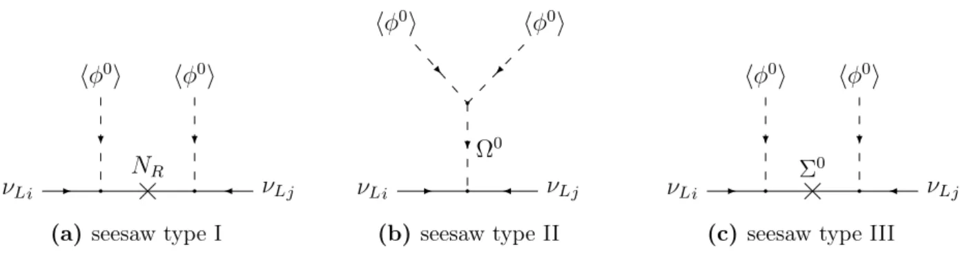
It is evident that a natural explanation for the smallness of neutrino masses is a large scale Λ, which is the basic idea of the seesaw mechanism: the larger the scale of new physics Λ is, the smaller the neutrino mass scale. In Chapter 3 we will study potential UV completions of the SM that realise the Weinberg operator.

To summarise, by a bottom-up treatment of the SM as an EFT, we have gained in-

sight into some features of possible UV completions: we expect (light) neutrino masses as

verified experimentally (see next chapter) and lepton number violation through the (Ma-

jorana) neutrinos’ interactions (cf. next section). Finally, we should see some new particles

appearing around a mass scale Λ. However, in case the Weinberg operator is not realised

in the UV completion of the SM, these observations can be altered significantly.

(23)

2.3 Majorana Fermions 15

2.3 Majorana Fermions

In any course on QFT the first concept that is introduced is the real scalar field, followed by the complex scalar field and eventually the Dirac field – a complex field describing particles of spin

¹

/

2

. The natural question to ask is whether there is a real solution to the Dirac equation, just as there is a real solution to the Klein-Gordon equation. Thus, we need to verify whether we can impose the additional reality condition ψ = ψ

^∗

on a fermion field ψ which satisfies the Dirac equation,

(iγ

^µ

∂

_µ

− m) ψ(x) ≡ (i / ∂ − m)ψ(x) = 0. (2.36) Here, the γ

^µ

are the so-called Dirac matrices satisfying the anti-commutation relations

{γ

^µ

, γ

^ν

} ≡ γ

^µ

γ

^ν

+ γ

^ν

γ

^µ

= 2g

^µν

1 (Clifford algebra), (2.37) where 1 is the identity matrix. To find the equation of motion ψ

^∗

obeys, we take the complex conjugate of Eq. (2.36). Hence, we see that unless the Dirac matrices are purely imaginary, i.e. γ

^µ∗

= −γ

^µ

, we cannot impose ψ = ψ

^∗

[39]. Clearly, this is not the case in the standard, or Dirac representation of the gamma matrices:

γ

⁰

=

I

₂

0 0 −I

₂

, γ

ⁱ

=

0 σ

ⁱ

−σ

ⁱ

0 , γ

⁵

≡ iγ

⁰

γ

¹

γ

²

γ

³

=

0 I

₂

I

₂

0 , (2.38) where the latter anti-commutes with all other gamma matrices, I

₂

is the 2 × 2 identity matrix, and the σ

ⁱ

are the Pauli matrices.

However, the representation is not unique because, if Eq. (2.37) is satisfied by γ

^µ

, it will also hold for e γ

^µ

= U

^†

γ

^µ

U with a unitary matrix U . By virtue of Eq. (2.36), such a change of basis is achieved by ψ e = U

^†

ψ. Thus, a representation where the e γ

^µ

are all imaginary can be found – the so-called Majorana representation, named after Ettore Majorana, who first proposed such self-conjugate fermions [40]:

e γ

⁰

=

0 σ

²

σ

²

0 , e γ

¹

=

iσ

³

0 0 iσ

³

,

e γ

²

=

0 −σ

²

σ

²

0 , e γ

³

=

−iσ

¹

0 0 −iσ

¹

.

(2.39)

In this representation the field ψ e solves the Dirac equation (2.36) and we can additionally impose ψ e

^∗

= ψ. Thereby, we can generalise the reality or e Majorana condition:

ψ e = ψ e

^∗

⇔ U

^†

ψ = (U

^†

ψ)

^∗

or ψ = U U

^T

ψ

^∗

≡ Cψ

^T

, (2.40)

where we have introduced the charge conjugation matrix C ≡ U U

^T

γ

⁰^T

, which fulfils the

useful relations C

⁻¹

= C

^†

= C

^T

= −C [23], and ψ ≡ ψ

^†

γ

⁰

is the adjoint spinor. In the

standard representation the charge conjugation matrix is given by C = iγ

²

γ

⁰

. For a more

(24)

compact notation, it is customary to define the charge conjugate spinor CψC

^†

≡ ψ

^c

= Cψ

^T

. The operator C can be thought of as flipping the signs of all U (1) charge quantum numbers.

Therefore, if we impose the Majorana condition:

ψ

^c

= ψ, (2.41)

the field cannot carry any U (1) charges. This is usually expressed in the statement that Majorana particles are identical to their anti-particles.

Thus, by considering the Majorana basis, we have found that there is a proper, i.e.

Lorentz invariant, way of defining a conjugate fermion field in a general basis.

2.3.1 Constructing Majorana Particles

Now that we have an elementary understanding of what a self-conjugate fermion field is, we address the explicit construction of a theory of such a field. The Fourier expansion for a Majorana field solving (2.36) is given by:

ψ(x) =

Z d

³

p (2π)

³

1 2E

_p

X

s

c

_{p, s}

u

_s

(p)e

^−ip·x

+ c

^†_{p, s}

v

_s

(p)e

^ip·x

, (2.42)

where v

_s

(p) = C u

_s

(p)

^T

, p = (p

⁰

, p)

^T

, and p

⁰

≡ E

_p

= p

m

²

+ p

²

. Note that the crucial difference to the Dirac field is the appearance of a particle creation operator c

^†

instead of a creation operator of an anti-particle d

^†

in the second term of Eq. (2.42).

To understand how we can implement the Majorana condition in the Lagrangian, we start by considering the analogous, but more familiar Dirac case. The free Dirac equation is obtained from the following Lagrangian:

L

D

= ψ(i / ∂ − m)ψ, (2.43)

which describes non-interacting fermions of mass m.

In order to express ψ in terms of left- and right-chiral components, we define the pro- jectors P

_L

≡

¹₂

(1 − γ

⁵

) and P

_R

≡

¹₂

(1 + γ

⁵

). They fulfil P

_L/R²

= P

_L/R

, P

_L

P

_R

= P

_R

P

_L

= 0, and P

_L

+ P

_R

= 1. This allows to decompose ψ as:

ψ = P

_L

ψ + P

_R

ψ ≡ ψ

_L

+ ψ

_R

. (2.44) Inserting (2.44) into Eq. (2.43) yields:

L

_D

= iψ

_L

∂ψ /

_L

+ iψ

_R

∂ψ /

_R

− mψ

_R

ψ

_L

− mψ

_L

ψ

_R

Renormalisation of Radiative Neutrino Masses