Leptogenesis beyond the limit of hierarchical heavy neutrino masses

JCAP06(2006)023

ournal of Cosmology and Astroparticle Physics

An IOP and SISSA journal

J

Leptogenesis beyond the limit of hierarchical heavy neutrino masses

Steve Blanchet and Pasquale Di Bari

Max-Planck-Institut f¨ ur Physik, (Werner-Heisenberg-Institut), F¨ ohringer Ring 6, 80805 M¨ unchen, Germany

E-mail: blanchet@mppmu.mpg.de and dibari@mppmu.mpg.de Received 7 April 2006

Accepted 26 May 2006 Published 28 June 2006

Online at stacks.iop.org/JCAP/2006/i=06/a=023

doi:10.1088/1475-7516/2006/06/023

Abstract. We calculate the baryon asymmetry of the Universe in thermal leptogenesis beyond the usual lightest right-handed (RH) neutrino dominated scenario (N

DS) and in particular beyond the hierarchical limit (HL), M

M

M

, for the RH neutrino mass spectrum. After providing some orientation among the large variety of models, we first revisit the central role of the N

DS, with new insights on the dynamics of the asymmetry generation, and then discuss the main routes departing from it, focusing on models beyond the HL. We study in detail two examples of ‘strong–strong’ wash-out scenarios: one with

‘maximal phase’ and the limit of very large M

, studying the effects arising when δ

≡ (M

− M

)/M

is small. We extend analytical methods already applied to the N

DS showing, for example, that, in the degenerate limit (DL), the efficiency factors of the RH neutrinos become equal, with the single decay parameter replaced by the sum. Both cases disprove the misconception that close RH neutrino masses necessarily lead to a final asymmetry enhancement and to a relaxation of the lower bounds on M

and on the initial temperature of the radiation-dominated expansion. We also explain why leptogenesis tends to favour normal hierarchy compared to inverted hierarchy for the left-handed neutrino masses.

Keywords: cosmological neutrinos, baryon asymmetry, physics of the early universe

2006 IOP Publishing Ltd and SISSA

JCAP06(2006)023

Contents

1. Introduction 2

2. Getting oriented among leptogenesis scenarios 5

3. Revisiting the N

DS 8

4. Beyond the N

DS 13

4.1. N

DS . . . . 13 4.2. Beyond the HL . . . . 13 4.3. Large | Ω

| . . . . 14 5. Beyond the HL in strong–strong wash-out scenarios 14 5.1. ‘Maximal phase’ scenario . . . . 17 5.2. The limit of very heavy N

. . . . 18

6. Final discussion 23

Acknowledgments 24

References 24

1. Introduction

With the discovery of neutrino masses in neutrino mixing experiments, leptogenesis [1]

has become one of the most attractive explanations of the matter–antimatter asymmetry of the Universe. Indeed, leptogenesis is the direct cosmological consequence of the see-saw mechanism [2], the most elegant way to understand neutrino masses and their lightness compared to all other known massive fermions. Adding to the standard model Lagrangian three RH neutrinos with Yukawa coupling matrix h and Majorana mass matrix M, a neutrino Dirac mass matrix m

= h v, is generated, after electroweak symmetry breaking, by the vev v of the Higgs boson. For M m

, the neutrino mass spectrum splits into three heavy Majorana states N

, N

and N

with masses M

≤ M

≤ M

, which almost coincide with the eigenvalues of M, and three light Majorana states with masses m

≤ m

≤ m

corresponding to the eigenvalues of the neutrino mass matrix given by the see-saw formula

m

= − m

1

M m

. (1)

Neutrino mixing experiments measure two mass-squared differences. In normal (inverted) neutrino schemes, one has

m

− m

= ∆m

(∆m

), (2) m

− m

= ∆m

(∆m

− ∆m

). (3) For m

m

≡

∆m

+ ∆m

0.05 eV, one has a quasi-degenerate spectrum with m

m

m

, whereas for m

m

≡

∆m

0.009 eV one has a fully

hierarchical (normal or inverted) spectrum.

JCAP06(2006)023

A lepton asymmetry can be generated from the decays of the heavy neutrinos into leptons and Higgs bosons and partly converted into a baryon asymmetry by the sphaleron (B–L conserving) processes at temperatures higher than about 100 GeV. The asymmetry produced by each N

decay is given by the CP asymmetry parameter ε

ε

≡ − Γ

− Γ ¯

Γ

+ ¯ Γ

, (4)

where Γ

is the decay rate into leptons and ¯ Γ

the one into anti-leptons. For each N

one introduces the decay parameter K

, defined as the ratio of the total decay width to the expansion rate at T = M

,

K

≡ Γ

H(T = M

) . (5)

This is the key quantity for the thermodynamical description of the decays of heavy particles in the early Universe [3]. In leptogenesis it can be conveniently expressed in terms of the effective neutrino mass m

≡ (m

m

)

/M

, such that K

= m

/m

, where m

1.08 × 10

eV is the equilibrium neutrino mass. Besides decays, there are other processes, especially inverse decays, that are relevant not only for producing the RH neutrinos but also for washing out part of the asymmetry produced from decays. The effect of production and wash-out are simultaneously accounted for by the efficiency factors κ

associated to the production of the asymmetry from each N

, such that the final B–L asymmetry can be expressed as the sum of three contributions

N

=

i

ε

κ

. (6)

The baryon-to-photon number ratio at the recombination time can then be calculated as η

= a

N

N

0.96 × 10

i

ε

κ

, (7)

where a

1/3 is the sphaleron conversion coefficient. Here we assume a standard thermal history and indicate with N

any particle number or asymmetry X calculated in a portion of comoving volume containing one heavy neutrino in ultra-relativistic thermal equilibrium, so that N

37. The efficiency factors κ

→ 1 in the limit of an initial ultra-relativistic thermal N

abundance and null wash-out.

A great simplification occurs in the HL

(M

M

M

). In this case one typically (but not necessarily!) obtains what can be called the N

DS, where both the wash-out from the two heavier RH neutrinos and the asymmetry produced by their decays can be neglected and the expression (6) reduces to (N

)

κ

ε

. The HL is quite a natural assumption for hierarchical light neutrinos.

The effective neutrino mass m

can be expressed as a linear combination of the light neutrino masses with positive coefficients whose sum cannot be smaller than unity. For this reason, the experimental findings m

, m

m

typically force K

to lie in the range O (K

9) K

O (K

50), where K

≡ m

/m

and K

≡ m

/m

,

1 Throughout the paper we make use of the following acronyms: HL = hierarchical limit, DL = degenerate limit, NiDS =Ni-dominated scenario.

JCAP06(2006)023

i.e. in the strong wash-out regime (K

1), while the weak wash-out regime (K

1) is possible for a particular class of neutrino mass models.

The efficiency factor κ

is approximately given by the number of N

that decay out of equilibrium. In the strong wash-out regime this is unambiguously specified by the thermal equilibrium abundance at the time when the inverse decays are frozen, at a well defined temperature T

M

when the N

are non-relativistic [4]. One has then to require that the initial temperature of the Universe is larger than ∼ T

, the key assumption for thermal leptogenesis. Therefore, in the strong wash-out regime only a small fraction of N

, compared to an initial ultra-relativistic thermal abundance, decays out of equilibrium.

This results in small values for κ

∼ 10

–10

, but still large enough to allow for successful leptogenesis in quite a large region of parameter space. On the other hand, the positive by-product of the strong wash-out regime is that the final asymmetry does not depend on the initial conditions.

A second important simplification occurring in the HL is that the CP asymmetry ε

, like κ

, depends only on a limited set of see-saw parameters and, quite remarkably, it turns out that there is an upper bound on ε

proportional to M

[5, 6]. In the strong wash-out regime for K

5, this gives rise to a lower bound on the lightest RH neutrino mass M

5 × 10

GeV [7, 6, 8], also implying a lower bound on the initial temperature of the radiation-dominated expansion T

2 × 10

GeV [4, 8]

, identifiable with the reheating temperature within inflation [11]. In the N

DS, for quasi-degenerate neutrinos, the combined effect [12] of the additional wash-out from ∆L = 2 processes, which depends on the combination M

m

, together with a CP asymmetry suppression [6, 13], gives rise to a stringent upper bound on the absolute neutrino mass scale m

≤ 0.1 eV [12, 13, 9, 4].

A weak version of the N

DS, for K

1, encounters two serious difficulties. The first is the strong dependence on the initial conditions, preventing the model from being self-contained. The second is that, for m

→ m

, the CP asymmetry vanishes and m

has to be fine-tuned to have successful leptogenesis. A more appealing possibility is then represented by the N

DS [8], where the asymmetry is mostly generated from the decays of N

, circumventing both problems.

Another key motivation to study models beyond the HL is to allow RH neutrino masses to be arbitrarily close. This possibility has been considered in many works [14]–

[17]. In [8] an analytical condition for the validity of a calculation of the efficiency factor κ

in the HL was found. It was noticed that one may neglect the effect of the two heavier neutrinos if δ

≡ (M

− M

)/M

1.5–5, the exact value depending on K

and K

. The validity of the HL in the calculation of the CP asymmetry is more involved but a similar condition holds in most cases. There is one possibility, discussed in 4.3, where the condi- tion on δ

to recover the HL becomes more stringent. For quasi-degenerate neutrinos this also provides a way to evade the upper bound on neutrino masses [16].

In this paper we perform a general calculation of the final asymmetry beyond the HL, extending useful analytical methods described in [4] within the HL. A discussion of flavour effects [18]–[20] is deferred to a forthcoming paper, since they are somewhat complementary to the issues addressed here. However, it is worthwhile to mention that, accounting for these effects, the upper bound on the absolute neutrino mass scale does not hold [20].

2 In the MSSM these values become respectivelyM12×10⁹ GeV andTin10⁹ GeV [9,10,8].

JCAP06(2006)023

The main difficulty of such a general calculation is the great model dependence.

Therefore, in section 2 our first step is a description of a general way to parametrize and classify models. In section 3 we revisit the N

DS, providing several new interesting analytical insights on the dynamics of the asymmetry generation. In section 4 we describe the main routes to go beyond the N

DS, including models beyond the HL that we study in detail in section 5. Here we focus on strong–strong wash-out scenarios, where both K

and K

5 and M

M

, M

, but with arbitrary M

and M

. We show how the production and the wash-out from each RH neutrino interfere with each other, calculating the efficiency factors and giving exact conditions for the HL to be recovered. Then we calculate the lower bounds on M

and T

first in a model where the asymmetry is maximal in the HL, but insensitive to a CP asymmetry enhancement beyond the HL, then in a model that recently received great attention, where M

10

GeV M

, M

[21].

We also explain why leptogenesis favours normal hierarchy over an inverted one. We summarize our conclusions in section 6.

2. Getting oriented among leptogenesis scenarios

Let us describe how to calculate the final asymmetry for a general RH neutrino spectrum.

In a one-flavour approximation, the set of kinetic equations can be written as [22, 14, 15]

dN

dz = − (D

+ S

) (N

− N

i

), i = 1, 2, 3 (8)

dN

dz =

ε

D

(N

− N

i

) − N

W, (9)

where z ≡ M

/T . Defining x

≡ M

/M

and z

≡ z √

x

, the decay factors are given by D

≡ Γ

H z = K

x

z 1

γ

, (10)

where H is the expansion rate. The total decay rates, Γ

≡ Γ

+ ¯ Γ

, are the product of the decay widths times the thermally averaged dilation factors 1/γ

, given by the ratio K

(z

)/ K

(z

) of the modified Bessel functions. The equilibrium abundance and its rate are also expressed through the modified Bessel functions,

N

i

(z

) = 1

2 z

K

(z

), dN

i

dz

= − 1

2 z

K

(z

). (11) The RH neutrinos can be produced by inverse decays and scatterings. Nevertheless, in the relevant strong wash-out regime, the inverse decays alone are already sufficient to make the RH neutrino abundance reach its thermal equilibrium value prior to their decays.

Therefore, the details of the RH neutrino production do not affect the final asymmetry and theoretical uncertainties are consequently greatly reduced. This is one of the nice features of the strong wash-out regime on which we will focus and for this reason the scattering terms S

will play no role. The wash-out factor W can be written as the sum of two contributions [7],

W =

i

W

(K

) + ∆ W (M

m ¯

). (12)

JCAP06(2006)023

0.001 0.01 0.1 1 10 100

0.01 0.1 1 10

x

|ξ(x)|

ξ(x)>0 ξ(x)<0 ξ(x)>0

Figure 1. The function ξ(x) defined in equation (17).

The second term arises from the non-resonant ∆L = 2 processes and gives typically a non- negligible contribution only in the non-relativistic limit for z 1 [22, 7, 4]. For hierarchical light neutrinos it can be safely neglected for reasonable values M

10

GeV. In the strong wash-out regime, the first term is dominated by inverse decays [9, 4], where the resonant ∆L = 2 contribution has to be properly subtracted [23, 9], so that

W

(z) W

(z) =

K

√

x

K

(z

) z

. (13) Let us indicate with N

a possible pre-existing asymmetry at T

. The final asymmetry can then be written in an integral form [3, 4],

N

= N

exp

−

i

dz

W

(z

) +

i

ε

κ

, (14) with the efficiency factors κ

given by

κ

= −

zin

dz

dN

dz

exp

−

i

dz

W

(z

) , (15)

where we defined z

≡ M

/T

. Notice that, in general, each efficiency factor depends on all decay parameters, i.e. κ

= κ

(K

, K

, K

).

If the mass differences satisfy the condition for the applicability of perturbation theory,

| M

− M

| /M

max[(h

h)

]/(16 π

) with j = i [24], then a perturbative calculation from the interference of tree level with one loop self-energy and vertex diagrams gives [25]

ε

= 3 16π

j=i

Im [(h

h)

] (h

h)

ξ(x

/x

) x

/x

(16) where the function ξ(x), shown in figure 1, is defined as [13]

ξ(x) = 2 3 x

(1 + x) ln

1 + x x

− 2 − x 1 − x

. (17)

3 In the following we will imply this subtraction when referring to the ‘wash-out from inverse decays’.

JCAP06(2006)023

Working in a basis where both the Majorana mass and the light neutrino mass matrix are diagonal, D

≡ diag(M

, M

, M

) and D

≡ diag(m

, m

, m

) = − U

m

U

, from the see-saw formula one can obtain a useful parametrization of the Dirac mass matrix in terms of the orthogonal complex matrix Ω [26]

m

= U

D

Ω

D

. (18)

The unitary matrix U can be identified with the PMNS matrix in a basis where the charged lepton mass matrix is also diagonal. The following parametrization of the Ω matrix proves to be particularly useful in leptogenesis [8]:

Ω(Ω

, Ω

, Ω

) =



 

1 − Ω

− Ω

Ω

±

Ω

+ Ω

− Ω

Ω

Ω

−

1 − Ω

− Ω

Ω

1 − Ω

− Ω

Ω

+ Ω

− Ω

)



  , (19)

where Ω

can be expressed as a function of (Ω

, Ω

, Ω

) imposing, for example,

j

Ω

Ω

= 0. From this general form one can obtain, for particular choices of the parameters, three elementary complex rotations that exhibit peculiar properties. In terms of these rotations an alternative parametrization of the Ω matrix is

Ω(ω

, ω

, ω

) = R

(ω

) R

(ω

) R

(ω

), (20) where

R

=





1 − ω

− ω

0 ω

1 − ω

0

0 0 1



 ,

R

=





1 − ω

0 − ω

0 1 0

ω

0

1 − ω



 ,

R

=



 1 0 0

0 ω

−

1 − ω

0

1 − ω

ω



 .

(21)

This parametrization for an orthogonal complex matrix corresponds to the transposed form of the CKM matrix in the quark sector or of the PMNS unitary matrix in neutrino mixing, with the difference that here one has complex rotations instead of real ones. There are straightforward relations between the parameters Ω

and the ω

:

Ω

= ω

1 − ω

, Ω

= ω

, Ω

= ω

1 − ω

− ω

ω

1 − ω

. (22) The two parametrizations are interchangeable and it can be more convenient to use one or the other depending on the context. The parametrization equation (20) is particularly useful to understand the general structure of different models occurring in thermal leptogenesis.

• For Ω = R

one has ε

= 0, while ε

is maximal if [8] m

Re(ω

)/ | ω

| = m

[1 − Re(ω

)]/ | 1 − ω

| . In the HL (M

M

) one obtains the N

DS.

4 Compared to theR matrix in [26], one has the simple relation Ω =R^†.

JCAP06(2006)023

• For Ω = R

one has ε

= 0, while ε

is maximal if m

Re(ω

)/ | ω

| = m

[1 − Re(ω

)]/ | 1 − ω

| . At the same time, one has m

= m

, so that the wash- out from N

can be neglected if m

is small enough. Therefore, in the HL and for hierarchical light neutrinos, one obtains the N

DS [8], as discussed in section 4.

• If Ω = R

, then ε

undergoes a phase suppression compared to its maximal value but | ε

| ∝ (M

/M

) | ε

| . This implies that in the HL one again recovers the N

DS [8].

On the other hand if M

M

both CP asymmetries can play a role.

Notice that N

DS requires a more special Ω form than the N

DS, but on the other hand there is no lower bound on M

as in the N

DS. Therefore, it represents an interesting alternative [8]. On the other hand, there cannot be an N

DS with only three RH neutrinos.

The reason is that ε

→ 0 in the HL for any Ω. This can be understood more generally if one observes that the CP asymmetry of a decaying particle vanishes in the limit where all particles in the propagators are massless. This also explains why it is more special to have | ε

| | ε

| than the opposite: in the first case one must necessarily have N

running in the propagator in order to have ε

= 0 and this happens for Ω = R

, while in order to have ε

= 0 one can have either N

for Ω = R

, or N

for Ω = R

, or both.

3. Revisiting the N

DS

Let us now revisit shortly some of the results holding in the N

DS, with some new interesting insights on the dynamics of the asymmetry generation. This is also necessary to introduce quantities and notations that will be used or extended in section 5 to go beyond the HL.

The general expression for the final asymmetry equation (7) reduces to η

10

ε

κ

, where κ

can be calculated solving a system of just two kinetic equations [14, 7, 9], obtained from the general set (cf (8) and (9)) neglecting the asymmetry generation and the wash-out terms from the two heavier RH neutrinos.

For M

10

GeV (m

/

m

), the term ∆W (z) in the wash-out (cf (12)) is negligible and the solutions depend just on K

, since this is the only parameter in the equations. They can be worked out in an integral form [3] and for the B–L asymmetry one obtains a special case of the more general equation (14),

N

(z; ¯ z) = ¯ N

exp

−

¯ z

dz

W

(z

)

+ ε

κ

(z; ¯ z), (23) where now a possible asymmetry produced from the two heavier RH neutrinos and frozen at ¯ z ≥ z

is included in ¯ N

. The efficiency factor κ

(z; ¯ z) can be expressed through a Laplace integral,

κ

(z; ¯ z) = −

¯ z

dz

dN

dz

exp

−

z

dz

W

(z

)

=

¯ z

dz

e

. (24) In the strong wash-out regime, using the approximation dN

/dz

dN

1

/dz

and W

(z

) W

(z

) (cf (13)), one finds that for z → ∞ the final value is given by [4]

κ

(K

) κ(K

) ≡ 2 K

z

(K

)

1 − exp

− K

z

(K

) 2

, (25)

JCAP06(2006)023

1 10

increasing z

1 10

κ

≤

0 0.01 0.02 0.03 0.04 0.05 0.06 0.07

0.001 0.01 0.1 1

–

–

κ

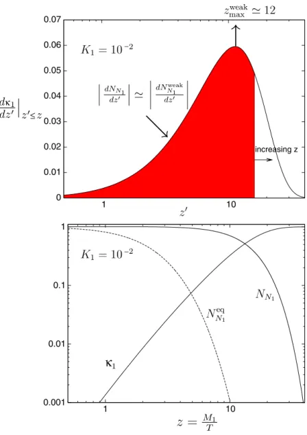
Figure 2. Dynamics in the weak wash-out regime for initial thermal abundance (N

1

= 1). Top panel: rates. Bottom panel: efficiency factor κ

and N

- abundance. The maximum of the asymmetry production rate occurs at z

z

= 1/ √

K

+ 15/8 12.

if ¯ z z

− 2. The value z

= z

(K

) is where the quantity ψ(z

, ∞ ) has a minimum and the integral in the equation (24) receives a dominant contribution from a restricted z

-interval centred around it. In the strong wash-out regime it is well reproduced by

z

(K

) 2 + 4 K

e

. (26)

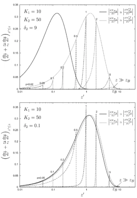
Figures 2 and 3 show, for an initial thermal abundance, the dynamics of the asymmetry generation, comparing one example of weak wash-out with one example of strong wash- out

. In the top panels we show the function dκ

/dz

≡ e

, defined for z

≤ z,

5 Corresponding animations can be found athttp://wwwth.mppmu.mpg.de/members/dibari.

JCAP06(2006)023

0.1 1 10

0.1 1 10

κ

κ

≤

0 0.05 0.1 0.15 0.2 0.25 0.3 0.35

0.001 0.01 0.1 1

>>

Figure 3. Dynamics in the strong wash-out regime. Top panel: rates. Bottom panel: efficiency factor κ

and N

-abundance. The maximum of the final asymmetry production rate occurs at z

z

.

for different values of z. The difference between the two cases is striking. In the weak wash-out regime, each decay contributes to the final asymmetry for any value of z

when the asymmetry is produced. In the strong wash-out regime, all asymmetry produced at z

z

− 2 is efficiently washed out by inverse decays, such that only decays occurring at z

∼ z

give a contribution to the final asymmetry.

The general expression equation (16) for ε

can be re-cast through the Ω matrix as [8]

ε

= ξ(x

) ε

(m

, M

, Ω

, Ω

) + [ξ(x

) − ξ(x

)] ∆ε

(m

, M

, Ω

, Ω

, Ω

). (27)

In the HL, for x

, x

1, one has ξ(x

) ξ(x

) 1 and then, from equation (27),

ε

= ε

(m

, M

, Ω

, Ω

). Therefore, in the HL the dependence on four of the see-saw

JCAP06(2006)023

parameters, namely M

, M

, Ω

, cancels out and one is left only with six parameters.

Notice moreover that κ

= κ

(m

, M

, K

), where K

= K

(m

, Ω

, Ω

), and thus the final asymmetry depends on the same six parameters too.

The HL for ε

can be written as [6] ε

(m

, M

, Ω

, Ω

) ≡ ε(M

) β(m

, Ω

, Ω

), where, writing Ω

≡ X

− i Y

≡ ρ

e

, with ρ

≡ | Ω

| ≥ 0, one has

ε(M

) ≡ 3 16 π

M

m

v

and β(m

, Ω

, Ω

) ≡

j

m

Y

m

j

m

ρ

. (28)

It is interesting that β(m

, Ω

, Ω

) ≤ 1, so that in the HL one has the upper bound

| ε

| ≤ ε(M

) [5, 6]. More precisely one can define an effective phase δ

by

β(m

, Ω

, Ω

) = β

(m

, m

) sin δ

(m

, Ω

, Ω

), (29) such that the upper bound [6, 13]

β

(m

, m

) = m

m

+ m

f (m

, m

) ≤ 1, (30) corresponds to sin δ

= 1 and it is obtained by maximizing over the Ω-parameters for fixed m

. The function f(m

, m

) is [8]

f(m

, m

) = m

+ m

m

Y

(m

, m

), (31) where Y

(m

, m

) is the maximum of Y

for Ω

= 0. For hierarchical light neutrinos, m

0.2 m

, an approximate explicit expression is [13]

f(m

, m

) = m

− m

1 + (m

− m

)/ m

m

− m

, (32)

which further simplifies to f (m

, m

) = 1 − m

/ m

for m

0.1 m

. Conversely, in the quasi-degenerate limit, one has f (m

, m

) =

1 − (m

/ m

)

[16]. One can then conclude that the maximum of the CP asymmetry is reached in the limit m

→ 0, when f (m

, m

) = 1 and, since this is true also for κ

, it also applies to the final asymmetry N

ε

κ

. For Ω

= 0 and Y

= Y

(m

, m

) the phase is maximal, while for a generic choice of Ω the CP asymmetry undergoes a phase suppression

sin δ

(m

, Ω

, Ω

) = m

+ m

m

f(m

, m

) (Y

+ σ

Y

) = (Y

+ σ

Y

)

Y

(m

, m

) , (33) where σ ≡

m

− m

/m

. One can see that sin δ

= 1 for Y

= 0 and Y

= Y

. It is instructive to calculate sin δ

for each of the three elementary complex rotations that can be used to parametrize Ω (cf (20)):

• For Ω = R

, one has sin δ

= Y

/Y

and the phase is maximal if Y

= Y

=

m

/m

; notice that there is no difference between normal and inverted hierarchy.

6 In [8] a minus sign in the expression forβ(m1,Ω21,Ω31) is missing. This does not affect any of the results but the quantitiesYi1 should be defined asYi1≡ −Im(Ω²j1) as here.

JCAP06(2006)023

10^-1 10⁰ 10¹ 10² 10³

10^-1 10⁰ 10¹ 10² 10³

10⁸ 10⁹ 10¹⁰ 10¹¹ 10¹² 10¹³ 10¹⁴

10⁸ 10⁹ 10¹⁰ 10¹¹ 10¹² 10¹³ 10¹⁴

invertedhierarchy

5x10⁹

K_atm K_sol

Nⁱⁿ_N

1

=1

5

M

1

T

in

K₁ 5

Nⁱⁿ_N

1

=0

2x10⁹

normalhierarchy

GeV

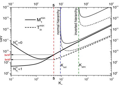
Figure 4. Lower bounds on M

and T

versus K

(cf (36) and (38)). Thick lines:

case of maximal phase (sin δ

= 1). Thin lines: case of very heavy N

.

• For Ω = R

, one has sin δ

= σ

Y

/Y

≤ σ, larger for inverted hierarchy compared to the normal one; however since κ

∝ K

[10] and since K

= K

| Ω

| for normal hierarchy and K

K

| Ω

| for inverted hierarchy, the final asymmetry is slightly higher for normal hierarchy compared to the inverted one for fixed | Ω

| [8].

• For Ω = R

, one has sin δ

= ε

= 0; one can check that ε

= 0 applies independently of M

and M

and therefore not only in the HL. Notice that the conclusions in the previous two cases are still valid if one multiplies R

or R

with R

respectively, since it does not affect sin δ

.

Interesting constraints follow if one imposes that the asymmetry produced from leptogenesis explains the measured value from WMAP plus SLOAN combined determination [7, 27],

η

(m

, M

, Ω

, Ω

) = η

= (6.3 ± 0.3) × 10

. (34) If M

10

GeV (m

/

i

m

), then M

N

a

16 π v

3

η

m

κ(K

) β

(m

, K

) sin δ

(Ω

, Ω

)

(35)

(M

)

≡ 4.2 × 10

GeV

κ(K

) β

(m

, K

) sin δ

(Ω

, Ω

) (at 3 σ C.L.).

(36)

This expression is quite general and shows the effect of the phase suppression [8] and of

a higher absolute neutrino mass scale [10] in making the lower bound more restrictive. In

figure 4 we show M

(thick solid line) for fully hierarchical light neutrinos (m

= 0) and

JCAP06(2006)023

maximal phase (sin δ

= 1). For K

5 one obtains the lowest value independent of the initial conditions [8],

M

5 × 10

GeV. (37)

The lower bound on M

also translates into a lower bound on T

, T

≥ (T

)

(M

)

z

(K

) − 2 2 × 10

GeV (K

5). (38) A plot of this lower bound is shown in figure 4 (thick dashed line). The relation between M

and T

can be understood from the top panel of figure 3, showing that the final asymmetry is the result of the decays occurring just around z

, when inverse decays switch off, whereas all asymmetry produced before is efficiently washed out.

4. Beyond the N

DS

There are three ways to go beyond the N

DS. We assume fully hierarchical light neutrinos.

4.1. N

DS

For Ω = R

, a nice coincidence is realized: the CP asymmetry ε

= 0 while ε

can be maximal and, at the same time, the wash-out from the N

inverse decays vanishes for m

10

eV. In this way the final asymmetry can and has to be explained in terms of N

decays. A nice feature is that the lower bound on M

does not hold any more, being replaced by a lower bound on M

that, however, still implies a lower bound on T

[8]. If one switches on some small R

and R

complex rotations, then the lower bounds on M

and T

become necessarily more stringent. Therefore, there is a border beyond which this scenario is not viable and one is forced to go back to the usual N

DS for successful leptogenesis. Account of flavour effects contributes to enlarge the domain where the N

DS works, since the wash-out from the lightest RH neutrino is diminished [28].

Notice moreover that, as in the N

DS, the lower bounds are more stringent for inverted hierarchy than for normal hierarchy, since in the first case K

K

while in the second case K

≥ K

.

4.2. Beyond the HL

If the RH neutrino masses are sufficiently close then the B–L asymmetry and the wash- out from the two heavier RH neutrinos have also to be taken into account and the general expression (6) for N

has to be used; at the same time, the general expression (27) for ε

has also to be used. Here the first, typically dominant, term can be enhanced by a factor ξ(x

) [13] while the second term can be calculated using [8]

∆ε

≡ 3 16 π

Im[(h

h)

] (h

h)

√ 1 x

= ε(M

) Im [

h

m

Ω

Ω

]

m

m

. (39)

One can see that ∆ε

vanishes for Ω = R

. It also vanishes in another interesting

situation, the strong–strong wash-out scenario for very large M

, that will be discussed

in detail in the next section. In these two interesting cases, the enhancement ξ(x

) is