Unfolding of the atmospheric
neutrino flux spectrum with the new program TRUEE and IceCube
Dissertation
zur Erlangung des akademischen Grades eines
Doktors der Naturwissenschaften (Dr. rer. nat.)
vorgelegt von
Dipl.-Phys. Natalie Milke
Dortmund, Juli 2012
Introduction 1
1 Motivation within astroparticle physics 5
1.1 Charged cosmic ray particles . . . . 6
1.2 Neutrino astronomy . . . . 7
1.3 Atmospheric neutrinos . . . . 8
2 Unfolding of distributions 11 2.1 Theoretical description of the implemented unfolding algorithm . . . 11
2.2 General remarks on unfolding . . . 15
2.3 Unfolding software TRUEE . . . 16
2.3.1 From RUN to TRUEE . . . 16
2.3.2 Adopted function . . . 18
2.3.3 New functions . . . 20
2.3.4 Supplementary tests for unfolding with TRUEE . . . 24
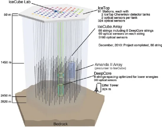
3 Determination of the atmospheric neutrino energy spectrum 29 3.1 The IceCube neutrino observatory . . . 29
3.1.1 Experimental setup . . . 29
3.1.2 Neutrino detection method . . . 32
3.1.3 Event reconstruction . . . 33
3.1.4 Simulation . . . 36
3.2 Neutrino sample . . . 39
3.2.1 Low level neutrino event selection . . . 39
3.2.2 High level neutrino event selection . . . 40
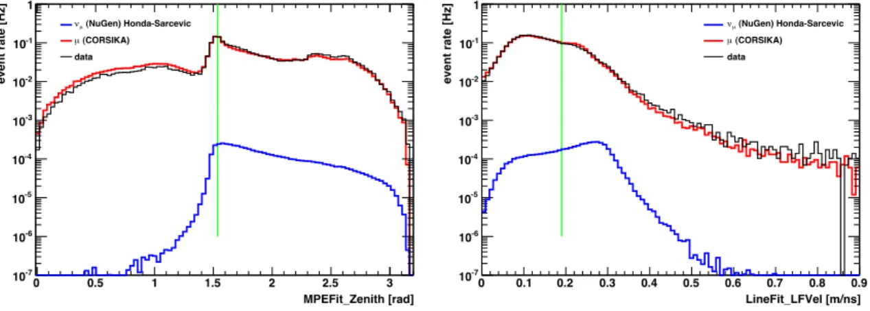
3.2.3 Data-simulation comparison . . . 46
3.3 Unfolding analysis with TRUEE . . . 50
3.3.1 Choice of energy-dependent observables . . . 50
3.3.2 Test mode results . . . 53
3.3.3 Pull mode results . . . 54
3.3.4 Unfolded atmospheric neutrino flux spectrum . . . 56
3.3.5 Verification of the result . . . 58
3.3.6 Zenith-dependent atmospheric neutrino spectrum . . . 60
3.4 Systematics studies . . . 61
3.4.1 Theoretical uncertainties . . . 61
3.4.2 Stability of the result against purity variation . . . 62
3.4.3 Depth-dependent unfolding . . . 64
3.4.4 Ice model comparison . . . 65
3.4.5 Final result with systematic uncertainties . . . 66
3.4.6 Depth-dependent correction of observables . . . 68
4 Summary and outlook 73 A Analysis development using 10 % of data 77 A.1 Tests on the observed zenith anomaly . . . 77
A.2 Background estimation with a new approach . . . 78
A.3 Depth-dependent tests of unfolding variables . . . 80
A.4 Resolution comparison of energy estimators . . . 81
A.5 General remarks . . . 82
Bibliography 83
Acknowledgment 90
High energy charged cosmic rays of unidentified origin arrive constantly at the Earth’s atmosphere. This particles reach energies up to 10 20 eV and are assumed to be accelerated by extragalactic sources. To track back the origin of cosmic rays the extragalactic high energy neutrinos have to be detected on Earth as their simulta- neous production is predicted by theories.
The neutrinos produced in the Earth’s atmosphere represent the main background for extragalactic neutrinos but at high energies their flux is expected to give way to the extragalactic flux. Therefore, the determination of the atmospheric neutrino flux spectrum can shed light on the contribution of extragalactic neutrinos to the measured flux spectrum.
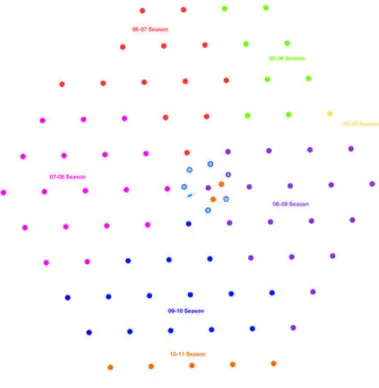
IceCube is a cubic kilometer large neutrino telescope located at the geographic South Pole and is well suited for the detection of high energy neutrinos. The data used for this work was taken while the experiment was under construction and thus the measurement proceeded with the partially finished detector IceCube 59.
For the determination of the neutrino energy a sophisticated algorithm is needed to estimate the energy distribution from the measured observables. For this purpose, TRUEE, the new unfolding program is developed based on the proven unfolding program RUN (Blobel, 1984). The software provides a large set of extensions to enable a comfortable and user-friendly unfolding analysis.
In this work the new software TRUEE is introduced and applied on the IceCube 59 data to estimate the flux spectrum of the atmospheric neutrinos. The software provides reliable results and the energy range of the spectrum could be extended.
The systematic uncertainties of the simulation have a large impact and have to be
reduced to make conclusions about the neutrino flux origin.
The evolution and structure of the universe and the natural laws of its internal en- tities have always attracted the mankind’s interest. That promoted the development of the research fields of particle physics, astronomy and cosmology. While particle physics studies the nature at very small scales by investigating particle interactions, astronomy and cosmology deal with large scales and describe properties of celestial objects and evolution of the universe as a whole.
In the recent decades these disciplines could find a common ground in the astropar- ticle physics, which studies the particles coming from the galactic and extragalactic sources. The latter can be studied from the characteristics of different particle fluxes. Of special interest are the high energy astroparticles (E > 10 11 eV), which are assumed to be accelerated by very distant and giant sources. The structure and mechanisms of such high energy accelerators can be studied as well as the medium the particles travel through.
Significant contribution to the latest interesting results could be achieved by pho- ton observations. Photons propagate without being deflected by magnetic fields and their spectra reveal the chemical and physical properties of the source. Giant extra- galactic sources, such as Active Galactic Nuclei, have been identified as one kind of accelerators for γ-rays with energies E > 10 13 eV.
A more challenging task is to track the origin of the charged cosmic ray particles, which are mostly protons, electrons and heavier atomic nuclei. A large spectrum of cosmic ray particles has been measured on Earth and reaches very high energies, E > 10 20 eV. Due to the galactic magnetic fields the charged particles are deflected and their arrival directions are randomized. Only for the very high energy cosmic ray particles the deflections are expected to be negligible. However, such particles have not yet been measured with sufficient statistics.
Theories about the acceleration of the charged cosmic rays predict an accompa- nying neutrino flux. Neutrinos interact only weakly with a very small cross section.
Therefore, they can escape from the source undistorted and travel long distances without being deflected. Thus, neutrinos are optimal candidates to find the accel- eration sources of charged cosmic rays. The high energy neutrino astronomy is a very young branch of the astroparticle physics and a high amount of discoveries is expected in the coming decades. Not only the origin of charged cosmic rays but also the evidence of magnetic monopoles, topological defects and dark matter particles are subjects for studies with the new neutrino telescopes [Hel11].
In the neutrino spectrum, which has been explored until today, the measurement
is dominated by the neutrinos coming from the cosmic ray showers induced in the
atmosphere. These atmospheric neutrinos represent the background for extraterres-
trial neutrinos. Therefore, the knowledge of the atmospheric neutrino flux spectrum is an essential part of the neutrino astronomy. The energy distribution of the at- mospheric neutrinos has a steeper slope than that of the predicted extragalactic neutrinos, coming e.g. from Active Galactic Nuclei. Hence, at very high energies the overall neutrino spectrum is assumed to be dominated by extragalactic flux with a corresponding flattening of the distribution. For this reason, the energy spectrum of all neutrinos arriving at Earth at very high energies provides information on a possible contribution of extragalactic neutrinos.
Due to the small cross sections the detection of neutrinos requires a large detector volume and a long observation time. In this way neutrino measurements can be col- lected with large statistics. The world’s largest neutrino telescope, IceCube [A + 11c], has been completed at the end of 2011 and is now in operation with its fully in- strumented detector volume of one cubic kilometer, located in the glacial ice at the South Pole. The neutrinos are identified by the measurement of secondary particles, e.g. muons, that are produced by the weak interactions of neutrinos with matter and in turn emit photons, while traveling faster than the light in the detection medium.
Generally, ground-based astroparticle detectors suffer from finite resolution and limited, energy-dependent acceptance. Furthermore, the direct detection of as- troparticles and their properties is often not possible. Instead, the secondary par- ticles are detected and, from their measurement, the estimation of the primary energy has to be made. This is a so-called inverse problem. In reality, inverse prob- lems usually feature unfavorable properties and have to be resolved with numerical approximations. Due to the finite resolution an observed variable cannot unambigu- ously be attributed to a primary particle energy. The limited acceptance implicates an incomplete measurement. Moreover, the production probability and the prop- agation of secondary particles have to be considered as well. To obtain the best possible estimation of primary particle energy an unfolding method has to be used.
Unfolding is a technique to estimate the distribution of a variable that is not directly accessible by the detection method. It takes into account all imperfections of the measurement procedure and can provide a result with a precision that is compatible with the detector configuration and statistical accuracy. Consequently, a sophisti- cated and feasible unfolding software is an essential instrument in the astroparticle physics analyses.
The general software development has made large progress during the last decades by using increasingly flexible programming languages. In many research fields the object-oriented C++ programming language is widely used in many applications.
Especially in the particle physics the C++-based ROOT [BR97] framework con- tains a high number of numerical methods and supplies advanced graphical tools.
The goal is to provide a new unfolding software that is user friendly, easy to in- stall and simply extendable. Considering these conditions a new unfolding software TRUEE [M + 12] has been developed by using C++ and graphical tools of ROOT.
The internal unfolding algorithm of TRUEE is based on the well tested RUN soft-
ware [Blo84] that was developed in FORTRAN 77 thirty years ago. RUN has been
proven to provide reliable results and realistic error estimation. Its ability to esti-
mate steeply falling distributions makes the algorithm optimal for the application in astroparticle physics.
The development of TRUEE and its application in the atmospheric neutrino ana-
lysis with IceCube is the objective of the present thesis. Since the IceCube telescope
was build over several years, the measurement has been performed with the partially
constructed detector. In the first chapter a general motivation on the atmospheric
neutrino analysis is given. The second chapter is focused on the inverse problems
and their solution with the TRUEE unfolding software. The advantages of the main
algorithm are pointed out and the newly implemented software features are intro-
duced. Chapter 3 covers the experimental part of the thesis. It starts with the
explanation of the detection method, followed by the event reconstruction and the
simulation, and proceeds with the individual steps of the analysis. Elaborated event
selection techniques, which have been developed in Dortmund as well, are applied
in the present analysis to deal with the very high background contamination of the
measurement. The application of TRUEE on the data is described and the system-
atic uncertainties are estimated. The conclusions of the whole work and the outlook
can be found in the last chapter. The technical details of the analysis development
are left to the appendix.
The main incitation of the current thesis is the contribution to the understanding the origin of the charged high energy astroparticles. It is well known, that giant cosmic particle accelerators, such as Active Galactic Nuclei (AGN) produce high energy γ-rays, which have been detected and studied by several experiments, see e.g.
Ref. [A + 07a], [FS09], [Pun05]. In contrast, the origin of charged high energy cosmic particles could not be identified, yet. The deflection of particles with energies up to E < Z · 10 17 eV by magnetic fields randomizes their arrival directions. Furthermore a suppression of the flux of proton dominated cosmic rays at high energies has been predicted, known as is the Greisen-Zatsepin-Kuzmin (GZK) cutoff [Gre66], [ZK66].
The protons with energies above E > 6 · 10 19 eV interact with the cosmic microwave background and thus loose their energy.
To shed light on the origin of charged cosmic rays and ensure the measurement at higher energies, we need particles which are connected to the charged cosmic ray production and can pass long distances without loosing directional or energetic information. Neutrinos are such particles and neutrino astronomy is the new growing branch of astroparticle physics. An identification of high energy neutrinos from extragalactic sources could be the missing link between the γ-rays and charged cosmic ray particles as the origin would be considered as the same for both kinds.
The bigger part of neutrinos measurable with the modern high energy neutrino telescopes are atmospheric neutrinos. These are produced in the extensive air show- ers caused by interactions of cosmic rays with the atomic nuclei of the Earth’s atmosphere. The atmospheric neutrinos represent major background for the ex- traterrestrial neutrinos. However, their dominance is decreasing at high energies due to the steeply falling energy spectrum. At very high energies a flattening of the spectrum is expected due to the contribution of flatter extragalactic spectrum.
Therefore, the study of the full neutrino spectrum measurable on Earth is performed
to confirm or reject the predicted flux model of extragalactic neutrinos. Additionally,
conclusions about the cross sections of charmed meson production due to interaction
of cosmic rays with the atmosphere can be made, as the related secondary neutrinos
have a slightly flatter spectrum as well.
1.1 Charged cosmic ray particles
The charged cosmic rays are composed of electrons, protons and atomic nuclei with different compositions depending on the energy, as explained below. The particles arrive the Earth’s atmosphere with energies up to 10 20 eV as has been observed already in 1963 by the MIT Volcano ranch array [Lin63]. In Fig. 1.1 the cosmic ray energy spectrum is shown measured by different experiments. The observed differential cosmic ray flux is dN dE ∝ E −γ , where the spectral index γ varies between 2.7 and 3.2 depending on the energy region. The features in the spectrum have to be noticed where the spectral index changes, because they indicate a change of the cosmic ray origin. Up to energies E ≈ 3 · 10 15 eV (the knee) the particles are expected to have galactic origin, e.g. from super nova remnants. At the knee the galactic contribution to the cosmic rays is assumed to decrease due to the Hillas condition [Hil84]
E max = β · Z · B · R, (1.1)
which restricts the maximum acceleration energy E max of a particle with charge Z by the relation between the magnetic field B and the radius R of the accelerating object. β is the characteristic velocity of the accelerating regions in terms of speed of light. Hence, the maximum acceleration energy of the primary cosmic ray particles from same sources is raising with the increasing particle charge. Therefore the flux from the galactic contributions does not drop down instantly at the knee but has a smooth decreasing distribution with a primary particle composition shifting toward heavier primaries at higher energies. This has been confirmed by the measurements of the composition of cosmic rays in the knee region [S + 02], [A + 05].
At the energies around E ≈ 3 · 10 18 eV the next feature, the ankle with subsequent flattening of the spectrum is observed. Here the contribution of the extragalactic sources is assumed to dominate. The galactic sources cannot produce such high energetic particles, which would escape from the galaxy at lower energies anyway, due to the large gyro-radius. The measurement of the primary composition around the ankle reveals a change from a steeper heavy nuclei spectrum to a flat proton- dominated one towards higher energies [B + 93]. Considering Eq. 1.1 this is a strong indication for a transition from galactic to giant and powerful extragalactic sources for charged cosmic ray particles.
As predicted, the spectrum drops very abruptly at energies above E ≈ 4 · 10 19 eV.
The trend to a flux suppression at high energies has already been visible in the
Yakutsk observation [K + 85]. The statistically significant measurement was pro-
vided by HiRes [A + 08a] and confirmed by the results of the Pierre Auger Observa-
tory [A + 08b]. Further measurements are needed to clarify whether the suppression
is caused by the predicted GZK cutoff or is due to the maximum acceleration energy
of the most source. This problem can be solved by the measurement of ultra high
energy cosmogenic neutrinos that are produced in the decay of mesons from the
proton-γ interactions [BZ69].
log10(E p /GeV) E p 2 ·dN p /dE p [ GeV cm -2 s -1 sr -1 ]
10 -9 10 -8 10 -7 10 -6 10 -5 10 -4 10 -3 10 -2 10 -1
1
2 3 4 5 6 7 8 9 10 11 12
Fig. 2. All particle Cosmic Ray spectrum. Data points come from the experiments as listed in the bottom left corner: Auger [YA + 07], HiRes [Hig02], AGASA [Y + 95a], KASCADE [A + 05, HK + 03]. Yakutsk [K + 85], Haverah Park [A + 01], HEGRA [A + 99], CASA-MIA [G + 99], Akeno [K + 85], Tibet [OT + 03], Tien Shan [A + 95a], MSU [K + 94], JACEE [A + 95b], Proton-Sat [G + 75].
(a) magnetic deflection is considered to a certain amount (ψ is larger than the point spread function of the detector),
(b) only the local Universe is considered (the choice of z max leaves out distant galaxies),
(c) only events with the highest energies are considered. Events of energies below E th are discarded, since lower-energy events are more sensitive to magnetic field deflections.
11
Figure 1.1: Differential flux of charged cosmic ray particles arriving on Earth and measured by different experiments. The flux is weighted by the square of energy to visualize the characteristic features. The structure around E ≈ 3 · 10 15 eV is called the knee. The particles with energies up to the knee have galactic origin and the spectral index is γ = 2.7. Above the knee the spectrum becomes steeper with γ = 3.2, where the contribution from the galactic sources such as supernova remnants is declining. The feature around E ≈ 3 · 10 18 eV is known as the ankle and signifies the probable transition from galactic to extragalactic sources for cosmic rays.
Picture is taken from Ref. [Bec08] where full references to the results can be found.
1.2 Neutrino astronomy
The possible extragalactic sources for charged high energy cosmic rays are AGN
and Gamma Ray Bursts (GRB). Assuming charged π-production in these sources
by hadronic interactions during the acceleration process, the component of high energetic neutrinos in the extragalactic cosmic rays is expected. Coming straight from the source without any deflection and interacting only weakly, extragalactic neutrinos are ideal candidates to perform a deep study of the accelerating objects.
The most favored model to describe the mechanism for particle acceleration in a galactic cosmic ray source is the first order Fermi acceleration [Fer49]. It suggests the acceleration of the charged particles due to magnetic deflection within propagating gas clouds with the additional influence of a shock region. The energy spectrum of the first order Fermi accelerated primary particles is expected to follow the flux dN dE ∝ E − 2 . Due to the high density of matter and radiation around the accelerating object the charged particles undergo further interaction. Only neutrinos from charged π- decays produced in particle collisions retain the primary flux distribution. Therefore the search for extragalactic charged particle accelerators can be restricted to the search of neutrinos with the spectral index γ = 2.
1.3 Atmospheric neutrinos
The main component of the atmospheric neutrinos is represented by the conven- tional neutrinos, coming from the cosmic ray induced productions of the charged K and π mesons, due to interactions with atomic nuclei N in the atmosphere
p + N → π + + π − + K + + K − + ... (1.2) and their subsequent decay into leptons
π + (K + ) → µ + + ν µ (1.3)
π − (K − ) → µ − + ν µ . (1.4)
The neutrinos from the following µ-decay can be neglected in the current analysis because the atmospheric muons above a GeV begin to reach the ground. For the same reason the flux of conventional atmospheric electron neutrinos is suppressed to higher energies [Gai07]. In the following only the muon neutrinos (and antineutrinos) are considered.
Due to the relatively long lifetimes of few 10 −8 s the K and π mesons undergo interactions in the atmosphere and thus, lose a part of their energy before decay.
On account of this energy loss the resulting atmospheric neutrino flux has a spec- tral index γ ≈ 3.7 and has therefore a steeper distribution, than the primary flux.
Moreover, the conventional neutrino flux distribution depends on the zenith angle.
Mesons, which travel through the atmosphere vertically, experience a larger density gradient, than the horizontally traveling mesons. Therefore, the interaction proba- bility of vertically incoming mesons is high and leads to the energy loss and hence, decreasing of measured flux.
For higher astroparticle energies (> 100 TeV) the production of mesons (D ± , D 0 ,
D 0 , D s ± , Λ + c ) containing charm quarks is possible [Gai03]. These massive and ex-
tremely short living mesons with lifetime shorter than 10 −12 s decay promptly after
production without interacting with the atmosphere, as shown here exemplarily for two decay channels of D-Mesons:
D 0 → K − + µ + + ν µ (1.5)
D + → K − + π + + µ + + ν µ . (1.6)
Hence the energy distribution of the original cosmic rays is conserved in the resulting neutrino spectrum and no zenith dependency of the flux is assumed. Therefore, this so-called prompt neutrino flux follows the power law with the spectral index γ ≈ 2.7.
Due to the similar branching ratios the prompt electron and muon neutrino fluxes are expected to be roughly the same [B + 89], [ERS08].
/GeV) (E ν
log 10
2 2.5 3 3.5 4 4.5 5 5.5 6 6.5 7
] -1 sr -1 s -2 [GeV cm ν Φ ν 2 E
10 -11
10 -10
10 -9
10 -8
10 -7
10 -6
10 -5
10 -4
10 -3
RECENT RESULTS (IC 40)
-2
90 % upper limit astrophys. E
νν
µunfolding
CONVENTIONAL Honda (Honda et al.) Bartol (Barr et al.)
PROMPT
Sarcevic (Enberg et al.) Naumov RQPM (Bugaev et al.)
Figure 1.2: Atmospheric muon neutrino flux spectrum averaged over the Northern hemisphere and weighted by the square of neutrino energy. Shown are the theoretical models for the conventional flux of Honda [H + 07] and Bartol [B + 04]. Additionally the models of Sarcevic [ERS08]) and Nau- mov [B + 89] for the expected prompt flux from charm meson decays are displayed. The most recent results from IC 40 analyses show the upper limit for the astrophysical E −2 flux [A + 11a] and the atmospheric flux estimation from the unfolding analysis [A + 11d].
Figure 1.2 shows the different theoretical predictions for conventional and prompt
atmospheric muon neutrino fluxes. The presented fluxes are averages over the zenith
region of the northern hemisphere, for a consistent demonstration throughout the
thesis. For the analysis the models of Honda et al. (in the following referred to
as Honda) and Enberg et al. (in the following referred to as Sarcevic) are used in
the simulation. Besides the theoretical predictions, the newest result of the atmo- spheric unfolding analysis and the search for isotropic astrophysical flux are given.
The results have been obtained with the data from the half complete IceCube de- tector of 40 string configuration (IC 40) and demonstrate that the experiment is approaching the energy region of high interest, where the contribution from prompt and astrophysical flux is expected to have an non-negligible impact.
Further predictions on the possible distribution of the atmospheric neutrino flux under consideration of the primary cosmic ray flux variations and the influence of the cosmic ray knee can be found in the Ref. [FBTD12]. In the same Reference the contribution of pion decays is assumed to be negligible for high energies, since the main contribution for conventional neutrinos can be charged to the kaon decays.
In general the conventional and prompt neutrinos as well as extraterrestrial neu- trinos are assumed to cause same signal pattern in the neutrino telescopes, thus an individual event cannot be classified as atmospheric or extraterrestrial, apart from the ultra high energy cascades, that are subject of other analyses [Joh11]. Therefore the atmospheric neutrinos represent the most significant background for the sought extragalactic signal.
A possibility to identify the extragalactic signal is to determine the whole incoming neutrino flux at high energies with a high precision. The expected spectral index of extragalactic neutrinos (γ = 2) is lower then the γ of the atmospheric neutrino flux. The flattening of the whole incoming neutrino flux at high energies would be an indication of the extragalactic component.
Thus the precise estimation of the neutrino energy flux for as high energies as
possible is desired and is the subject of the present thesis.
The estimation of the atmospheric neutrino energy spectrum is a so-called inverse problem. The neutrinos themselves cannot be detected directly and thus a straight measurement of their initial energy is impractical. Only when neutrinos undergo weak interactions, it is possible to track their secondary leptons. From the signals, these leptons cause in the detector, conclusions about the neutrino energies can be made. Due to uncertainties and smearing effects in a measurement the handle of such inverse problems is not trivial.
The primary neutrino flux is folded with the neutrino cross sections, the detector response and the lepton range. This statistical problem requires application of sophisticated unfolding algorithms to obtain optimal solutions.
2.1 Theoretical description of the implemented unfolding algorithm
The general problem statement of an unfolding analysis is the determination of the distribution f (x), while a direct measurement of x is not accessible. Instead, the measurement of y-values is made which are correlated with x. The goal is to obtain a best-possible estimation of the f(x)-distribution extracting information from the measured g(y)-distribution. This is an inverse problem. In a real measurement the transformation between x and y usually implies a limited acceptance and a finite resolution of the detector. Therefore a distinct allocation of a value x to a value y is not possible due to the smearing effect and loss of measurements (events). Thus, the migration probability between the measured values as well as the escape of events have to be taken into account.
In mathematics this relation between f (x) and g(y) is called folding or convolu- tion 1 and can be described by the Fredholm integral equation [Fre03]
g(y) = � d
c A(y, x)f (x)dx + b(y), (2.1)
where g(y) is the distribution of the measured observable y that can be multidi- mensional. The integral kernel A(y, x) is called response function and implicates all effects of a measurement imperfection. Usually this function is unknown and has to be determined by using Monte Carlo (MC) simulated sets of x and y values that comply theoretical models of the measurement process. c and d are the integral
1 The term convolution is used only if the kernel fulfills the condition A(y, x) = A(y − x)
limits of the range where x is defined (c ≤ x ≤ d). b(y) is the distribution of an optional background. The solving of the Eq. 2.1 is called unfolding or in the special case deconvolution.
A real measurement deals with discrete values and a parametrization of dis- tributions is required. In the here presented algorithm the distribution f(x) is parametrized by the superposition of the Basis-spline (B-spline) [dB01] functions p j (x) with the corresponding coefficients a j
f (x) = � m
j=1 a j p j (x). (2.2)
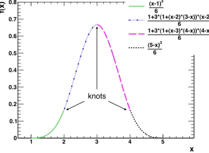
The B-spline functions consist of several polynomials of a low degree. In the following cubic B-splines are used, consisting of four polynomials of third degree (see Fig. 2.1).
The equidistant points where the adjacent polynomials overlap are called knots. The resulting parametrization provides function values at equidistant knot locations, but due to the smooth B-spline interpolation between the values a continuous function can be accessed. An afterward fragmentation of the function into a histogram with lower number of intervals helps to reduce the correlation between the data points.
An interpolation with B-spline functions does not tend to oscillations because of the low degree of the polynomials. With a given number of knots all B-spline functions
x
1 2 3 4 5
f(x)
0 0.1 0.2 0.3 0.4 0.5 0.6 0.7 0.8
6 (x-1) 3
6
1+3*(1+(x-2)*(3-x))*(x-2)
6
1+3*(1+(x-3)*(4-x))*(4-x)
6 (5-x) 3
knots
Figure 2.1: An example of a cubic B-spline function. The four polynomials of third degree overlap at the knots. Here the knot distances of 1 are chosen.
are defined and therefore only the coefficients a j have to be determined. Thus the B-splines can be included into the response function by integration over the whole x-region
� d
c A(y, x)f(x)dx = � m
j=1
a j
�� d
c A(y, x)p j (x)dx
�
= � m
j=1
a j A j (y). (2.3)
The piecewise integration over y-intervals A ij = � y i
y i − 1
A j (y)dy (2.4)
transforms the response function into a matrix with dimensions given by y-discretization (binning) and the number of knots. The same piecewise integration is made for the measured distribution g(y) and the background distribution b(y)
g i = � y i
y i−1 g(y)dy, b i = � y i
y i − 1 b(y)dy,
to obtain discrete histograms with content g i or b i in the interval (bin) i. The Fredholm integral equation 2.1 becomes a matrix equation
g = Aa + b. (2.5)
with vectors g, a and b and the response matrix A. To determine the sought distribution f (x) the coefficients a j need to be found.
The most straight forward method of solving the Eq. 2.5 is the inversion of the response matrix A, if the matrix is non-singular. Because of the measurement distortion, especially the finite resolution, the response matrix is not diagonal and the off-diagonal elements become more important if the resolution gets worse. This is the so-called ill-posed 2 problem. The ill-posedness can be revealed when the matrix is diagonalized. After arranging the eigenvalues in decreasing order a difference of several orders of magnitude between the highest and the lowest eigenvalue can be observed. Correspondingly, a large condition number indicates ill-posedness [WZ91].
The number is calculated as the ratio between the highest and the lowest singular values [Smi58], which are square roots of eigenvalues. An inversion of a matrix with such properties leads to increasing of the small off-diagonal elements which now gain strong influence on the result. Consequently a little variation in the values g i can cause large oscillations in the solution f (x). Therefore ill-posed integral equations generally cannot be solved by simple matrix inversion. To suppress the oscillations in the unfolded distribution, regularization methods are used. In the present algorithm a specific kind of the Tikhonov regularization is implemented [Tik63].
In its generalized form the Tikhonov regularization method suggests the linear combination of the unfolded fit with an operator multiplied by a regularization parameter τ . The operator implies some a-priori assumptions about the solution.
These can be e.g. the smoothness or monotony of the solution or the similarity of the unfolded function to a given trial function. Depending on the τ -value the
2 At least one of Hadamard’s conditions for a well-posed problem is not fulfilled. Those are the
existence of a solution, the uniqueness of the solution and the stability against slight changes
of initial conditions [Had02]
regularization term introduces a more or less bias into the solution towards an ex- pectation, and is therefore called penalty term. The same approach of regularization has also been invented independently by Phillips [Phi62]. The Phillips-method has been upgraded by Twomey [Two63] and hence has been extended to the treatment of overdetermined systems, which imply a non-square response matrix.
In the treated case a smooth result is expected and therefore the smoothness of the result has to be included as a mathematical constraint into unfolding procedure.
The smoothness is expressed by the curvature operator C. Due to the cubic B-spline parametrization of f (x), the curvature r(a) takes a simple form of a matrix equation
r(a) = � � d 2 f (x) dx 2
� 2
dx = a T Ca, (2.6)
with C as a known, symmetric, positive-semidefinite curvature matrix. During the unfolding as described in the following this curvature term will be included in the final unfolding fit equation (Eq. 2.10) and will be minimized considering the fit.
The unfolding as it is processed in the current algorithm does not involve the matrix inversion. After determining the response matrix A using MC simulated event sample, a maximum likelihood fit of the equation
g meas = ! Aa (2.7)
is performed that has the coefficients a i as free parameters. g meas is now the real measured observable distribution. To simplify matters a negative log-likelihood function S(a) is formed to be minimized:
S(a) = �
i
(g i (a) − g i,meas ln g i (a)). (2.8)
g i,meas is the number of measured events in an interval i including the possible background contribution in this region. The Poisson distribution in the bins is assumed with mean values g i . A Taylor expansion of the negative log-likelihood function can be written as
S(a) = S(˜a) + (a − ˜a) T h + 1
2 (a − ˜a) T H(a − ˜a), (2.9) with gradient h, Hessian matrix H and ˜a as a first assumption of coefficients, which is determined by an initial least square fit in the algorithm. The defined log-likelihood fit alone would lead to unrealistic fluctuating results for the mentioned reasons of an imperfect measurement, and therefore has to include the regularization term 2.6.
The final fit function
R(a) = S(˜a) + (a − ˜a) T h + 1
2 (a − ˜a) T H(a − ˜a) + 1
2 τ a T Ca (2.10)
has to be minimized to obtain the estimation of the B-spline coefficients. At the
same time a suitable value for the regularization parameter τ has to be found, to
get an optimal estimation of the result as a balance between oscillations and the smoothing effect of the regularization.
The here used method to define a value for τ implements the relation between τ and the effective number of degrees of freedom ndf
ndf = � m
j=1
1 1 + τ S jj
. (2.11)
S jj are the eigenvalues of the diagonalized curvature matrix C, arranged in increas- ing order. The summands in Eq. 2.11 can be considered as filter factors for the coefficients, which represent the measurement after internal matrix transformation.
They are arranged in decreasing order. Hence, the filter factors of higher index j suppress the influence of insignificant coefficients. Consequently a variation of τ reg- ulates the considered amount of information from the measurement and the number of degrees of freedom. In turn, the definition of number of degrees of freedom allows to specify the number of filter factors and thus the regularization strength.
To obtain Eq. 2.11, the Hesse and curvature matrices in Eq. 2.10 have to be diagonalized simultaneously. For this purpose a common transformation matrix can be found, that transforms the Hesse matrix into a unit matrix and diagonalizes the curvature matrix.
A lower limit of the parameter τ can be estimated by testing the statistical rele- vance of the eigenvalues of the response matrix. Applying Eq. 2.11, the number of degrees of freedom has to be chosen such that τ is above the suggested limit, in order to avoid the suppression of significant components in the solution. For more detailed information about the algorithm and mathematical descriptions see Ref. [BL98] and Ref. [Blo84]. Additionally to the unfolded result a full covariance matrix can be calculated following the error propagation. Therefore, a full information about the data point correlations can be obtained and used for testing theoretical models.
2.2 General remarks on unfolding
The solution of the inverse ill-posed problems is a challenging operation. The careful selection of observables and determination of binning of distributions and the regularization parameter is essential, to avoid a non-negligible bias of the result.
In cases, when only the comparison of the result with the existent theoretical pre- diction is needed, it is indeed simpler to fold the theoretical model and afterwards make the comparison with the measurement, and thus avoid unfolding itself [Lyo11].
Nevertheless unfolding is a mighty tool and is always needed when results of dif-
ferent experiments have to be compared or when the distribution parameters have
to be extracted after fitting the result by a function. Furthermore the storage of
the response matrix or the necessary MC simulation is dispensable if the unfolding
result is saved instead of the measured distributions. Thus, the comparisons with
theories developed in the future are not impeded by lack of the response matrix.
Since the introduced unfolding method accounts for event migration between data points and estimates the uncertainties correctly, it gives more reliable results than for example the simple and still widely used bin-by-bin correction factors method.
Also the dependence of the result on the MC assumption is in the latter very high.
A detailed discussion on different approaches for solving inverse problems can be found e.g. in Ref. [Blo10].
2.3 Unfolding software TRUEE
TRUEE (Time-dependent Regularized Unfolding for Economics and Engineering problems) [M + 12] is a software package for numerical solution of inverse problems (see Sec. 2). The basis for the algorithm is provided by the application RUN (Regularized UNfolding) [Blo84]. The algorithm-internal mathematical operations for the solution of the ill-posed inverse problems are described in Sec. 2.1.
2.3.1 From RUN to TRUEE
The unfolding program RUN was developed in the early 1980’s and was updated the last time in 1995 [Blo96]. Originally the algorithm has been developed and applied in the experiment CHARM, to determine the differential cross sections in the neutral current neutrino interactions [J + 81], [J + 83]. For the realization the programming language FORTRAN 77 was used. The graphical output is produced by making use of the Physics Analysis Workstation (PAW), an analysis tool of the FORTRAN 77 program library CERNLIB [CER93].
One of the main advantages of RUN is the event-wise input of all data. Accord- ingly the user can choose an individual binning for the response matrix. Furthermore additional cuts or weightings can be applied if necessary, without changing the data files. Moreover, based on event-wise input a verification of simulation and unfolding result could be developed (see Sec. 2.3.2). Up to three measured observables can be used for the unfolding at the same time and enhance the precision of the estimated function by extracting complementary information from the three observables. To achieve a physically meaningful result that is correct in shape and magnitude, an internal correction is performed by using the function of initially generated MC events. This function can be given by the user. Hence a correct reconstruction of the full distribution can be made even if the MC sample for the response matrix contains no events outside the measurement acceptance.
As described in the previous section the Tikhonov regularization is used assuming
a smooth distribution of the unfolded function. This is a proper assumption for the
astroparticle physics where in general the distributions do not show strong fluctu-
ations or very narrow peaks. Above all the prior usage of RUN in astroparticle
physics shows, that the algorithm is able to estimate a very steep distribution with
function values covering several orders of magnitude and therefore provides a perfect
basis for the here presented work [Goz08], [Cur08], [A + 10b].
The unfolding algorithm RUN has been tested and compared with different appli- cations. It stood out with notably stable results and reliable uncertainties [A + 07b].
Today it is still used especially in the high-energy physics experiments.
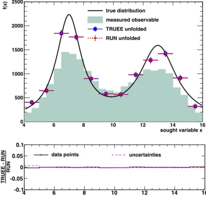
Nowadays the programming language C++ is widely used in several research fields. Primarily for this reason the unfolding software TRUEE has been developed, starting in 2008 and is now being maintained and frequently upgraded. The software contains the C++ converted RUN algorithm and additional extensions to make the unfolding procedure more comfortable for the user. Furthermore, the extension of the algorithm to a two-dimensional unfolding is intended, for studying of e.g. time- dependent variations of estimated distributions. The results of the new and original algorithms are identical as shown in Fig. 2.2 using MC simulated toy function f(x) of an arbitrary variable x.
sought variable x
4 6 8 10 12 14 16
f(x)
0 500 1000 1500 2000 2500
true distribution measured observable TRUEE unfolded RUN unfolded
4 6 8 10 12 14 16
RUN TRUEE - RUN
-0.1 -0.05 0 0.05 0.1
data points uncertainties
Figure 2.2: Comparison of the results of the original unfolding algorithm RUN (red/circles) and the new C++ version TRUEE (blue/squares). The solid black line is the true sought distribution. The shaded area repre- sents the measured observable that is used for the unfolding. The relative difference between bin contents and uncertainties from both algorithms can be seen in the lower figure and show a good agreement between the unfolding results.
The new software allows an easy installation of the software package by using the
build system CMake [MH03]. The comfortable creation of graphics benefits from
the high variety of graphical tools in ROOT [BR97]. The new additional functions
such as test mode (see Sec. 2.3.3), make the choice of unfolding parameters and observables easier for the user. The most important functions are introduced in the following sections, while the complete information about the new extensions and the handling of the software can be found in the TRUEE manual, that is provided along with the source code [Tru12].
2.3.2 Adopted function
The original unfolding software RUN offers already some helpful tools that give the user the opportunity to check the performance of the unfolding procedure. They have been adopted in the new unfolding software and therefore are briefly introduced in the following.
Verification of the result and simulation
This method is executed after the unfolding and can be used to test the agreement between data and simulation and to check the unfolding result. The distributions of simulated and measured observables do not necessarily match in shape since the true distribution is not known. Therefore the unfolded and the MC distributions of the sought variable are different. After the unfolding the MC events are weighted such that the MC distribution of sought variable describes the unfolded function. In this case also the measured and simulated observable distributions have to match. This procedure is comparable to the first iteration of the forward-folding method [M + 06].
For every observable a data and MC histogram value is produced and the corre- sponding χ 2 is calculated and can be viewed by the user. If one of the observables does not match, it is likely that this observable is not correctly simulated. If all observables show disagreement between data and MC then either the observables used for unfolding are not correctly simulated or there is a general data MC mis- match. To exclude the possibility of improper choice of unfolding parameters, prior unfolding tests on MC sample have to be carried out, as explained in Sec. 2.3.3.
Nevertheless, various unfolding results with slightly changing parameters should be made also with measured data to test the stability of the result. The χ 2 of the presented verification method can be used for this testing purpose.
Test of the covariance matrix
An accurate estimation of a distribution requires a low correlation between the
data points while the number of data points is as high as possible. This way the
result comprises all important characteristics of a distribution with minimized bias
and uncertainties. Because of the finite resolution of a measurement the final result
will always have correlated bins, especially if the bin width is much smaller than the
resolution. The negative correlations are dominant, if the regularization is low or
in the extreme case non existent at all. The result fluctuates wildly and has unrea-
sonably large uncertainties. With increasing regularization the positive correlations
become important and the characteristic features of distribution begin to vanish.
It is the users challenge to keep balance between the correlation extrema. There- fore the subroutine to monitor the data point correlation by testing the covariance matrix has been developed. The correlation between data points is considered as negligible if the covariance matrix of the result is roughly diagonal. Accordingly, the test assumes a diagonal covariance matrix and checks generated statistical devi- ations from the result as explained in the following. A random Gaussian deviation f ˜ (x i ) of the estimated bin content f (x i ) in every bin i is generated 5 000 times. For every deviation the value z is calculated:
z = � n
i=1
(f(x i ) − f(x ˜ i )) 2
σ i 2 , (2.12)
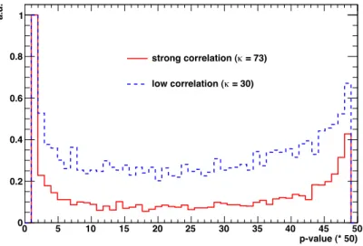
where σ i is the i’th diagonal element of the covariance matrix and n is the number of bins. The z 2 value is converted to a p-value which is then multiplied by 50. The resulting values are restricted to the range between 1 and 50 with interval width of 1, so that values outside this limits go into the outer bins. The distribution of the 5 000 p-values is visualized in a histogram. For statistically independent data points a flat uniform distribution of p-values is expected with mean bin content at 100. For a strongly correlated data points the p-value histogram shows a “sagging clothesline” behavior with very large outer bins (compare Fig. 2.3). Since there is always a slight correlation between the data points, the user has to decide when the distribution is flat enough and the covariance matrix can be assumed as diagonal. In
p-value (* 50)
0 5 10 15 20 25 30 35 40 45 50
a.u.
0 0.2 0.4 0.6 0.8 1
= 73) strong correlation ( κ
= 30) low correlation ( κ
Figure 2.3: Comparison of p-value distribution for strong correlation among the data point (red) and the much flatter distribution for lower correlations (blue).
The distributions maxima have been scaled to 1.
TRUEE the flatness is checked by calculating the deviation of the p-value histogram
bin contents from the value 100. The such constructed correlation value κ κ = � 50
i=1
(bin content i − 100) 2
50 (2.13)
has to be minimal. Independent tests using known unfolded distributions showed that the correlation value should be κ ≤ 50. This value range can be large, depending on the resolution and additional test is required as presented in Sec. 2.3.3. A further discussion on the data point correlation can be found in Ref. [Blo10].
2.3.3 New functions
The experience in working on inverse problems reveals, that some standard oper- ations have to be carried out as preparation for the actual unfolding. As examples can be listed the selection of the suitable unfolding observables, which provide the highest amount of information about the sought distribution, as well as the selection of the optimal settings for the unfolded function, such as binning of the response matrix or the regularization parameter. Considering these requirements, additional functions have been implemented in TRUEE to make the unfolding analysis more comfortable and user-friendly. In the following the most important functions are introduced using an exemplary toy MC distribution f (x).
Selection of Observables
The selection of suitable observables for the unfolding is crucial for estimating the result with high precision. An appropriate set of observables leads to result that is stable against moderate changing of regularization. The available event tuple file usually contains a large set of different observables. Since only three observables can be used for the unfolding fit at the same time, the user has to choose the best combination of maximum three observables to obtain a good estimation of the demanded distribution. The highest information content about the sought distribution is provided by observables, which have a strong correlation with the sought distribution. The correlation can be visualized in scatter plots with sought variable versus observable. Such scatter plots are created in TRUEE automatically for every input observable. Additionally the corresponding profile histograms are provided containing the mean value of the sought variable for every bin in the observable. A monotonically changing profile function over the whole range of the sought variable, together with small uncertainties, indicates a good correlation. The binning of the response matrix is equidistant, therefore a linear dependency between the observable and sought variable is optimal. In case of logarithmic dependency a transformed input of the observable or sought variable is possible.
The correlation between the chosen observables themselves should be as small as
possible to avoid redundancy.
0 100 200 300 400 500 600 700
y measured [a.u.]
2 4 6 8 10 12 14 16 18
x true [a.u.]
6 8 10 12 14
y measured [a.u.]
2 4 6 8 10 12 14 16 18
mean x true [a.u.]
4 6 8 10 12 14 16
Figure 2.4: Scatter plot (left) and profile histogram (right) of the toy MC. The profile histogram is obtained calculating the mean value of the ordinate within every abscissa bin of the scatter plot. A monotonic distribution of the profile with small uncertainties over the whole x region shows a good correlation between the distributions at the axes.
Preparatory unfolding tests in the test mode
It is a common strategy to check the unfolding performance on a set of MC simulated data before analyzing the real measured data. To facilitate this procedure the test mode has been developed. While running TRUEE in test mode only the MC simulated sample is analyzed. A user-defined fraction of events is selected from this sample and is used as pseudo data sample for unfolding. The remaining MC events are used in the usual way to determine the response matrix and scale the result. The unfolded distribution is compared to the true distribution using the Kolmogorov-Smirnov test [CLR67] and the χ 2 calculation. This method allows to restrict the space of the possible parameter regions and can be helpful in finding the optimal observable combination, if the definite choice could not be made by the observation of the profile plots (Fig. 2.4).
Selection of parameter sets
Generally, the user of an unfolding software has to define different parameters. In the most cases these are bin numbers for the observable and the unfolded distribution and the influence of the regularization. In TRUEE the user has the possibility to define ranges of parameters. The unfolding result is provided for all parameter combinations. The in Sec. 2.3.2 introduced κ is calculated for every result and can be compared among those. For this purpose a two-dimensional histogram is produced with the parameters number of degrees of freedom (ndf) and the number of knots (nknots) at the axes. Every histogram is produced for a fixed number bins and has the κ-value as bin content (see Fig. 2.5). This parameter selection tool can be used in the test mode as well as in the standard unfolding.
An upgrade of such parameter space histogram has been developed for the test
25 30 35 40 45 50 55 60
number of degrees of freedom
4 6 8 10 12 14
number of knots
10 15 20 25 30
Figure 2.5: Figure for selection of results with optimal unfolding parameter sets. The results are produced for different parameter settings and the resulting quality values are compared. The color-coded data point correlation value κ is compared for different results with varying ndf and nknots for a fixed binning of the result. The optimal results can be found in the region with low κ-value.
9 10 11 12
8 13
7 6 5 4
] 2
unfolded result
0 2 4 6 8 10 12
g data point correlation
30 35 40 45 50 55 60 65 70
Figure 2.6: Figure of an upgraded parameter selection technique. The unfolding
results are produced for different parameter settings and the resulting
quality values are compared. The figure shows the value κ versus the
χ 2 for different test mode results. Per default the results are numbered
successively for different sets of parameters. For presentation reasons
the results in this figure are labeled with ndf. The optimal results can
be found in the kink with low axes values (ndf = 8 − 10). The displayed
results include only the variation of ndf for simplicity.
mode. In the new histogram the κ-value is plotted versus the χ 2 -value from the comparison of the unfolded and true distributions. Each result is indicated by a successive numbers in accordance to the parameter loops in the code. A list with result indices and corresponding parameter settings is produced as well. The distribution of the results in the graphics is expected to follow a curve similar to the one of the L-curve method [HL74]. Hence the best results can be found in the kink of the curve with the lowest κ and the lowest χ 2 (compare Fig. 2.6).
The advantage of curve histogram is that it is not restricted to a fixed dimension of parameters but can be extended easily for further parameters. Moreover the unsuitable parameter sets can be easily identified and excluded very quickly due to the large result distance from the kink.
Statistical stability check with the pull mode
After the selection of parameter sets and the observables the performance of the final unfolding configuration should be tested with a high number of different toy MC samples. For this purpose the pull mode have been implemented in TRUEE.
Similar to the test mode only the MC sample is used and a pseudo data sample is chosen according to the expected measured data. The unfolding is executed with a fixed parameter set and the estimated and the true values are compared bin-wise.
The extracted information of the residuals is stored in histograms. This procedure should be executed several hundred times and allows to make conclusions about the stability of the unfolding against statistical variations as described in the following.
First the relative difference between true and unfolded f (x i ) value for every bin i is created as
true i − unf olded i
true i
. (2.14)
After few hundreds of pull mode runs the relative difference should follow gaussian distribution with the mean around zero. The deviation of the mean value from zero indicates a bias in this bin. The standard deviation of the distribution corresponds to the statistical uncertainty in the bin. Therefore the uncertainties of the unfolded function must not fall below this value.
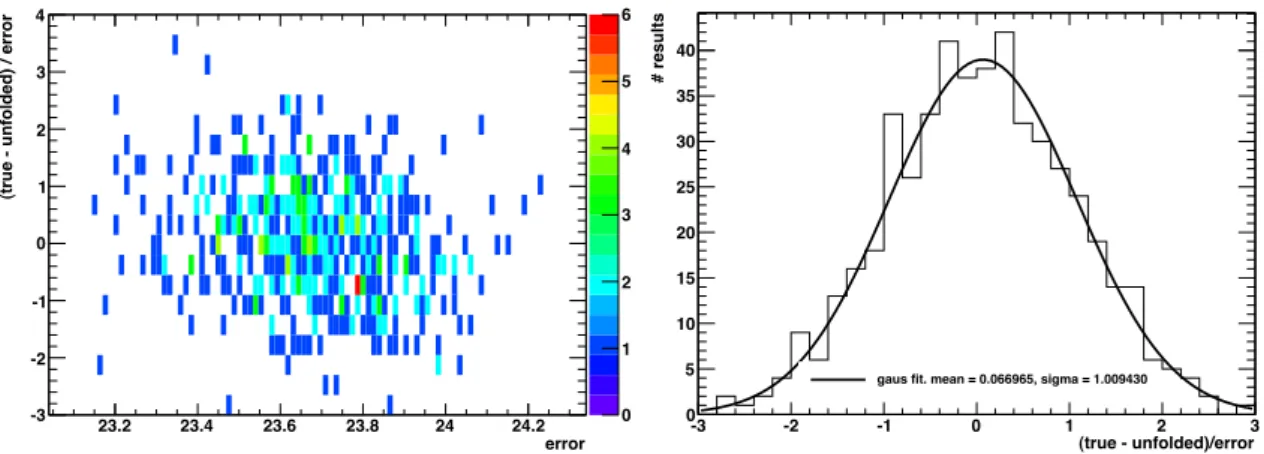
Furthermore, the so-called pull distributions in separate histograms for each bin i are created (Fig. 2.7). The abscissa indicates the estimated uncertainty obtained from the unfolding in this bin. On the ordinate the difference over the uncertainty
true i − unf olded i uncertainty i
(2.15)
is shown. After few hundreds of runs an optimal pull distribution appears as a
smooth cloud with the ordinate distribution between − 1 and +1 with mean value
at zero. A projection on the ordinate reveals a gaussian distribution. Any deviation
from zero indicate a bias in the considered bin. The clouds standard deviation σ
larger/smaller than the ± 1 interval means a general under-/overestimation of the
uncertainties in the bin.
0 1 2 3 4 5 6
error
23.2 23.4 23.6 23.8 24 24.2
(true - unfolded) / error
-3 -2 -1 0 1 2 3 4
(true - unfolded)/error
-3 -2 -1 0 1 2 3
# results
0 5 10 15 20 25 30 35 40
gaus fit. mean = 0.066965, sigma = 1.009430
![Fig. 2. All particle Cosmic Ray spectrum. Data points come from the experiments as listed in the bottom left corner: Auger [YA + 07], HiRes [Hig02], AGASA [Y + 95a], KASCADE [A + 05, HK + 03]](https://thumb-eu.123doks.com/thumbv2/1library_info/3648917.1503183/13.892.209.750.174.760/particle-cosmic-spectrum-points-experiments-listed-corner-kascade.webp)