Neutral non-equilibrium population genetics

Neutral non-equilibrium population genetics

Inaugural - Dissertation

zur

Erlangung des Doktorgrades

der Mathematisch-Naturwissenschaftlichen Fakultät der Universität zu Köln

vorgelegt von

Daniel Živković

aus Salzburg

Köln, 2008

Tag der letzten mündlichen Prüfung: 11. März 2009

Die Identifizierung genomischer Regionen, die von positiver darwinscher Selektion geprägt wurden, gilt als eines der zentralen Interessen der molekularen Evolutionsbiologie. Wenn eine Population ein neues Territorium besiedelt oder einer drastischen Umweltveränderung ausgesetzt ist, bedingt dies naturgemäß eine Schwankung in der Populationsgrösse. Den- noch beruhen die meisten statistischen Methoden, die adaptive Vorgänge in einer Popu- lation erfassen sollen, auf der Annahme einer konstanten Populationsgrösse. Erst in den letzten Jahren wurde Populationsgenetikern bewusst, dass Modelle variabler Populations- grösse für eine angemessene Interpretation von DNA-Polymorphismen unerlässlich sind.

Im Rahmen der Koaleszenztheorie werden theoretische Resultate für die zweiten Momente bestimmter Baummaße unter variabler Populationsgröße hergeleitet. Darüber hinaus werden Formeln für die zweiten Momente diverser DNA-Polymorphismus-Maße für allgemeine binäre Bäume entwickelt. Diese Resultate stellen das Herzstück der Dis- sertation dar. Mit Hilfe dieser Ergebnisse erhält man tiefere Einsichten in die Auswirkung variabler Populationsgrösse und grenzt das Problem der Unterscheidung adaptiver und demographischer Faktoren besser ein.

Im Folgenden werden verschiedene weit verbreitete statistische Testmethoden, die ursprünglich unter der Annahme einer konstanten Populationsgrösse konstruiert wur- den, verallgemeinert, sodass, wenn die demographische Entwicklung einer Population ausreichend bekannt ist, einzelne Loci gegen die Nullhypothese neutraler Evolution unter variabler Populationsgrösse getestet werden können. Dies wird anhand zweier X- chromosomaler Datensätze einer afrikanischen und einer europäischen Stichprobe von Drosophila melanogaster demonstriert.

Während das im Vorfeld vorgeschlagene Expansionsmodell für die afrikanische

Stichprobe erfolgreich in die verallgemeinerten Teststatistiken integriert werden kann,

bleibt eine adäquate Analyse für das Bottleneckmodell der europäischen Stichprobe

unerfüllt. Abschließend werden charakteristische Merkmale demographischer Modelle

vorgestellt, anhand welcher die Durchführbarkeit einer aussagekräftigen statistischen

Analyse nachvollzogen werden kann.

The identification of genomic regions that have been exposed to positive Darwinian selec- tion is of major interest in evolutionary biology. Although adaptive processes are generally associated with populations that experience an environmental change or colonize a new habitat, statistical tests were commonly constructed on the assumption of constant pop- ulation size. However, only in recent years did the practical need to account for models of variable population size become apparent in the attempts of population geneticists to properly interpret the rising amount of DNA polymorphism data.

Within the framework of coalescent theory, theoretical results regarding the second- order moments of certain tree size measures are derived under variable population size.

Thereafter, formulas for the second-order moments of diverse DNA polymorphism mea- sures are developed for general binary trees. These results constitute the centerpiece of this thesis. Their relevance lies in the possibility to obtain deeper insights into demographic factors and to better delimit the problem of distinguishing adaptive from demographic forces.

Several popular and widely applied statistical tests, that rest on the assumption of constant population size, are generalized, so that, conditional on knowledge of a demo- graphic scenario, single loci can be tested for traces of selection against the null hypothesis of neutral evolution under variable population size. This is demonstrated for two datasets of X-linked loci from an African and an European sample of Drosophila melanogaster .

While a previously suggested expansion model for the African sample can be suc-

cessfully implemented into the generalized test statistics, an adequate analysis for the

bottleneck model of the European sample cannot be accomplished. Consequently, we ex-

tract characteristic features of demographic models in order to distinguish the ones which

are accessible to a meaningful statistical analysis from those which are not.

1. Introduction 1

1.1 Theoretical population genetics 1

1.2 Modeling neutral and adaptive mutations 4

1.3 Testing the neutral mutation hypothesis 6

1.4 Organization of the thesis 8

2. General coalescent trees 11

2.1 Variable population size 12

2.1.1 Mean waiting times 13

2.1.2 Mean squared waiting times 20

2.1.3 Mean product of two distinct waiting times 25

2.1.4 Mean and variance of two tree size measures 31

2.2 Measures of DNA polymorphism 32

2.2.1 The number of segregating sites 32

2.2.2 Mutations of a certain size 33

2.2.3 The average number of pairwise differences 40

3. Testing neutrality under variable population size 41 3.1 The estimated demographic history of Drosophila melanogaster 41

3.2 Generalization of classical test statistics 45

3.2.1 Tajima’s D 45

3.2.2 Fu and Li’s D 50

3.2.3 Fay and Wu’s H 54

3.2.4 The singleton-exclusive version of Tajima’s D 57

4. Discussion 67

References 77

Introduction

1.1 Theoretical population genetics

Population geneticists are devoted to the analysis of the evolutionary forces that shape the patterns of genetic variation within species. These forces include mutation, recom- bination, natural selection, demographic processes and their interactions. Theoretical population genetics is the mathematical study of these evolutionary patterns and forces.

It is roughly divided into the development of conceptual models and theories (mostly based on the classical diffusion theory) and the advancements of statistical methods for data analysis (mostly based on coalescent theory).

Using the mathematical discipline of diffusion theory, classical population genetics is able to predict the impact of the evolutionary forces on allele or genotype frequencies at one or more loci of an entire population by looking forward in time. Once results for the whole population have been obtained, one can make predictions for a sample taken from the population, which is essential for the application of a chosen mathematical model to biological data. Initiated by the pioneering work of Fisher (1930b), Wright (1931) and Haldane (1932), diffusion models were state-of-art for decades, including important contributions by Malécot (1948), Feller (1951) and Kimura (1964). Sewall Wright introduced the concept of genetic drift—the random alteration in allele frequency of a population over time. Kimura (1968, 1983) established the neutral theory of molecular evolution. He argued that the vast majority of mutations are selectively neutral by having negligible effects on the reproductive ability of their carriers and that genetic drift is the primary evolutionary force—a hypothesis strongly opposed by Gillespie (1984, 2000).

Despite the development of some major principles of the neutral theory ( Kimura 1983),

the main advantage of the classical diffusion approach, in contrast to the coalescent-based

approach described below, may be seen in the modeling of natural selection, with par-

ticular regard to positive selection. Maynard Smith and Haigh (1974) introduced the

model of genetic hitchhiking, in which a selectively neutral allele or mutation may quickly spread through an entire population if it is linked to a beneficial mutation. Consequently, the increase in frequency of the selectively neutral mutation leads to a drastic reduction in its variability—a procedure commonly known as a ‘selective sweep’. Reformulating an ap- proach of Ohta and Kimura (1975), Stephan et al. (1992) obtained analytical results of the effect of a positive substitution on expected heterozygosity. However, addressing the same problem via coalescent theory is more cumbersome ( Kaplan et al. 1989).

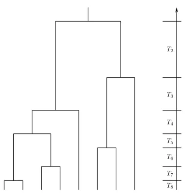
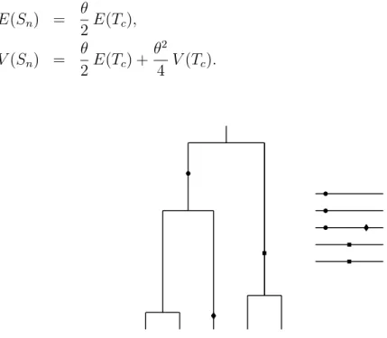
Based on the seminal papers by Kingman (1982a, b), coalescent theory has become the most popular branch of theoretical population genetics over the past 25 years. In contrast to the classical diffusion approach, a sample (rather than the entire population) of genes, or DNA sequences, is traced backwards in time up to the single ancestor of the entire sample, which is referred to as the most recent common ancestor (MRCA). Figure 1.1 illustrates this ancestral process in form of a bifurcating genealogy. The intuitive treatment of population genetical questions has propelled coalescent theory to a broader readership ( Hein et al. 2005, Wakeley 2008) due to the simpler acquisition of its basic principles, when compared to classical population genetics.

Another major advantage of this retrospective view of a sample in coalescent theory is given by the fact that computer simulations, which are often used to support mathe- matical approximations of specific models, are more time-efficient and easier to implement than classical, forward-in-time diffusion approaches.

T

T

T

T

T

T

T

Abbildung 1:

Figure 1.1 One possible coalescent tree of a sample of size eight. The waiting times until

a pair of genes end up in their common ancestor are denoted by T _i .

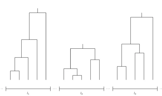
Rosenberg and Nordborg (2002) reapplied two substantial arguments regard- ing the relationship of the sample to a large, unstructured population and the im- portance of recombination as an evolutionary force. First, as it has been shown by Saunders et al. (1984), the probability that a sample of size n contains the MRCA of the entire population is simply (n − 1)/(n + 1). For this reason, even the genealogy for a small sample is likely to contain the MRCA of the population and encourages a focus on the sample rather than on the population as a whole. Furthermore, this means that increasing the sample size has a minor effect. Adding more sequences in Figure 1.1 would mainly change the lower part of the genealogical tree, whereas the lengths of the deep branches near the MRCA would be barely affected (cf. Hein et al. 2005). Second, the au- thors emphasized the importance of recombination for statistical inference. In the absence of recombination, there is only a single genealogical tree for an entire chromosome, such that a reliable prediction of its evolutionary history becomes arguable. In the presence of recombination, unlinked or loosely linked loci can be seen as independent replicates of the same ancestral process (cf. Figure 1.2). Therefore, variation sampled from a large number of preferably unlinked loci, which feature genealogies that are conditionally independent on the population’s demographic history, provide the necessary polymorphism data for population genetical inferences. In particular, this shall lead to an improvement of the estimates of a population’s demographic trend.

· · · · · · · · · · · ·

l

l

l

Figure 1.2 Possible coalescent trees for three different loci.

1.2 Modeling neutral and adaptive mutations

Mutations are the indispensable source of variation to develop an evolutionary under- standing of how demographic and selective forces have shaped present-day sampled DNA sequence variation data. Although these sequences reveal several types of ge- netic variation, such as copy number variations ( Redon et al. 2006) or microsatellites ( Tautz 1989), single nucleotide polymorphisms (SNPs) have become the prevalently analyzed form of polymorphism, especially from a theoretical standpoint. As such, only mutation models associated with SNPs are investigated throughout this thesis.

The two most prominent assumptions regarding mutations are the infinitely-many- sites model ( Kimura 1969, Watterson 1975) and the infinitely-many-alleles model ( Kimura and Crow 1964). Under the infinitely-many-sites model, each new mutation arises at a site in an infinitely-long DNA sequence where there has never been a mutation before. The infinitely-many-alleles model, assuming that each mutation generates a new allele, differs from the infinitely-many-sites model in the sense that one ignores how many mutations distinguish alleles and considers only whether alleles are the same or different. The fundamental accomplishment under the infinitely-many-alleles model is the discovery of the Ewens sampling formula ( Ewens 1972)—the probability distribution of a configuration of alleles in a sample of genes—under mutation-drift equilibrium.

Karlin and McGregor (1972) were the first to prove the Ewens sampling formula.

Griffiths and Lessard (2005) provided a proof by a direct combinatorial argument and extended the distribution to populations of varying size.

Watterson (1975) introduced the mutation parameter θ = 4Nµ, where N is the size of a diploid population—at time of sampling in the coalescent theoretical context and, in particular, under variable population size—and µ is the mutation rate per sequence per generation. The number of mutations of rate µ or θ/2, respectively, when time is measured in units of 2N generations, is typically Poisson-distributed in the sense that mutations are rare events. An important point in modeling selectively neutral mutations in the aforementioned manner is that these mutations have no impact on the structure of the genealogy of a sample. Consequently, the genealogical and mutational process can be separated; particularly when a population experiences changes in population size (see Chapter 2).

For the standard neutral model of constant population size, Watterson (1975)

devised the mean and the variance of the number of segregating sites, S n , which under

the infinitely-many-sites model equals the number of mutations that occur on the

genealogical tree. Later, Tavaré (1984) derived the probability distribution of S n .

Additionally, properties of other historically important test statistics, namely the average

number of pairwise differences, Π n , and the number of times a mutation can be observed

at specific sites of the sampled sequences, ξ i , have been derived within the coalescent

framework. Tajima (1983) calculated the mean and the variance of Π n and Fu (1995)

derived the means and the variances of ξ i of selectively neutral alleles within a given

sample under constant population size. Curiously, Fisher (1930a) already hinted at the

result for the mean of ξ i in the diffusion setting. The above results have been mostly

obtained without taking recombination into account. The derivation of theoretical results

that incorporates recombination is more complex, even for the standard neutral model, as can be seen in Kaplan and Hudson (1985), who established an approximation of the variance of S n , or Wakeley (1997), who derived the variance of Π n .

The study of temporal variation in population size has generated much interest since an early article by Wright (1938). Nei et al. (1975) have analyzed the effect of arbitrary population size changes on the average heterozygosity of a neutral locus.

Maruyama and Fuerst (1984) developed a numerical method for the mean number and average age of alleles in a population undergoing an instantaneous expansion.

Watterson (1984) derived analytical formulas, including the probability distribution and moments of the total number of alleles in a sample, for models of one or two sudden changes in population size. Tajima (1989a) derived the expected number of segregating sites and the expectation of the average number of pairwise differences for an instan- taneous population growth model. Slatkin and Hudson (1991) examined a model of exponential growth before Griffiths and Tavaré (1994) unified arbitrary changes in population size into a general framework. Moreover, Griffiths and Tavaré (1998) developed the frequency spectrum of neutral alleles in a population of arbitrary varying population size.

Besides fluctuation in population size, the study of population structure has become another population genetical subfield of a long-standing interest ever since its initiation by Wright’s island model ( Wright 1931), where a population is subdi- vided into discrete subpopulations with limited migration among them. Exemplarily, Takahata and Nei (1985) derived the variance of Π n in a two-population model without migration and Wakeley (1996) obtained the concordant result with migration.

Wakeley (2008) provides a comprehensive overview on population structure, which is not further investigated in this thesis.

Since the different types of natural selection influence the reproductive success

of the population’s individuals, advantageous or deleterious mutations—in contrast

to neutral mutations—have an effect on the genealogical tree. In addition to above

work on positive directional selection, several advancements under the assumption

of constant population size have been made. Wiehe and Stephan (1993) examined

questions concerning the strength and the frequency of selective substitutions in the

face of observable sequence data. Braverman et al. (1995) investigated the effect of

genetic hitchhiking on the site-frequency spectrum by using a computer simulation based

approach. Fay and Wu (2000) pointed out that an excess of high-frequency derived

variants is an unique characteristic of genetic hitchhiking. Gillespie (2000) introduced

the pseudohitchhiking model—a simplification of the typically studied two-locus dynam-

ics to a single locus—and argued that the recurrence of selected substitutions resembles

the stochastic behavior of genetic drift. Whereas the above articles have been built on

the initial suggestion by Kaplan et al. (1989) that the number of individuals carrying

the advantageous allele follows the logistic differential equation, there has been recent

analytical and computational progress by making use of a so-called Yule approximation

( Schweinsberg and Durrett 2005, Etheridge et al. 2006). In contrast to the

idea that adaptive substitutions are introduced by a new beneficial mutation in a

single copy, Hermisson and Pennings (2005) investigated the scenario where adaptive

substitutions are derived from standing genetic variation.

Ohta (1973) suggested that, “very slight genetic deterioration might play an important role in molecular evolution”. Selection against deleterious alleles, known as purifying selection, or background selection ( Charlesworth et al. 1993), is thought to be widespread across the genome (e.g., Ohta 1976). Charlesworth et al. (1993) have demonstrated that background selection may have a similar effect on linked neutral polymorphism as directional selection; on the other hand purifying selection only induces slight changes to the frequency spectrum of linked neutral variants (e.g., Przeworski et al. 1999). Some research studies have addressed the joint effects of genetic hitchhiking and purifying selection on neutral variation under the standard model.

These studies pointed out the reduction of the fixation probability of strongly selected alleles due to background selection ( Barton 1995) and demonstrated that formulas for background selection and hitchhiking can be combined to predict genetic variation at a linked neutral locus under constant population size ( Kim and Stephan 2000).

Although it is reasonable to assume that adaptive mutations occur during en- vironmental changes or when a population is colonizing a new habitat, theoretical studies have rarely considered the joint effect of demographic changes and selection until quite recently. Williamson et al. (2005) considered for the first time the combined effects of an instantaneous population size change and selection on the site-frequency spectrum. Furthermore, Evans et al. (2007) studied the frequency spectrum of sites that are subject to selection and arbitrary population size changes within the framework of diffusion theory. However, the combined impact of positive directional selection and variations in population size on the frequency spectrum of a partially linked neutral locus remained unexplored so far.

1.3 Testing the neutral mutation hypothesis

The analysis and interpretation of patterns of DNA variation is the “great obsession”

( Gillespie 2004) of molecular population geneticists. It is of particular interest to determine whether a locus is evolving neutrally or as a target of selection ( Hey 1999).

Tajima (1989b) was the first to construct a testable hypothesis of the standard neutral

model, using only polymorphism data from within a population. Arguing that S n and

Π n are unequally affected by the presence of selection, he combined the two different

estimators of the mutation parameter, θ, based on S n and Π n , respectively, into a

single test statistic, D, which is to this day commonly used throughout the scientific

community. Subsequently introduced popular test statistics for deviation from neutral

evolution ( Fu and Li 1993, Fay and Wu 2000) posit a model of constant population

size as well. Kim and Stephan (2002) proposed a composite-likelihood ratio (CLR) test

to detect local signatures of genetic hitchhiking along a recombining chromosome for

the standard neutral model. This was an improvement over previously proposed tests,

since the null distribution is obtained by taking recombination into account. The main

weakness of all these statistical tests lies in their inability to distinguish the effects of

selection from demographic effects, such as changes in population size. For instance,

Jensen et al. (2005) demonstrated that the CLR test is not robust against certain

demographic scenarios.

However, only in recent years has the practical need of non-equilibrium theories become evident in the attempts to disentangle selection from demography. In the model organism Drosophila melanogaster , several studies found evidence for the important role of demographic changes during the species’ history (e.g., Glinka et al. 2003, Haddrill et al. 2005). Similarly, in humans ( International HapMap Consortium 2005), the population size expansion that occurred after their migration out-of-Africa has required models that deviate from the standard equilibrium model of constant population size (e.g., Williamson et al. 2005, Nielsen et al. 2005). Recently, several new methods and statistical tests were developed to analyze polymorphism data that presumably have been produced by a complex evolutionary history, during which selective and demographic forces acted simultaneously. Nielsen et al. (2005) developed a composite likelihood method, which is an extension of the CLR test proposed by Kim and Stephan (2002), where the null hypothesis, rather than being fixed a priori, is derived from the pattern of background variation in the data. Jensen et al. (2005) further proposed a goodness-of-fit test to accompany the CLR method ( Kim and Stephan 2002).

The site-frequency spectrum has attracted a great deal of attention for the simultane- ous inference of selection and demography. Based on the previously mentioned theoretical predictions for the site-frequency spectrum, Williamson et al. (2005) developed a maxi- mum likelihood method and found evidence of population growth and purifying selection at non-synonymous sites in the human genome. Li and Stephan (2006) devised a maxi- mum likelihood method, which allows inference of demographic changes and detection of recent positive selection in populations of varying size. Other popularized methods to detect traces of selection are centered around the structure and frequency spectrum of haplotypes ( Sabeti et al. 2002) or the analysis of linkage disequilibrium (LD), which is the non-random association of alleles at two or more loci. Besides demography, other neutral factors such as population subdivision and their consequent influence on LD may limit our abilities to detect signatures of selection in the genome. Nevertheless, several recently published articles showed the usefulness of LD for analyzing selective sweeps.

Kim and Nielsen (2004) have studied the patterns of LD caused by a selective sweep in a

population of constant size. For this purpose, the authors investigated several established

LD statistics by numerical simulations and proposed a new summary statistic, ω, which

comprises the information of the square of the correlation coefficient in an allelic state

( Hill and Robertson 1968), r ² , between polymorphic sites. Furthermore, the authors

have incorporated LD into the CLR test (Kim and Stephan 2002). The outcome that

the addition of LD into the composite likelihood only slightly increases the power to

detect selective sweeps was rather surprising. Recently, Jensen et al. (2007) extended

the numerical analysis of the closely related test statistic, ω max , to non-equilibrium

populations. In promising contrast, the authors demonstrated that for demographic

parameters relevant to non-African populations of D. melanogaster , selected loci are

distinguishable from neutral loci based on ω max —with reasonable power—and further

suggested that considering LD in conjunction with the site-frequency spectrum forms a

valuable approach. Stephan et al. (2006) analyzed a deterministic three-locus model

with one locus experiencing positive directional selection and two partially linked neutral

loci and provided the surprising result that LD is completely eliminated after a selective

sweep, when the selected site is located between the neutral sites, suggesting that LD may indeed be used to pinpoint the target of selection. McVean (2007) studied the effects of selective sweeps on patterns of LD by considering the relationship between LD and the structure of the underlying genealogy.

As an alternative to SNP-based methods, there are several approaches (e.g., Schlötterer 2002) to make use of microsatellites for the detection of selective sweeps.

Wiehe et al. (2007) constructed a test statistic that considers variability patterns at multiple loci jointly. The reasoning here is that the traces of selective sweeps may be distinguished from those of recent population bottlenecks, since only the former have a local effect, while the latter should have a chromosome-wide effect. However, as a statistical test that is built on the assumption of constant population size, the usual range of demographic parameters that causes problems in distinguishing these two evolutionary forces, leads to a high rate of false-positives. Even more disillusioning, this test statistic may not be carried over into the non-equilibrium background. Already for the simplest stepwise mutation model ( Kimura and Ohta 1978) it is not clear how to theoretically separate the mutational from the genealogical process, since alleles are frequently identical by state without being identical by descent.

1.4 Organization of the thesis

Griffiths and Tavaré (2003) wrote a highly influential article concerning “general co-

alescent trees”, which may be seen as an extension of coalescent trees under variable

population size. In this article, the authors summarize important theoretical results of

the neutral theory, including the means of waiting times under variable population size,

the frequency spectrum of a mutation and its age and the mean of the average number of

nucleotide differences, Π n , under general conditions. The first section of Chapter 2 builds

on Griffiths and Tavaré (1994). Here, we study the standard coalescent approxima-

tion to the Wright-Fisher model for a sample of n genes, without recombination and with

population size varying in time. First, we revisit the calculation of the mean waiting times

and present a promising recursive approach, which relies on conditional probabilities. In

the following, this method is extended to resolve the second-order moments of waiting

times, which must be discriminated into the mean of the squared waiting time, E(T _k ² ),

and the mean of the product of two distinct waiting times, E(T k

T k ). While the variance

of S n immediately follows from the solutions of these statistical quantities, it is much

more challenging to derive the variance of Π n , V (Π n ), and the covariance of S n and Π n ,

Cov(S n , Π n ), for general coalescent trees. To approach these two mathematical tasks, we

follow the article of Fu (1995), which particularly captures the analogous problems and

provides their solutions, as corollaries of the second-order moments of the size of a muta-

tion, under constant population size. All probabilities in Fu’s work, which are related to

the first- and second-order moments of waiting times, can be adapted to general coalescent

trees. As for the remaining task, we generalize the formulas that join these genealogical

properties with mutations, which are assumed to occur as independent Poisson processes

along the edges of the tree, as in the articles of Griffiths and Tavaré (1998, 2003).

After the first and second-order moments of the size of a mutation are derived, it is rou- tine to derive the formulas for V (Π n ) and Cov(S n , Π n ) for general coalescent trees.

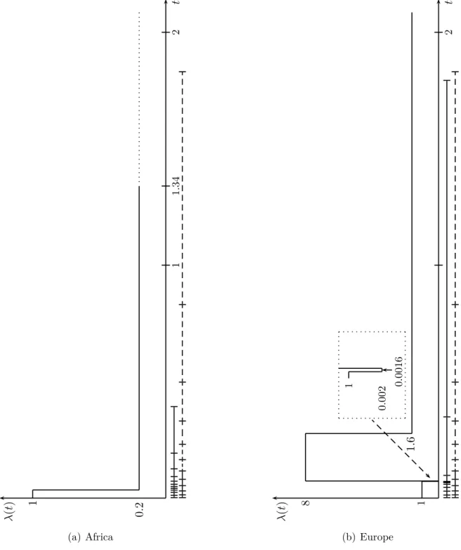
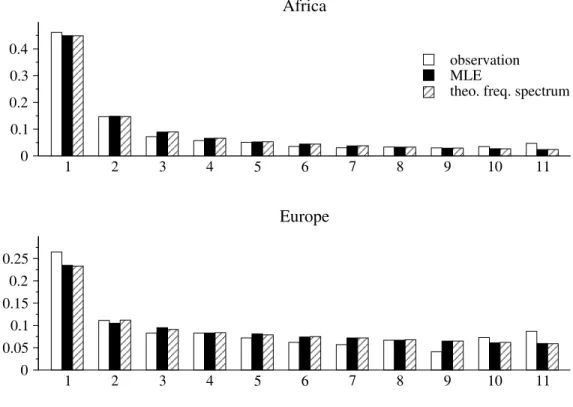
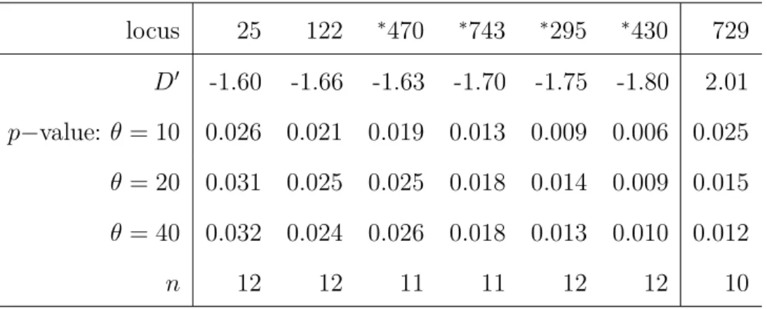
In Chapter 3, all revisited ( Griffiths and Tavaré 1998, 2003) and newly derived formulas regarding the first- and second-order moments of the size of a mutation and their corollaries are summarized into generalized versions of classical test statistics, which can be applied to test the neutral mutation hypothesis under variable population size to infer traces of selection. Since these test statistics assume an a priori knowledge of temporal changes in population size, it can only be applied if the necessary demographic parameters have been already estimated. Li and Stephan (2006) developed a maximum likelihood method to infer demographic changes and to detect recent selective sweeps in populations of varying size. The authors analyzed 262 and 272 X-linked loci from an African and a European population of D. melanogaster , respectively, and estimated their demographic histories based on the frequency spectra. First, we adapt the suggested demographic histories into the summary statistic D’—the generalization of Tajima’s D ( Tajima 1989b) to test the neutral mutation hypothesis under variable population size—

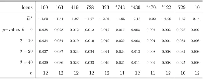
and analyze to what extent this test statistic can be used to infer the traces of selection on single loci. Innan and Stephan (2000) have addressed the same issue, using coales- cent simulations in order to distinguish the effects of exponential growth and selection in Arabidopsis thaliana . In analogy to the standard neutral version of Tajima’s D, the summary statistics of Fu and Li (1993) are able to be tested against the neutral non- equilibrium model. Even more pronounced than Tajima’s D, these test statistics measure an excess of singletons (i.e. site variants that occur once in a sample), which can either re- sult from exponential growth (Fu 1997), genetic hitchhiking (Kim and Stephan 2002), purifying selection ( Smith and Eyre-Walker 2002) or possibly by sequencing errors ( Achaz 2008) and should therefore be considered with caution. Exemplarily, we gener- alize one of these test statistics that relates the number of segregating sites, S n , to the number of singletons, but, as in the demographic history of the African population of D. melanogaster , this generalization may incorporate the impact of exponential growth, but may not distinguish positive from purifying selection or manage certain technological issues. Thereafter, a generalized version of the H test ( Fay and Wu 2000) is constructed to particularly measure an excess of high-frequency derived variants. Due to the prob- lematic interpretation of singletons, the chapter closes with a singleton-exclusive version of Tajima’s D, which is established in analogy to a recently proposed standard neutral version ( Achaz 2008).

It may be anticipated at this point, that the correction of the above mentioned test statistics for the African demography is well accomplishable, whereas the distributions of the standardized test statistics incorporating the European demography may be seen as too unsatisfactory for reliable inference. Interestingly, demographic parameter constella- tions, which were already critical for the use of test statistics that rely on the standard neutral model, remain cumbersome to some extent, when these are taken into account.

The classification of delicate demographic scenarios marks the beginning of Chapter 4.

We illustrate that the variance-to-mean ratio of total tree length (T c ), a simple measure

for the distortion of the distribution of T c and accordingly for S n , can be applied to

detect intractable population bottlenecks. Furthermore, we show that different models

of population size change typically lead to different frequency spectra. This question is

particularly important to assess whether it is sufficient to estimate a single one out of

numerously possible demographic parameter constellations. We conclude with an outline

of possible future research questions.

General coalescent trees

Throughout this chapter we investigate statistical measures, which reflect the ancestry of a sample of n genes, when recombination is absent. Griffiths and Tavaré (1998, 2003) have established the theoretical framework for general coalescent trees, which are specified as follows. Let T n , . . . , T 2 be the time periods during which the coalescent tree has n, . . . , 2 lineages, respectively. The general joint distribution of waiting times (T n , . . . , T 2 ) satisfies the assumptions that:

(A1) T n , . . . , T 2 are continuous random variables.

(A2) The ancestral tree is binary, and such that when there are k ancestral lines each pair has probability ^k ₂

of being the next pair to coalesce.

To model the effects of mutation on general coalescent trees, it is assumed that:

(A3) Conditional on the edge lengths of the tree, mutations occur according to independent Poisson processes of rate θ/2 along the edges of the tree.

While for the theoretical treatment of general coalescent trees generic time units are used, one time unit corresponds to 2N generations, where N is the current size of a diploid population, under variable population size. The compound parameter θ is given by θ = 4Nµ, where µ is the mutation rate per sequence per generation. Therefore, θ/2 is the mutation rate per sequence per 2N generations, providing the convenience of the same time scaling of the mutational and the genealogical process. Furthermore, mutations occur according to the infinitely-many-sites model, introduced earlier, under which the number of mutations in the genealogy of a sample of size n equals the number of segregating sites of these n sequences.

Griffiths and Tavaré (1998, 2003) have derived numerous analytical results for

general coalescent trees. Most notably, Griffiths and Tavaré (1998, 2003) have derived the frequency spectrum, which is the probability distribution q n,i of the number of times, i, a single mutation arising between the present and the time of the most recent common ancestor, is represented in the sample of size n, as µ → 0. The probability q n,i is given by

q n,i =

(n − i − 1)!(i − 1)! ⁿ⁻ⁱ⁺¹ P

k=2

k(k − 1) ^n−k _i−1 E(T k ) (n − 1)!

P n k=2

kE(T k )

, 0 < i < n. (2.1)

Equation 2.1, which relates the probabilities q n,i to the expected lengths of coalescent waiting times T k , may be used to illustrate the hierarchy within general coalescent trees.

While the mean waiting times of T k appear symbolically in Equation 2.1, the usage of Equation 2.2 provides an explicit result of the frequency spectrum under variable popu- lation size. For the standard neutral model, which represents the simplest special case of a general coalescent tree, replacing E(T k ) by ^k ₂

results in q n,i = i

n−1 P

k=1

k

.

2.1 Variable population size

We measure time backwards in units of 2N generations, where N is the size of a diploid population at time of sampling. Define λ N (t) = N (t)/N as the ratio of the population sizes at time t in the past and the present. Furthermore, let λ(t), which arises as the limit as N → ∞ to ensure that the population size becomes large in each generation and is supposed to be strictly positive for all t > 0, be real and piecewise continuous. The population-size intensity function Λ is defined by

Λ(t) = Z t

0

1 λ(u) du.

We assume that Λ(∞) = ∞, so that a sample of genes has a most recent common ancestor (MRCA) with probability 1.

The joint density ( Griffiths and Tavaré 1994) of (T n , . . . , T ₂ ) is g(t n , . . . , t 2 ) =

Y n

j=2

j 2

1

λ(s j ) exp{−

j 2

(Λ(s j ) − Λ(s j+1 ))},

for 0 ≤ t n , . . . , t 2 < ∞, where s n+1 = 0, s n = t n , s j = t j + . . . + t n , j = 2, . . . , n − 1.

Although the waiting times T n , . . . , T 2 are not independent, unlike in the case of con-

stant population size, where g(t n , . . . , t 2 ) = g (t n ) . . . g(t 2 ), we will use the joint density

and the law of iterated expectations to derive the first two moments of waiting times.

Griffiths and Tavaré (1998) already obtained the means based on previous results from Griffiths (1980) and Tavaré (1984). To emphasize the dependence of the first- and second-order moments of waiting times on the sample size n, waiting times and densities carry an index, n, unless the meaning is clear from the context.

2.1.1 Mean waiting times

First, we prove two lemmas.

Lemma 2.1.

Z

0

t

j 2

λ(t) exp{−

j 2

Z ^t

0

1

λ(u) du}dt = Z

0

exp{−

j 2

Z ^t

0

1

λ(u) du}dt.

Proof.

Z

0

t

j 2

λ(t) e

(

)

0 1 λ(u)

du

dt = − Z

0

t ( d

dt e

(

)

0 1 λ(u)

du

)dt = (integration by parts)

−( lim

t→∞ t e

(

)

0 1 λ(u)

du

− 0)

| {z }

=0

+ Z

0

e

(

)

0 1 λ(u)

du

dt.

2 In the last line of the proof, the assumption of Λ(∞) = ∞ is necessary to ensure that the limit for t → ∞ is zero.

Lemma 2.2.

Z

0

Z

0

n+1 2

λ(t n+1 ) exp{−

n + 1 2

^t Z

0

1

λ(u) du} exp{−

j 2

^t

Z ^+t

t

1

λ(u) du}dt _n+1 dt =

n+1 2

n+1 2

− ^j ₂



 Z

0

exp{−

j 2

Z ^t

0

1

λ(u) du}dt − Z

0

exp{−

n + 1 2

Z ^t

0

1

λ(u) du}dt



 .

Proof.

Z

0

Z

0

n+1 2

λ(t n+1 ) e

(

)

0 1 λ(u)

du

e

−

(

)

R t

tn+1 1 λ(u)

du

dt _n+1 dt = (substitute t _n+1 + t by s) Z

0

Z s

0

n+1 2

λ(t _n+1 ) e

(

)

0 1 λ(u)

du

e

−

(

)

tn+1 1 λ(u)

du

dt n+1 ds =

n+1 2

n+1 2

− ^j ₂ Z

0

Z s

0 n+1

2

− ^j ₂

λ(t n+1 ) e

(

)

(

) ⁾

0 1 λ(u)

du

e

(

)

0 1 λ(u)

du

dt n+1 ds =

n+1 2

n+1 2

− ^j ₂ Z

0

e

(

)

0 1 λ(u)

du



 Z s

0 n+1

2

− ₂ ^j

λ(t n+1 ) e

(

)

(

) ⁾

0 1 λ(u)

du

dt n+1



 ds =

n+1 2

n+1 2

− ^j ₂ Z

0

e

(

)

0 1 λ(u)

du



 Z s

0

(− d dt n+1

e

(

)

(

) ⁾

0 1 λ(u)

du

)dt _n+1



 ds =

n+1 2

n+1 2

− ^j ₂ Z

0

e

(

)

0 1 λ(u)

du

1 − e

(

)

(

) ⁾

0 1 λ(u)

du !

ds = (rename s by t)

n+1 2

n+1 2

− ^j ₂



 Z

0

e

(

)

0 1 λ(u)

du

dt − Z

0

e

(

)

0 1 λ(u)

du

dt



 .

2

The following chart illustrates the setup of recursions and the way of inductive reasoning.

E(T 2 ) 2

&

E(T 3 ) 3 E(T 2 ) 3

& &

E(T 4 ) 4 E(T 3 ) 4 E(T 2 ) 4

& & &

· · · · · · · · · · · · E(T k ) n

&

E(T k ) n+1

Now, we start to successively derive E(T n ) n , E(T n−1 ) n , . . . and perform these recursions in particular for small sample sizes. From the joint density above one immediately obtains

E(T n ) n = Z

0

t n g n (t n )dt n = Z

0

t

n 2

λ(t) exp{−

n 2

Z t 0

1

λ(u) du}dt

= Z

0

exp{−

n 2

Z t 0

1

λ(u) du}dt,

by making use of Lemma 2.1. This result forms the initial step of the induction proof and provides in particular the solutions for E (T ₂ ) ₂ and E(T ₃ ) ₃ . To calculate E(T ₂ ) ₃ we use conditional expectations:

E(T ₂ ) ₃ = E(E(T ₂ |T ₃ ) ₃ ) = Z

0

g ₃ (t ₃ )E(T ₂ |T ₃ = t ₃ ) ₃ dt ₃

= Z

0 3 2

λ(t 3 ) exp{−

3 2

Z t

0

1

λ(u) du} Z

0

exp{−

2 2

Z t

+t t

1

λ(u) du}dt dt ₃ .

Note that the result for E(T 2 ) 2 is used on the right-hand side of the above equation. Due to conditioning on T 3 = t 3 , the integration bounds are shifted by t 3 . Using Lemma 2.2 we can continue and write

E(T 2 ) 3 =

3 2

3 2

− ² ₂ Z

0

exp{−

2 2

Z t 0

1

λ(u) du}dt − Z

0

exp{−

3 2

Z t 0

1

λ(u) du}dt .

In the same way, we obtain E(T _n−1 ) n =

X n

j=n−1

(−1) ^j+n−1 α _n,j,n−1 Z

0

exp{−

j 2

Z t 0

1

λ(u) du}dt, where

α n,j,n−1 =

n 2

n 2

− ⁿ⁻¹ ₂ .

Since this result provides us with the solution for E(T 3 ) 4 , we finally derive E(T 2 ) 4 by conditioning the result for E(T 2 ) 3 on the newly introduced waiting time T 4 .

E(T 2 ) 4 = E(E((T 2 ) 3 |T 4 ) 4 ) = Z

0

g 4 (t 4 )E((T 2 ) 3 |T 4 = t 4 ) 4 dt 4 = · · ·

=

3 2

3 2

− ² ₂

4 2

4 2

− ² ₂ Z

0

exp{−

2 2

Z t 0

1

λ(u) du}dt

−

3 2

3 2

− ² ₂

4 2

4 2

− ³ ₂ Z

0

exp{−

3 2

Z t 0

1

λ(u) du}dt +

3 2

3 2

− ² ₂

⁴

2

4 2

− ³ ₂ −

4 2

4 2

− ² ₂ Z

0

exp{−

4 2

Z t 0

1

λ(u) du}dt

= X 4

j=2

(−1) ^j+2 α 4,j,2

Z

0

exp{−

j 2

Z t 0

1

λ(u) du}dt.

In analogy, E(T n−2 ) n =

X n

j=n−2

(−1) ^j+n−2 α n,j,n−2

Z

0

exp{−

j 2

Z t 0

1

λ(u) du}dt, where

α n,j,n−2 =

n−1 2

n−1 2

− ⁿ⁻² ₂

n 2

n 2

− ^j ₂ , j = n − 1, n − 2, and α n,n,n−2 = α n,n−1,n−2 − α n,n−2,n−2 .

When performing the next recursion step to calculate E(T n−3 ) n , one might already see that

α n,k,k = Y n

i=k+1 i 2

i 2

− ^k ₂ = (2k − 1)!n!(n − 1)!

k!(k − 1)!(n − k)!(n + k − 1)! . The solutions of α n,k,k , α n,k+1,k , . . . eventually lead to

E(T k ) = X n

j=k

(−1) ^j+k α n,j,k

Z

0

t g j (t)dt, 2 ≤ k ≤ n, (2.2)

where

α n,j,k = (2j − 1)n!(n − 1)!(k + j − 2)!

(j − k)!k!(k − 1)!(n − j)!(n + j − 1)! , g j (t) =

j 2

λ(t) exp{−

j 2

Z ^t

0

1 λ(u) du},

and e.g., g 2 (t 2 ) is the density of (T 2 ) 2 . The proof of Equation 2.2 requires the following

combinatorial identity.

Lemma 2.3.

X n

j=k

(−1) ^j+k α n,j,k = 0.

Proof.

X n

j=k

(−1) ^j+k α n,j,k = X n

j=k

(−1) ^j+k (2j − 1) n!(n − 1)!(k + j − 2)!

k!(k − 1)!(n − j)!(n + j − 1)!(j − k)!

=

2k−2 k−2

(k − 1) ²ⁿ⁻¹ _n−1

X n

j=k

(−1) ^j+k (2j − 1)

2n − 1 n − j

k + j − 2 j − k

(upper negation of last term)

=

2k−2 k−2

(k − 1) ²ⁿ⁻¹ _n−1

X n

j=k

(−1) ^j+k (2j − 1)

2n − 1 n − j

(−1) ^j−k

1 − 2k j − k

=

2k−2 k−2

_2(n−k)

n−k

(k − 1) ²ⁿ⁻¹ _n−1

X n

j=k

((2j − 2k) + (2k − 1))

2n−1 n−j

_1−2k

j−k

2(n−k) n−k

=

2k−2 k−2

_2(n−k)

n−k

(k − 1) ²ⁿ⁻¹ _n−1 ×

2

X n

j=k

(j − k)

2n−1 n−j

_1−2k

j−k

2(n−k) n−k

+ (2k − 1) X n

j=k 2n−1

n−j

_1−2k

j−k

2(n−k) n−k

=

2k−2 k−2

_2(n−k)

n−k

(k − 1) ²ⁿ⁻¹ _n−1 ×

2(n − k) 1 − 2k 2(n − k)

X n

j=k 2n−1

n−j

j−k−1

2(n−k)−1 n−k−1

| {z }

=1

+(2k − 1) X n

j=k 2n−1

n−j

_1−2k

j−k

2(n−k) n−k

| {z }

=1

= 0.

2

In the penultimate line of the proof of Lemma 2.3, both sums are equal to one because

of Vandermonde’s convolution. Now we are ready to complete the proof of Equation 2.2.

Proof of Equation 2.2.

To infer E(T k ) n+1 from the induction assumption given in Equation 2.2, we write

E(T k ) n+1 = E(E(T k |T n+1 ) n+1 ) = Z

0

g n+1 (t n+1 )E(T k |T n+1 = t n+1 ) n+1 dt n+1

= Z

0

n+1 2

λ(t n+1 ) exp{−

n + 1 2

^t Z

0

1

λ(u) du}E(T k ) ^λ _n

dt n+1 ,

where (cf. Figure 2.1)

E(T k ) ^λ _n

= (induction assumption)

= X n

j=k

(−1) ^j+k α n,j,k

Z

0

t

j 2

λ s (u) exp{−

j 2

Z ^t

0

1

λ s (u) du}dt

= (Lemma 1) X n

j=k

(−1) ^j+k α n,j,k

Z

0

exp{−

j 2

Z ^t

0

1

λ s (u) du}dt

= (λ s (u) = λ(u + t n+1 )) X n

j=k

(−1) ^j+k α n,j,k

Z

0

exp{−

j 2

Z ^t

0

1

λ(u + t n+1 ) du}dt

= (substitute v = u + t n+1 ) X n

j=k

(−1) ^j+k α n,j,k

Z

0

exp{−

j 2

^t

Z ^+t

t

1

λ(v) dv}dt

= (rename v by u) X n

j=k

(−1) ^j+k α n,j,k

Z

0

exp{−

j 2

^t

Z ^+t

t

1

λ(u) du}dt.

Therefore,

E(T k ) n+1 = Z

0

n+1 2

λ(t n+1 ) e

(

)

0 1

λ(u)

du n

X

j=k

(−1) ^j+k α n,j,k

Z

0

e

−

(

)

R t

tn+1 1 λ(u)

du

dt

! dt n+1

= X n

j=k

(−1) ^j+k α n,j,k

Z

0

Z

0

n+1 2

λ(t n+1 ) e

(

)

0 1 λ(u)

du

e

−

(

)

R t

tn+1 1 λ(u)

du

dt n+1 dt.

0 t _n+1 t _n+1 + t u 0 t u

λ ( u ) ^{− 1} λ s ( u ) ^{− 1}

.. . .. . .. .

⇐⇒

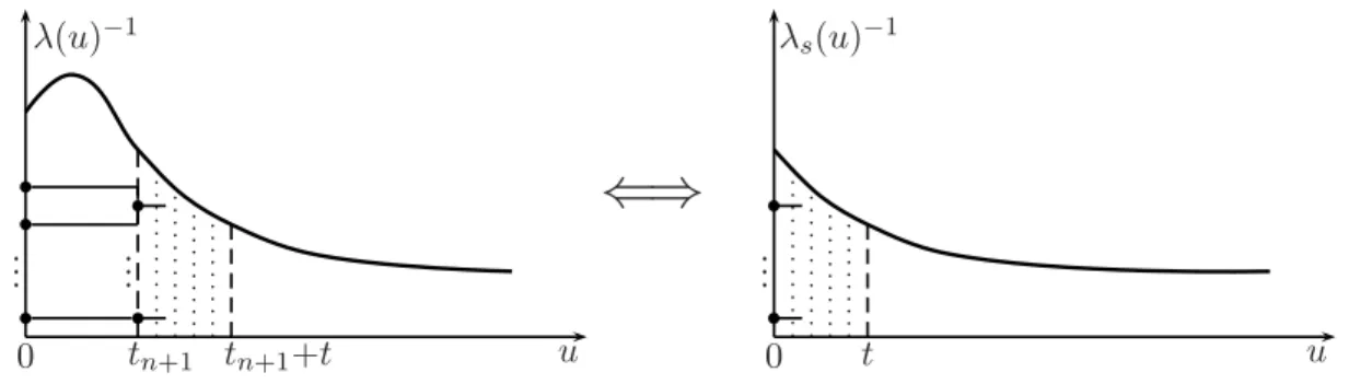
Figure 2.1 Since t n+1 is fixed within E(T k |T n+1 = t n+1 ), we can shift λ

by t n+1 to the left resulting in the function λ

_s with λ s (u)

= λ(u+t _n+1 )

. Without loss of generality, we can use Equation 2.2 with respect to λ

_s (denoted as E(T _k ) ^λ _n

) as our induction assumption as well.

By Lemma 2.2, we get E(T k ) _n+1 =

X n

j=k

(−1) ^j+k α n,j,k

n+1 2

n+1 2

− ^j ₂

| {z }

=α

( Z

0

e

(

)

0 1 λ(u)

du

dt − Z

0

e

(

)

0 1 λ(u)

du

dt).

The usage of Lemma 2.3 results in

E(T k ) n+1 = X n

j=k

(−1) ^j+k α n+1,j,k

Z

0

e

(

)

0 1 λ(u)

du

dt − X ⁿ⁺¹

j=k

(−1) ^j+k α n+1,j,k

| {z }

=0

−(−1) ^n+1+k α n+1,n+1,k

Z

0

e

(

)

0 1 λ(u)

du

dt

= X n+1

j=k

(−1) ^j+k α n+1,j,k

Z

0

e

(

)

0 1 λ(u)

du

dt.

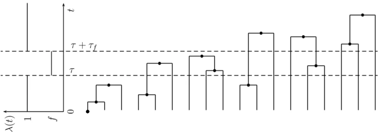
2 The expected waiting times for specific demographic scenarios can be derived from Equa- tion 2.2. Population genetical models which consider a finite number of instantaneous population size changes can be explicitly solved, as seen in the following example of a population bottleneck (cf. Figure 2.2). Let λ(t) = f for τ ≤ t < τ + τ f and λ(t) = 1 otherwise. Then,

E(T k ) = X n

j=k

(−1) ^j+k α n,j,k

1

j 2

(1−(1−f)(exp{−

j 2

τ }−exp{−

j 2

(τ + τ f

f )})), 2 ≤ k ≤ n.

t 0

λ ( t ) 1 f

τ τ + τ

Figure 2.2 Possible coalescent trees for a 3-phase bottleneck model and sample size n = 3.

In the case of exponential growth, where λ(t) = exp{−βt} and β > 0, the mean waiting times E(T k ) can be expressed in terms of the exponential integral Ei(.) and are

E(T k ) = − X n

j=k

(−1) ^j+k α n,j,k

1 β exp{

j 2

β } Ei(−

j 2

β ), 2 ≤ k ≤ n.

Obviously, the assumption of a large population size in each generation is violated at some time in the past. However, the upper equation yields the same result as if we would perform a logarithmic time-scale transformation ( Griffiths and Tavaré 1998) to the Kingman coalescent ( Kingman 1982b). Models of instantaneous population size change followed by exponential growth can be expressed in terms of tabulated functions as well.

2.1.2 Mean squared waiting times

The same ideas of using conditional expectations and a proof by induction can be applied to the second-order moments of waiting times. To derive the mean squared waiting times E(T _k ² ), we first show the following Lemma.

Lemma 2.4.

Z∞

0

Z∞

0

Z∞

0

t

`_n+1

2

´

λ(t

)

`_j

2

´

λ(t

+ t

)

`_k

2

´

λ(t

+ t

+ t) e

−“_n+1 2

”^tn+1 R 0

1 λ(u)du

e

−“_j 2

”^tn+1+t 0 R tn+1

1 λ(u)du

e

−“_k 2

”^tn+1+t 0+t R

tn+1+t0 1 λ(u)du

dt

dt

dt

`_n+1

2

´

`_n+1

2

´−`j 2

´ Z∞

0

Z∞

0

t

`j 2

´

λ(t

)

`k 2

´

λ(t

+ t) e

−“_j 2

”t0 R 0

1 λ(u)du

e

−“_k 2

”t0+t R t0

1 λ(u)du

dt

dt

`j 2

´

`n+1 2

´−`j 2

´ Z∞

0

Z∞

0

t

`n+1 2

´

λ(t

)

`k 2

´

λ(t

+ t) e

−“_n+1 2

”t0 R 0

1 λ(u)du

e

−“_k 2

”^t0R^+t t0

1 λ(u)du

dt

dt.

Proof.

Z∞

0

Z∞

0

Z∞

0

t

`_n+1

2

´

λ(t

)

`_j

2

´

λ(t

+ t

)

`_k

2

´

λ(t

+ t

+ t) e

−“_n+1 2

”^tn+1 R 0

1 λ(u)du

e

−“_j 2

”^tn+1+t 0 R tn+1

1 λ(u)du

e

−“_k 2

”^tn+1+t 0+t R

tn+1+t0 1 λ(u)du

dt

dt

dt

(substitute t n+1 + t

+ t by s 2 and t n+1 + t

by s 1 , respectively)

Z∞

0 s₂

Z

0 s₁

Z

0

(s

s

)

`_n+1

2

´

λ(t

)

`_j

2

´

λ(s

)

`_k

2

´

λ(s

) e

−“_n+1 2

”^tn+1 R 0

1 λ(u)du

e

−“_j 2

” ^s1 R tn+1

1 λ(u)du

e

−“_k 2

”^s2 R s1

1 λ(u)du

dt

ds

ds

Z∞

0 s2

Z

0

(s

s

)

`j 2

´

λ(s

)

`k 2

´

λ(s

) e

−“_j 2

”^s1 R 0

1 λ(u)du

e

−“_k 2

”^s2 R s1

1

λ(u)du `_n+1

2

´

`n+1 2

´−`j 2

´×

s1

Z

0

`_n+1

2

´−`j 2

´

λ(t

) e

−(“_n+1 2

”

−“_j 2

” )

tn+1 R 0

1 λ(u)du

dt

!

| {z }

=

−

s1

R

0 d

dt_n+1

e

(

)

(

)

0 1 λ(u)du

dt

ds

ds

Z∞

0 s2

Z

0

(s

s

)

`j 2

´

λ(s

)

`k 2

´

λ(s

) e

−“_j 2

”^s1 R 0

1 λ(u)du

e

−“_k 2

”^s2 R s1

1

λ(u)du `_n+1

2

´

`_n+1

2

´−`j 2

´

1

e

−(“_n+1 2

”−“_j 2

”) s1

R 0

1 λ(u)du!

ds

ds

`_n+1

2

´

`_n+1

2

´−`j 2

´ Z∞

0 s₂

Z

0

(s

s

)

`_j

2

´

λ(s

)

`_k

2

´

λ(s

) e

−“_j 2

”^s1 R 0

1 λ(u)du

e

−“_k 2

”^s2 R s1

1 λ(u)du

ds

ds

`j 2

´

`_n+1

2

´−`j 2

´ Z∞

0 s2

Z

0

(s

s

)

`_n+1

2

´

λ(s

)

`k 2

´

λ(s

) e

−“_n+1 2

”^s1 R 0

1 λ(u)du

e

−“_k 2

”^s2 R s1

1 λ(u)du

ds

ds

(introduce s ₂ − s ₁ = t, rename s ₁ by t

, replace s ₂ by t

+ t)

`_n+1

2

´

`n+1 2

´−`j 2

´ Z∞

0

Z∞

0

t

`j 2

´

λ(t

)

`k 2

´

λ(t

+ t) e

−“_j 2

”t0 R 0

1 λ(u)du

e

−“_k 2

”t0+t R

t0 1 λ(u)du

dt

dt

`_j

2

´

`_n+1

2

´−`_j

2

´ Z∞

0

Z∞

0

t

`_n+1

2

´

λ(t

)

`_k

2

´

λ(t

+ t) e

−“_n+1 2

”t0 R 0

1 λ(u)du

e

−“_k 2

”^t0R^+t t0

1 λ(u)du

dt

dt.

2

The following chart illustrates the setup of recursions and the way of inductive reasoning.