A Unified Model of Non-Panmictic Population Structures in Evolutionary Algorithms

REIHE COMPUTATIONAL INTELLIGENCE

COLLABORATIVE RESEARCH CENTER 531

Design and Management of Complex Technical Processes and Systems by means of Computational Intelligence Methods

A Unied Model of Non-Panmictic Population Structures in Evolutionary Algorithms

Joachim Sprave No. CI-55/99

Technical Report ISSN 1433-3325 January 1999

Secretary of the SFB 531

University of Dortmund

Dept. of Computer Science/XI 44221 Dortmund

Germany

This work is a product of the Collaborative Research Center 531, \Computational

Intelligence", at the University of Dortmund and was printed with nancial support of

the Deutsche Forschungsgemeinschaft.

1 Motivation

In most variants of Evolutionary Algorithms (EAs), multiple search points are considered each iteration.

In analogy to nature, the search points are called a population of (articial) individuals. Due to the fact that computers were slow and mostly sequential machines when these algorithms were developed, the inherent parallelism of populations had to be serialized in the rst implementations. Later on, when parallel computers became aordable for universities, researchers began to parallelize EAs again. Since the terminology of the sequential algorithms had more or less settled at that time, the parallel versions were described by an extension of the sequential terminology where a generalization would have been appropriate instead. Surprisingly, this generalization has not been done ever since, although there were approaches to a common terminology of parallel EAs. The work described here is an attempt to provide a unied model of population structures, independently of their parallelization properties. This paper starts with a brief overview of other approaches to model, classify, or analyze population structures. Then, a general framework for the formal description of population structures is introduced, followed by examples of common population structures expressed by means of the given model. Finally, as an application of the formal framework, a method for calculating growth rates and takeover times of arbitrary population structures is presented.

2 Parallelism and Population Structures

Traditional EAs allow each individual in a population to interact (compete or mate) with any other. In biological terms, a population like this is called panmictic . This fully connected interaction scheme is not very well suited for a parallel implementation.

On the other hand, parallelizing a sequential algorithm usually means that the parallel version, given the same input as the original algorithm,produces the same output, as well. Since every parallel algorithm can be run time sliced on a sequential machine, the maximum speed-up is limited linearly by the number of processors. In other words, parallelization does not change the quality of results, it just delivers the same results in less time.

Except for master/slave parallelization of tness function evaluations, all parallel EA approaches violate the same-input-same-output rule. The panmictic approach is replaced by structured populations which can be evaluated in parallel with a reduced need for communication.

First attempts to a unied terminology of non-panmictic population structures were made by Gorges- Schleuter [1], who presented a rough classication of parallel EAs. She identied three major models of parallelization in EAs:

Island Model:

The population consists of separated subpopulations. Each subpopulation is a panmictic EA. A limited amount of genetic information is exchanged between arbitrary subpopulations.

Stepping Stone Model:

The population consists of separated, panmictic subpopulations. A non-total neighborhood relation is dened on the subpopulations. A limited amount of genetic information is exchanged between adjacent subpopulations.

Neighborhood Model:

A non-total neighborhood relation is dened on the individuals. Individuals interact (mate, com- pete) with adjacent individuals only.

Today, most authors do not discriminate between the island and stepping stone model. Instead, either the term island model or migration model is used for an EA with panmictic subpopulations. The neighborhood model is sometimes also called diusion model.

In the past, work on population structures always emphasized a particular model. For panmictic

subpopulations, there are mostly empirical studies, e.g. [2, 3, 4, 5]. In a theoretical approach, Cantu-Paz

[6] presented optimal subpopulation sizes for some special instances of Genetic Algorithms.

Neighborhood models were analyzed with respect to local selection schemes [7, 8] as well as neighbor- hood shapes in grid topologies [9, 10].

3 A Hypergraph-Based Model of Population Structures

3.1 Hypergraphs

The denitions in this section base on the theory of hypergraphs as dened by Berge [11] in the 60s.

E2 E1

E3

E4

10 2

1 3

4

7 5

6

9 8

Figure 1: A hypergraph with vertices X =

1;:::;10

and edges E

=

1;2;3;4

, E

=

2;4;7;8

, E

=

8;9;10

, and E

=

3;4;5;6;7

.

Graphs are usually dened as sets of pairs of a base set. Elements of the base set are called vertices , and pairs of vertices are called edges . The basic idea of hypergraphs is the extensions of edges from pairs to arbitrary subsets of the set of vertices:

Def. 1

Let be X =

x

;x

;:::;x n

a nite set, and

= (E i

i

I) a family of subsets of X. The family

E

is called hypergraph on X, if

E i

=

i

I (1)

[

i

I E i = X : (2)

The pair H = (X;

) is called hypergraph, and

X

is the order of H.

Two vertices x k and x l of an hypergraph are adjacent , if they are contained in common edge, formally

9

i : x k

E i

x l

E i : (3)

For each hypergraph H = (X;

), there exists a dual Hypergraph H

= (E;

), with vertices e

;:::;e _m and edges

X

;:::;X _n

, given that:

8

j

1;:::;n

: X j =

e i

i

m;E i

x j

, (4)

where the vertices e i correspond with the edges E i of H, and the edges X j with the vertices x j of H,

respectively.

3.2 Representations of Hypergraphs

The eciency of algorithmson simple graphs is usually based on a suitable representation of a given graph.

Many algorithms are dened on adjacence lists or adjacence matrices. These representations cannot be easily transfered to hypergraphs, because the information which edge two vertices are connected by is lost.

A loss-free representation of a hypergraph is its incidence matrix. The columns of the matrix represent the edges of the hypergraph and the lines the vertices. If H is a hypergraph with edges m and vertices n, then it is described by the matrix A with

a _i;j =

(

1 if x i

E j

0 else. (5)

The indicidence matrix of the hypergraph given in Fig. 1 is

A =

0

B

B

B

B

B

B

B

B

B

B

B

B

B

B

B

B

B

B

B

B

@

1 0 0 0 1 1 0 0 1 0 0 1 1 1 0 1 0 0 0 1 0 0 0 1 0 1 0 1 0 1 1 0 0 0 1 0 0 0 1 0

1

C

C

C

C

C

C

C

C

C

C

C

C

C

C

C

C

C

C

C

C

A

The adjacence of two vertices x i and x k can be calculated as scalar product of the ith that kth row:

< a i;

;a k;

>= 1

E j : x i

E j

x k

E j : (6) The vertex adjacence matrix B with b i;k =< a i;

;a k;

> can be obtained as follows:

B = AA

(7)

Accordingly one can express the edge adjacence matrix as scalar product of the appropriate lines of the incidence matrix. One receives the matrix as

B

= A

A: (8)

B

is as well the vertex adjacence matrix of the dual hypergraph H

. The matrix B

, for example, allows the calculation of the diameter with

(H) = min

k

^k

i

B

ⁱ = K n

(9)

where K n is the adjacence matrix of the complete (simple) graph with n vertices.

3.3 Modeling of Population Structures by Means of Neighborhood Graphs

Non-panmictic population models, as published in the past, usually base on regular geometric structures.

Frequently, rings, tori, or cubes are used to place the individuals or subpopulations on. Since all these

structures can be described as meshes, there is already a natural notion of adjacency. For neighborhood models, the most popular population layout is a two-dimensional grid folded to a torus.

The neighborhood relation in torus shaped populations is not necessarily limited to adjoining mesh point, but it is more often dened by means of a distance measure in a two-dimensional plane. Clearly, once the neighborhood relation is given, it can be represented by a graph. While a graph representation seems to be appropriate for neighborhood models, it does not very well reect the structure of coarse grained models. A neighborhood graph of a migration model contains large cliques, i.e. fully connected subgraphs. A formal denition of populations structures by means of graphs is omitted here in favor to the following, more general model which is based on the theory of hypergraphs.

4 Modeling of Population Structures by Means of Hypergraphs

4.1 Denitions

Before we give a denition of population structures, we must state what a population is in this context:

Def. 2

Let be A the search space of a given objective function, S the space of additional state information needed by the optimization algorithm under consideration. Then an element of the family A

S is called an individual . A family of individuals (p ^t

;:::;p _t

);p _ti

A

S is called population at time t or population at generation t.

The state information may contain, e.g., the mutation variances of an Evolution Strategy.

Since the actual values of individuals are not needed for the denition of population structures, it is sucient to identify individuals by their indices in the population.

Def. 3

A population structure on a population P with

P

= is a triple (X;

;

), consisting of a hypergraph (X;

);X =

0;:::;

1

;

(X), and a partition

(

) of X with

=

. The hyperedge E _i is called deme of the elements from Q _i

.

As the term deme indicates, each hyperedge contains the potential parents of the individuals in the corresponding element of the partition. The duality of hypergraph is also reected by the denition of population structures. Since the partition

can be also interpreted as a hypergraph, there are two matrices associated with population structures:

E

IB

^m

: Incidence matrix of the hypergraph (X;

).

Q

IB

^m

: Incidence matrix of the hypergraph (X;

).

Consider the relation i is a potential parent of j. The adjacence matrix of the associated simple graph can be written as

A = E Q

IB

; =

X

(10)

. Lets calls this matrix the individual adjacence matrix. The dual matrix, the deme adjacence matrix, describes the relation Q i has potential ospring in Q j . It can be calculated as

A

= Q

E

IB

^m

^m

; m =

(11)

As can be seen, this modeling approach adjusts to the scale of a particular population structure.

Def. 4

A path from i to j in a population structure = (X;

;

) is a nite sequence of 2-tuples (i ;j ); = 0;:::;l with i

= i;j l = j; and i

Q k

j

E k ;1

l. The value l is the length of the path (i ;j ).

If there exists a path from i to j, there is at least one shortest path. The longest shortest path

between two individuals is called the diameter of the population structure. Obviously, the diameter is as

well the elitist takeover time of a population structure. The diameter can be calculated as the diameter

of the simple graph G with (x;y)

G if

ZZ : x

E

y

Q . Let be E the incidence matrix

of H = (X;

), Q the incidence matrix of J = (X;

). Since g i;j =

^N _i

e x;i

q _i;y =< h x;

;q

;y >, the

adjacence matrix of G is E Q

.

5 Hypergraph Models of Population Structures

5.1 Panmixis

The most common population structure in Evolutionary Algorithms is panmictic:

pan = (X;

;

) X = (0;:::;

1)

Q

= (X)

E

= (X)

(12)

5.2 Migration and Pollination

In the following, the population structure of a migration model without isolation is presented. Let be P =

0;:::;

1

;

IN a population, r

IN the number of subpopulations with = r; r;

IN, and m

1;:::;

the number of migrants between adjacent subpopulations. The subpopulations are Q i =

i;:::;i +

1

;i = 0;:::;r

1.

Let be M s

t the set of migrants from subpopulation Q s to subpopulation Q t . If M s

t

=

, there is a migration path from Q s to Q t .

A proper model of migration does not keep the migrants in their source subpopulation after migration, i.e. the migrants are not in the set of potential parents of their successors. This is modeled by subtracting the set of migrants from their source populations hyperedge. The migration model can now be described as follows:

migr = (X;

;

)

X = (0;:::;

1)

Q i =

i;:::;i +

1

E

= (E

;:::;E _r

)

E i = Q i

r s

M s

i

r t

M i

t ; M s

i

Q s ; M i

t

Q i

(13)

If the subtraction of the migrants is omitted, one obtains a pollination model:

poll = (X;

;

) X = (0;:::;

1) Q i =

i;:::;i +

1

E

= (E

;:::;E r

)

E i = Q i

r s

M s

i ; M s

i

Q s

(14)

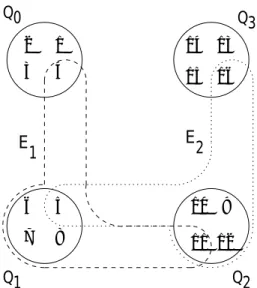
The dierence to the model above is that the migrants are also potential parents of the next generation of their source subpopulation. Since genetic information is copied instead of moved, the biological analogy of plants spreading pollen is more accurate than that of migrating animals. A pollination model is sketched in Fig. 2, with

X =

0;:::;15

Q

=

0;:::;3

;

4;:::;7

;

8;:::;11

;

12;:::;15

E

=

0;:::;3;5;14

;

4;:::;7;3;10

;

8;:::;11;4;15

;

12;:::;15;0;9

(15)

Q3

Q1 Q2

Q0

E 1 E

2

3 4

7 8 2 1

5

6 10 9

11 12 13 14 15 16

Figure 2: Sketch of a pollination population structure with four subpopulations in a ring. For the sake of clarity, the hyperedges E

and E

are omitted.

5.3 Fine Grained Models

The majority of the ne grained approaches published in literature uses grid or torus topologies. The neighborhood relation is derived from a topological measure. A simple yet widely used topology, a one-dimensional ring with individuals and a neighborhood radius of , is described by the following population structure:

ring = (X;

;

) X = (0;:::;

1)

Q

= (

x

;:::;

x

)

E

= (E

;:::;E

) E i = (i

;:::;i + )

(16)

where

and + are calculated in the factor group ZZ. Examples for symmetrical contiguous neighbor- hoods on two-dimensional meshes are given in [9] and [10].

The mapping of populations in the two-dimensional Euclidean plane usually results from biological analogies[1], in some cases indirectly by the notion of cellular automata[12]. Actually, grid induced neighborhoods are just special cases of graph induced neighborhoods. For a given maximum distance , any connected graph G

X

X induces the following population structure:

graph = (X;

;

)

X = (0;:::;

1)

Q

= (

x

;:::;

x

)

E

= (E

;:::;E

)

E i =

j

d G (e i ;e j )

; 1

=2

(17)

where d _G (x;y) is the length of the shortest path from x to y in G.

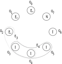
A simple neighborhood model is sketched in Fig. 3, with X =

0;:::;15

Q

=

0

;

1

;

2

;

3

;

4

;

5

;

6

;

7

E

=

7;0;1

;

0;1;2

;

1;2;3

;

2;3;4

;

3;4;5

;

4;5;6

;

5;6;7

;

6;7;0

(18)

E4 E3

1

0

7

6

5 2

4 3

Q2 Q1

Q3

Q4

Q5 Q6 Q7 Q0

Figure 3: Sketch of a neighborhood population structure with eight individuals in a ring. For the sake of clarity, only the hyperedges E

and E

are drawn.

5.4 Fine Grained Models

6 Modeling Isolation Times

The denition of population structures given above does not allow the modeling of isolation times. Using edge weights as in classical ow problems results in a cumulation over the time, averaging out some of the eects of isolation. Therefore, the given denition is extended not only to allow isolation, but any change of the population structure over time. This is achieved by replacing the hypergraph H by a sequence of hypergraphs H ^t ;t

IN, where (X;

^t ;

) is the population structure applied to generate generation number t + 1 from generation number t.

Def. 5

A dynamic population structure on a population P with

P

= is a triple (X;

^t ;

), consisting of a sequence of hypergraphs H ^t = (X;

^t ); X =

0;:::;

1

;

t

(X) and

t

IN :

^t

= m, as well as a partition

(

) of X with

= m. The hyperedge E _ti is called deme at generation t of the elements of Q _i

. A dynamic population structure with

^t =

= const for all t

IN is called static population structure oder just population structure .

Def. 6

The diameter of a dynamic population structure is min

k

^k _i

ⁱ

A (t) = K

with A (t) =

H _t Q.

The pollination model from Eqn. 14 can now be extended by an isolation time : poll = (X;

^t ;

)

X = (0;:::;

1) Q i =

i;:::;i +

1

E

t = (E

^t ;:::;E _tr

) E _ti =

(

Q i

s;i

G M s

i ; M s

i

Q s for t

0 mod

Q i else

(19)

7 Takeover Behavior of Population Structures

In the last years, a growing number of researchers in eld of EAs try to nd good measures for the selection pressure of dierent selection methods. Some of them are biologically inspired, e.g. [13, 14, 15], others base on pure probability theory, e.g. [16, 17, 18]. A decent analysis of properties of panmictic selection methods was given by Blickle and Thiele [19].

All these approaches relay on the assumption that individuals are indistinguishable and interchange- able. Since this does not hold true for structured populations, the theory developed for panmictic populations cannot be easily transfered.

7.1 Takeover Times and Probabilities

A common analytical approach to measure the selection pressure of an EA is the calculation of the takeover time, i.e. the number of generations it takes for the best individual of the initial population to ll the entire population under selection only. Unfortunately, for non-elitist selection operators, there is always a positive probability that the best individual gets lost before the population could be taken over, especially in the beginning.

An improvement of this approach is the notion of a takeover probability[18]. The idea is to dene a Markov chain where each possible number of best individuals is an element of the state space.

Let be p select : IN

IN

IR;(;k)

p select (;k) a function calculating the success probability for a single trial if a population of individuals contains k best individuals, where success means drawing a best individual. Since selection of individuals is a Bernoulli experiment, the transition probability from a non-absorbing state i of the Markov chain into another state j is

p i;j =

j

(p select (i;)) ^j (1

p select (i;))

^j (20)

Because every trial has the same success probability, the success is binomial distributed. In the non- panmictic case, individuals are selected from dierent subsets of the population, thus trials have dierent success probabilities. Since this leads to a generalized binomial distribution, the state space of a Markov chain would be of size

_k

_k

. Thus, a Markov chain analysis as in [18] is practically impossible.

7.2 Probabilistic Diameter

Although a simplication with respect to the extinction of the best individual, the takeover time as dened in [17] can be useful to compare selection methods among each other. The scenario for takeover time calculations is the following: The initial population contains a single best individual. Then, only selection is applied until the entire population consists of best individuals. The number of iterations needed is called the takeover time.

Section 6 contains the denition of the diameter of a population structure. Since the diameter is just the elitist takeover time of the population structure, it seems reasonable to calculate the takeover for non-elitist selection schemes in a similar manner. The idea is to propagate the best individual through the population as in the diameter calculation, based on the probability distribution of the selection operator.

Chakraborty et.al. [18] calculated the success probabilities for the most common selection operators.

Starting with a single best individual in the initial population, the expectation value of the number of best individuals after one generation is

E

_best :=

p select (;1) (21)

In general, for a given number k

^t

of best individuals in generation t,

E

_best ^t

:=

p select (;k

^t

) (22)

is the expectation value for the number of best individuals in generation t + 1. We obviously cannot calculate the expected number of best individuals in generation t by iterating eqn. 21 with

k

^t

:= E

_best ^t

(23)

This would mean to replace an iterated Bernoulli experiment by its expectation value. But then, this is how growth curve analysis and takeover time calculation was done in the past (e.g. [17], p. 71, eqn. 4).

To avoid the misleading notion of an expectation value, the following denition is given.

Def. 7

Let be = (X;

;

);

X

= a population structure, and p select : IN

IN

IR;(;k)

p select (;k) a success function for a given selection operator. Let be for all i

X:

s

_i = 1= (24)

r _ti =

j

E

s _tj ; i

Q (25)

s

_i ^t

= p select (r _ti ;

E

); i

Q (26)

The probabilistic diameter of under p _select is

" (;p select ) := min

t :

i

X : s

_i ^t

1

"

(27) The value 1

" is the required takeover level, where " is usually almost zero.

The recursive calculation of ~r ^t = (r ^t

;:::;r _t

) can be done simultaneously:

~r ^t = ~s

^t

E

^t

: (28) The value of min

s

_i ^t

i

X

can be interpreted as a growth coecient of the best individual. Fig. 4 shows the growth rates for panmictic population models with population size 1024 for linear ranking selection as well as (;)-selection. As in [17], the growth curves resemble logistic functions, in contrast to the growth curves of non-panmictic population models.

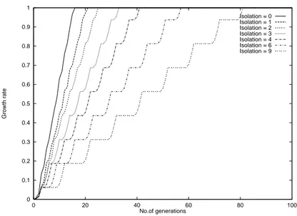
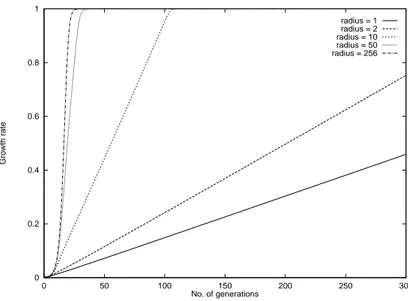
The growth curves of the migration models in Fig. 5 and Fig. 6 show the dierent reaction of (;) selection and linear ranking to isolation times. The latter keeps the logistic character for much higher isolation times. The curve of the neighborhood model in Fig. 7 shows the expected linear growth rates.

8 Conclusions and Outlook

This paper presents a unied model of population structures in Evolutionary Algorithms. It has been shown that the model is a powerful framework for calculations on non-panmictic populations. As an example, we have presented a denition of the takeover time of arbitrary population structures which is consistent with the traditional panmictic takeover time denition.

This model presented here is intended as a base for further theoretical work in the eld of non-

panmictic population structures. While a Markov chain model of non-panmictic population structures is

not generally useful, it should be possible to keep the state space small for a small number of demes by

taking advantage of the duality of the given denition. This is subject to further research.

0 0.1 0.2 0.3 0.4 0.5 0.6 0.7 0.8 0.9 1

0 20 40 60 80 100

Growth rate

No. of generations

(128,1024)-Selektion (256,1024)-Selektion (512,1024)-Selektion (768,1024)-Selektion Linear Ranking (max=2.0) Linear Ranking (max=1.5) Linear Ranking (max=1.1)

Figure 4: Growth curves of a panmictic (;) selection and linear ranking.

0 0.1 0.2 0.3 0.4 0.5 0.6 0.7 0.8 0.9 1

0 20 40 60 80 100

Growth rate

No.of generations

Isolation = 0 Isolation = 1 Isolation = 2 Isolation = 3 Isolation = 4 Isolation = 6 Isolation = 9

Figure 5: Growth curves of a migration model in a ring of 16 subpopulations and local (16,64) selection.

0 0.1 0.2 0.3 0.4 0.5 0.6 0.7 0.8 0.9 1

0 20 40 60 80 100

Growth rate

No. of generations

Isolation = 0 Isolation = 1 Isolation = 2 Isolation = 3 Isolation = 4 Isolation = 6 Isolation = 9

Figure 6: Growth curves of a migration model in a ring of 16 subpopulations and local linear ranking selection.

0 0.2 0.4 0.6 0.8 1

0 50 100 150 200 250 300

Growth rate

No. of generations

radius = 1 radius = 2 radius = 10 radius = 50 radius = 256

Figure 7: Growth curves of a neighborhood model in a ring of size 1024 and linear ranking selection (max

= 1.5).

Acknowledgments

This work is a product of the Collaborative Research Center Computational Intelligence (SFB 531).

Financial support by the Deutsche Forschungsgemeinschaft (DFG) is gratefully acknowledged.

References

[1] M. Gorges-Schleuter. Genetic Algorithms and Population Structures | A Massively Parallel Algo- rithm . Dissertation, Universitat Dortmund, 1990.

[2] J. P. Cohoon, S. U. Hedge, W. N. Martin, and D. S. Richards. Punctuated Equilibria: A Parallel Genetic Algorithm. In Grefenstette [20], pages 148{154.

[3] Ch. C. Pettey, M. R. Leuze, and J. J. Grefenstette. A Parallel Genetic Algorithm. In Grefenstette [20], pages 155{161.

[4] R. Tanese. Parallel Genetic Algorithm for a Hypercube. In Grefenstette [20], pages 177{183.

[5] Gunter Rudolph. Global optimization by means of distributed evolution strategies. In H.-P. Schwefel and R. Manner, editors, Parallel Problem Solving from Nature { Proc. First Workshop PPSN , pages 209{213, University of Dortmund, October 1{3, 1990. Springer, Berlin, 1991.

[6] Erick Cantu-Paz and David E. Goldberg. Predicting Speedups of Ideal Bounding Cases of Parallel Genetic Algorithms. In Thomas Back, editor, Proceedings of the 7th International Conference on Genetic Algorithms , pages 113{120, San Francisco, July19{23 1997. Morgan Kaufmann.

[7] Martina Gorges-Schleuter. ASPARAGOS An Asynchronous Parallel Genetic Optimization Strategy.

In J. David Schaer, editor, Proceedings of the 3rd International Conference on Genetic Algorithms , pages 422{427, George Mason University, June 1989. Morgan Kaufmann.

[8] Joachim Sprave. Linear neighborhood evolution strategy. In A. V. Sebald and L. J. Fogel, edi- tors, Proc. Third Annual Conf. Evolutionary Programming (EP'94) , pages 42{51, San Diego CA, February 24{26, 1994. World Scientic, Singapore.

[9] Gunter Rudolph and Joachim Sprave. Signicance of locality and selection pressure in the grand deluge evolutionary algorithm. In H.-M. Voigt, W. Ebeling, I. Rechenberg, and H.-P. Schwefel, editors, Parallel Problem Solving from Nature { PPSN IV, Int'l Conf. Evolutionary Computation , pages 686{694, Berlin, 22.{26. September 1996. Springer, Berlin.

[10] J.A. Sarma. An Analysis of Decentralized and Spatially Distributed Genetic Algorithms . Dissertation, George Mason University, Fairfax, VA, 1998.

[11] Claude Berge. Graphs and hypergraphs. North-Holland mathematical library ; 6. North-Holland Publ. Comp., Amsterdam, 3. edition, 1973.

[12] Joachim Sprave. Zellulare evolutionare Algorithmen zur Parameteroptimierung. In R. Hofestadt, F. Kruckeberg, and T. Lengauer, editors, Informatik in den Biowissenschaften, 1. Fachtagung der GI-FG 4.0.2 , pages 111{120, Bonn, 15.{16. Februar 1993. Springer, Berlin.

[13] H. Muhlenbein and D. Schlierkamp-Voosen. Predictive Models for the Breeder Genetic Algorithm.

Evolutionary Computation , 1(1):25{49, 1993.

[14] D. Thierens and D. E. Goldberg. Convergence Models of Genetic Algorithm Selection Schemes.

In Y. Davidor, H.-P. Schwefel, and R. Manner, editors, Parallel Problem Solving from Nature |

PPSN III International Conference on Evolutionary Computation , volume 866 of Lecture Notes in

Computer Science , pages 119{129. Springer, Berlin, 1994.

[15] Th. Back. Generalized convergence models for tournament- and (,)-selection. In L. Eshelman, editor, Proceedings of the 6th International Conference on Genetic Algorithms , pages 2{8. Morgan Kaufmann Publishers, San Francisco, CA, 1995.

[16] A. E. Nix and M. D. Vose. Modeling genetic algorithms with Markov chains. Annals of Mathematics and Articial Intelligence , 5:78{88, 1992.

[17] D. E. Goldberg and K. Deb. A Comparative Analysis of Selection Schemes Used in Genetic Al- gorithms. In G. J. E. Rawlins, editor, Foundations of Genetic Algorithms , pages 69{93. Morgan Kaufmann Publishers, San Mateo, CA, 1991.

[18] U. K. Chakraborty, Deb, K., and M. Chakraborty. Analysis of Selection Algorithms: A Markov Chain Approach. Evolutionary Computation , 4(2):133{167, 1996.

[19] T. Blickle and L. Thiele. A Comparison of Selection Schemes Used in Evolutionary Algorithms.

Evolutionary Computation , 4(4):361{394, 1996.

[20] J. J. Grefenstette, editor. Proceedings of the Second International Conference on Genetic Algorithms

and Their Applications . Lawrence Erlbaum Associates, Hillsdale, NJ, 1987.