Mathematical Population Genetics

Mathematical Population Genetics

Lecture Notes

Joachim Hermisson

January 10, 2018 University of Vienna Mathematics Department Oskar-Morgenstern-Platz 1

1090 Vienna, Austria

Copyright (c) 2017 Joachim Hermisson. For personal use only - not for distribution. These lecture notes are based on previous course material from the “Population Genetics Tutorial”

by Peter Pfaffelhuber, Pleuni Pennings, and JH (2009), and from the lecture “Mathematical Population Genetics” by Reinhard B¨urger and JH (2015).

Literature

• Reinhard B¨urger (2000). The Mathematical Theory of Selection, Recombination, and Mutation. Wiley, New York. The standard textbook for deterministic modelling approaches in population genetics.

• Warren J. Ewens (2004). Mathematical Population Genetics. Springer, New York.

The standard textbook for stochsastic modelling approaches in population genetics.

• Sean H. Rice (2004). Evolutionary Theory. Sinauer, Sunderland. Well-written di- dactic introduction into the field.

• John Wakeley (2009). Coalescent Theory. Roberts & Co., Greenwood Village. Com- prehensive introduction into the coalescent.

• Thomas Nagylaki (1992). Introduction to Theortical Population Genetics. Classical textbook with many worked examples.

• Linda J. S. Allen (2011). An Introduction to Stochastic Processes with Applications to Biology. Taylor & Francis, Boca Raton.

• Brian Charlesworth and Deborah Charlesworth (2010). Elements of Evolutionary Genetics. Roberts & Co., Greenwood Village.

• Sarah P. Otto and Troy Day (2007). A Biologist’s Guide to Mathematical Modeling.

Princeton University Press, Princeton.

What is population genetics? – Basic concepts and definitions

Evolution describes the change in heritable characteristics of biological populations over time. Depending on the type of these characteristics, and depending on the time-scale of interest, we can distinguish different branches of evolutionary research.

• Phylogenetics is concerned with the construction of the tree of life, following Dar- win’s insight that all life on earth (and the fossil record) is connected via common ancestors. Changes in traits and characteristics among species, or the emergence of new traits happen over macroevolutionary time-scales, millions or billions of years.

Differences among individuals within each species can usually be ignored relative to the differences among species. Each species is therefore generally only represented by a single data point, such as a consensus DNA sequence (“the” human genome).

• Population geneticsandquantitative geneticsare interested in the microevolutionary process within a population. Microevolution is concerned with heritable characteris- tics that differ among individuals in a population and describes how the distribution of these characteristics changes across generations. Going back to Darwin (again) and to Wallace, the elementary forces that drive these changes are well-understood:

3 mutation, selection, recombination, genetic drift, and gene flow / migration. In contrast to phylogenetics, which basically is a historical science, microevolution has a mechanistic basis that can be used to construct theoretical models and to make predictions for the future.

Genotype and phenotype

Each individual in a population can be characterized by a large number of morphological, physiological, and behavioral traits, which collectively define its phenotype. Individual phenotypes may be more or less adapted to the environmental conditions and influence the viability or reproductive success of its carrier. As a consequence, selection operates on phenotypes. Phenotypes themselves are not inherited, but phenotypic characteristics, such as body size, are influenced by heritable and non-heritable factors.

The part of an individual that is directly heritable is itsgenotype. The genotype of each individual is largely encoded in itsgenomeand represented by its DNA (DeoxyriboNucleic Acid) sequence. DNA is a polymer consisting of four types of nucleotides, which differ in the basethat they contain: adenine (A), guanine (G), thymine (T), and cytocine (C). The nucleotides are organized in two polynucleotide chains that form a double-helix with A-T and G-C base pairings. In eukaryotic cells (animals, plants, fungi), the cell nucleus contains several such DNA double strands, called chromosomes. In prokaryotic cells (bacteria and archea), DNA typically forms a single ring (bacterial chromosome). Through development, the genotype determines (the heritable part of) the phenotype, but the connection is exceedingly complex for most phenotypic traits. The genotype naturally decomposes into genes, functional units of DNA that encode a single protein. Quantitative traits of interest (such as milk yield in cows) are usually affected by a large number of genes.

Due to the complexity of the genotype-phenotype map, all models of (micro)evolution must rely on simplifying assumptions. Models of quantitative genetics rely on phenotypic data, but often do not resolve individual genes. They rather infer heritable and non- heritable parts of phenotypic traits directly from trait measurements across generations.

On the other hand, models of population genetics directly follow the frequencies of geno- types and variants of genes in a population. They often do not refer to phenotypes at all, but assume that selection acts directly on the genes, no matter where the selection pressure comes from and how it is transmitted via the genotype-phenotype map.

Genes, loci, and alleles

Population genetics is concerned with the evolutionary dynamics of genotypes. It follows the frequencies of genetic variants or allelesthat differ between individuals. The complete genotype of each individual is given by its DNA sequence (≈ 3 billion base pairs in the human genome, ≈ 130 million in Drosophila). Usually however, one is only interested in changes at certain aspects of the genotype, such as the genomic positions, or genetic loci, that affect a phenotypic trait of interest. On the molecular level, a locus is the position of a single base in the DNA. There are four alleles, corresponding to the four different bases, A,

T, G, and C. Frequently, however, the term locus is used on a coarser level as the position of a gene (or some other significant stretch of sequence) . It is always assumed that a locus is a “unit of recombination” that is not broken up during reproduction. There can be many different alleles at a single locus (4ⁿdifferent alleles for a gene that is represented by a DNA sequence of fixed length n), but usually one considers classes of equivalent alleles.

Many population genetic models only distinguish two classes: an ancestral wildtype and a mutant allele.

Genetic loci can have different levels ofploidy. Most simple life forms (bacteria, mosses, algae, fungi) have a single copy of each chromosome, they are haploid. For haploids, a single-locus genotype is determined by a single allele. Almost all higher plants and animals are diploid, i.e., most of their chromosomes (the so-called autosomes = non-sex- chromosomes) are represented twice in each adult cell. Some organisms (mostly plants) have even a higher ploidy level (e.g.,tetraploidwith a 4-fold set). Consequently, single-locus genotypes in diploids are given by a pair of alleles (4 alleles in tetraploids, etc).

Mathematical methods

The art of mathematical modeling is to choose the appropriate mathematical methods to address a scientific question. Since population genetics is concerned with the change of allele frequencies as a function of time, natural mathematical methods come from fields that describe such processes. Often, the main decision for a given problem is to decide whether a deterministic or a stochastic framework is appropriate.

• Deterministic models in population genetics use methods from the theory of dynami- cal systems and of differential equations (both ODE’s and PDE’s). On the biological side, this is appropriate if stochastic effects due to a finite population size (genetic drift) can be ignored. this is usually the case if selection is the dominant population genetic force and if the total number of individuals that carry a certain allele is not very small. The dynamics can be modeled in discrete time (using discrete dynam- ical systems) if a generation is a natural time unit in the biological system, like in annual plants. In other cases, a continuous-time dynamics (building of differential equations) is more appropriate and/or more convenient.

• If genetic drift has a strong effect on the evolutionary process, stochastic models are needed. Basically all these models build on Markov processes, typical examples being birth-death processes or branching processes. As in the deterministic case, they can proceed in discrete or in continuous time. Coalescent theory, in particular, is a stochastic process that proceeds in the reversed time direction, from the present to the past. It turns out that this is particularly appropriate if we want to explain observed patterns of diversity in data by past evolutionary processes. If population sizes are large and if selection is not too strong, allele frequencies can be treated as a continuous random variable on the unit interval. This leads to diffusion processes as a model of evolutionary change. Indeed, parts of the theory of diffusions was developed in the early 20th century with applications in population genetics in mind.

5

1 Selection at a single locus

1.1 Selection at a single haploid locus

Consider a haploid population of size N. We characterize the genotype by the allelic type at a single locus. There are k alleles, denoted {A₁, . . . , A_k}. Generations are discrete and we assume that the population is sufficiently large that stochastic effects due to genetic drift can be ignored. Assume that there are initially n_i individuals with allele A_i. The frequency of A_i in the population is thus p_i = n_i/N. Reproduction is clonal, offspring inherit the genotype of their (single) parent, without any modification (no mutation). We are interested in the change of allele frequencies due to selection across a single generation.

Fitness

The fundamental property of individuals that leads to selection and drives adaptive evolu- tion is their fitness. In population genetics, we assign fitness values directly to genotypes or alleles, as follows:

• The viability vi ≥ 0 measures the probability that a newbornAi individual survives to reproductive age (v_i = 0 means that the individual is inviable).

• The fecundity fi ≥ 0 measures the expected number of offspring of an adult Ai

individual (f_i = 0 means that the individual is sterile).

• Finally, the(absolute) fitness of allele Ai is defined as w_i =v_i·f_i.

w_i ≥ 0 measures the expected number of offspring of a newborn A_i individual.

Ignoring stochastic effects, we thus haven⁰_i =w_in_i for the numbern⁰_i ofA_i individuals in the next generation.

For the change in a single generation, we obtain N⁰ =X

i

n⁰_i =X

i

w_in_i = X

i

w_ip_i

N =: ¯wN (1.1)

where ¯w=P

ipiwi is themean fitness in the population. For the change in allele frequen- cies, the canonical selection equation for a single haploid locus reads

p⁰_i = wi

¯

w p_i or: ∆p_i =p⁰_i−p_i = wi−w¯

¯

w p_i. (1.2)

We see that any fitness differences among alleles that are represented in the population (wi 6=wj for pi, pj >0) entails evolutionary change due to selection.

For allele frequency changes across multiple generations, we need to account for the fact that absolute fitness values, as defined above, are usually not constant across generations.

Indeed, w_i = w_i(N,p, t) is usually not only a function of the allelic type A_i, but also of the population size N (or density), the distribution of allele frequencies p = (p₁, . . . , p_k), and of generation time t.

• Imagine first that fitness does not depend on the population size (or density). We then have n⁰_i =w_i(p, t)n_i and usually obtain unlimited growth or decline of n_i over multiple generations. This is clearly unrealistic.

• Assume next that fitness does depend on density, but not on the allelic state. We then have ¯w(N,p, t) = w_i(N,p, t) =:w(N, t) and thus

p⁰_i =p_i ; N⁰ =w(N, t)N .

This means we have only changes in the population size (population dynamics), but no changes in the allele frequencies (population genetics) and thus no evolution.

Pure population dynamics is a topic of theoretical ecology. With models like logistic growth (w(N) = r−cN), population sizes can be regulated and converge to a finite, no-zero value.

• To obtain a reasonable evolutionary model, we need to combine a model of population regulation with a model of evolutionary change. A canonical approach that is implicit to most models in population genetics is to assume that population size regulation is independent of selection. Absolute fitness values then decompose into two parts

w_i(N,p, t) := w(N, t)·w_i(p, t). This leads to

p⁰_i = w_i(N,p, t)

¯

w p_i = w(N, t)w_i(p, t) w(N, t)P

iw_i(p, t)p_i = w_i(p, t) P

iw_i(p, t)p_i (1.3) and the density dependence drops out. Following this idea, population genetic models usually do not work with absolute fitness values, but only the relative fitness values.

If population size regulation is independent of selection, relative fitnesses are density independent (w_i = w_i(p, t)). We can then ignore changes in the population size in population genetic models and only follow the dynamics of allele frequencies. Note that we use the same symbol w_i for relative fitness. Since all fitness values in the following arerelative fitness values, this should not lead to any confusion.

• Since any factor that is common to all fitness values w_i drops out of the selection equation, relative fitness values wi are only defined up to a constant factor. We can use this freedom to normalize the fitness of some reference allele A₁ (often: the ancestral wildtype allele) to w₁ = 1.

1.2 Selection at a single diploid locus 7

• Following these leads, the easiest model of selection results if we assume constant relative fitness values for all alleles, w_i = const. We say that selection is time homo- geneous and frequency-independent. The change in p_i across t generations follows as

p_i(t) = n_i(t)

N = w_i^tn_i(0) P

jw^t_jnj(0) = w^t_ip_i(0) P

jw^t_jpj(0). (1.4) Ifw₁ > w_j, j ≥2, we obtain

p_i(t) = p_i(0) P

j

_w

j

wi

t

·p_j(0)

t→ ∞

−−−−−→

p_i(0) p₁(0) lim_t→∞

w1

wi

t =δ_1,i.

We conclude that with time-homogeneous and frequency-independent selection in haploids only the fittest allele survives and fixes in the population. There is no genetic variation maintained.

1.2 Selection at a single diploid locus

Consider a diploid locus with two alleles (wildtype and mutant), A and a. In principle, there can be 2×2 = 4 genotypes at the locus, but if there is no position effect (i.e. it does not matter on which DNA strand an allele is located), there are only three: the two homozygous genotypes AA and aa and the heterozygous genotype Aa (= aA). Let x, y, and z be the frequencies of genotypes AA, Aa, and aa, respectively. We can express the frequencies p = x+y/2 of the A allele and q = z +y/2 of the a allele in terms of the genotype frequencies, but note that this is generally not possible vice-versa.

Random mating and Hardy-Weinberg proportions

To describe evolutionary dynamics in diploids, even without selection, we first need a model for the change in genotype frequencies under reproduction. Most diploids reproduce sexually. Under Mendelian inheritance, each newborn inherits a single allele from both parents at each autosomal locus. In general, the change of genotype frequencies across generations depends on the mating pattern. For example, males and females often pre- fer mating partners with similar phenotypic characteristics such as body size (assortative mating). However, the simplest mating scheme that also serves that is used as default in population genetic models just assumes that matings are random. We also assume that sexes are equivalent and there are no differences in genotype frequencies among males and females in the population (this is necessarily true for monoecius species, where all individ- uals act in male and female roles). We can then summarize the offspring frequencies for each mating type in a table:

The third column of the table gives the probability of the mating pair under random mating and columns 4 to 6 the genotype frequencies in the offspring generation under Mendelian inheritance, conditioned on the mating pair. The total (unconditioned) geno- type frequencies in the offspring generation derived by summing over all mating pairs. We observe:

♀ ♂ ^matingprob. x⁰ y⁰ z⁰

AA AA x² 1 0 0

Aa xy 1/2 1/2 0

aa xz 0 1 0

Aa AA xy 1/2 1/2 0

Aa y² 1/4 1/2 1/4

aa yz 0 1/2 1/2

aa AA xz 0 1 0

Aa yz 0 1/2 1/2

aa z² 0 0 1

x⁰ = 1·x² + 21

2xy +1

4y² = x+ y

2 2

=p² y⁰ = 21

2xy + 2 1

2yz + 2xz + 1 2y²

= 2

x+y 2

z+ y

2

= 2pq z⁰ = 1·z² + 21

2yz +1

4y² = z+ y

2 2

=q²

• The genotype frequencies after a single generation of random mating are determined by the allele frequencies, (x⁰, y⁰, z⁰) = (p²,2pq, q²): Hardy-Weinberg proportions.

• The allele frequencies do not change under random mating p⁰ =x⁰+1

2y⁰ =p ; q⁰ =z⁰+1

2y⁰ =q .

There is thus no loss of genetic variation under Mendelian inheritance.

• The so-called Hardy-Weinberg law states that, after a single generation of random mating, both the allele frequencies and the genotype frequencies remain invariant:

They are in Hardy-Weinberg equilibrium.

• It is easy to extend the Hardy-Weinberg law to an arbitrary number of alleles {A₁, . . . , A_k}. Let P_ij = P_ji denote the frequency of the genotype A_iA_j. The al- lele frequency of Ai is pi = Pii + ¹₂P

j6=iPij . A straight-forward extension of the 2-allele derivation shows thatp⁰_i =p_i,P_ii⁰ =p²_i and, forj 6=i, P_ij⁰ = 2p_ip_j.

The important consequence of the Hardy-Weinberg (HW) law for population genetic mod- els is that it is sufficient to followk allele frequencies, rather than thek(k+1)/2 frequencies of diploid genotypes. However, the law is only valid under a number of assumptions.

• Random mating: with other mating schemes (e.g. assortative mating or selfing), we obtain different equilibrium frequencies and generally only gradual (asymptotic) convergence to this equilibrium, rather than convergence in a single generation.

• Discrete Generations: Convergence to HW proportions is only asymptotic if genera- tions are overlapping (individuals do not all reproduce and die at the same time).

• Equivalent sexes: If the initial allele frequencies in males and females differ, HW proportions are only reached in two generations of random mating.

• Autosomal loci: ForX-linked loci (that are diploid in females, but haploid in males), HW proportions are only reached asymptotically.

1.2 Selection at a single diploid locus 9

• No selection, mutation, or drift: all evolutionary forces readily lead to deviations from HW proportions. However, as we will see below, we can often still make use of the HW law at certain stages of a diploid life cycle.

Viability selection at a single diploid locus

Consider a diploid population with discrete generations and equivalent sexes and a single locus with two alleles, A and a with frequencies p and q, respectively. We also assume that selection acts on the viability, the probability that newborn diploid individuals reach reproductive age. We can then dissect the life-cycle of the population into two phases:

a selection phase, during which juveniles grow up and a reproductive phase where adults mate and produce offspring. The key assumption is that selection and reproduction can be separated and occur at different stages.

• Consider the reproductive phase first. If reproduction works via random mating as described above, we can use the results of the HW law: Allele frequencies are conserved during the reproductive step and genotype frequencies will be in HW equilibrium directly after reproduction (for zygotes (= newly fertilized eukaryotic cell) not yet affected by selection).

• We still need a model for the change of allele and genotype frequencies during the reproductive phase. We assign fitness values w_AA, w_Aa, and w_aa to the three geno- types AA, Aa, and aa, respectively. The genotypes frequencies are P_AA, P_Aa, and P_aa, and the allele frequencies are p =P_AA+P_Aa/2 and q = P_aa +P_Aa/2. We can the define marginal fitness values for the alleles A and a,

w_A= w_AA2P_AA+w_AaP_Aa

2P_AA+P_Aa , w_a = w_aa2P_aa+w_AaP_Aa 2P_aa +P_Aa . The mean fitness in the population follows as

¯

w=wAAPAA+wAaPAa+waaPaa =wAp+waq .

With these definitions, the changes in genotype and allele frequencies over a life cycle can easily be expressed. They are summarized in the following table.

AA Aa aa A a

frequency

after random mating P_AA =p² P_Aa = 2pq P_aa =q² p q

frequency

after selection p^2w_w^AA_¯ 2pq^w_w^Aa_¯ q^2w_w^aa_¯ p^w_w¯^A =p⁰ q^w_w¯^a =q⁰

next gener. frequency

after random mating P_AA⁰ =p⁰² P_Aa⁰ = 2p⁰q⁰ P_aa⁰ =q⁰² p⁰ q⁰

Note that the diploid selection equation for the allele frequencies takes the same functional form as in the haploid case if we replace the allelic fitness value by the corresponding marginal fitness. In general, marginal fitnesses and the mean fitness

depend on the genotype frequencies and the equations on the level of allele frequencies do not form a closed dynamical system. In the special case of random mating and viability selection, however, we can express genotype frequencies as HW proportions and the dynamical system for the allele frequencies closes. In particular, the marginal fitness values simplify to

w_A =w_AAp+w_Aaq , w_a =w_aaq+w_Aap . Selection scenarios

We have seen that viability selection on a single diploid locus with random mating leads to a selection equation that is formally equivalent to the haploid case. The difference is that the marginal fitness values for the alleles depend on the allele frequencies, even if the genotypic fitness values are constant. This leads to differences in the evolutionary dynamics. To characterize these differences, we use the following classical parametrization of the genotypic fitness values.

w_aa = 1 normalization of the (relative) wildtype fitness (1.5a) w_AA = 1 +s s: selection coefficient for the homozygote mutant (1.5b) w_Aa = 1 +hs h: dominance coefficient for heterozygote fitness (1.5c) Depending on the value of the dominance coefficient, we distinguish the following biological scenarios for the mutant allele A

h























>1 overdominant

= 1 (fully) dominant

∈(¹₂,1) partially dominant

= ¹₂ codominant (or no dominance)

∈(0,¹₂) partially recessive

= 0 (fully) recessive

<0 underdominant

For all cases, the marginal allele fitnesses and mean fitness in HW equilibrium follow as

w_a = 1 +p·hs (1.6a)

wA = 1 +q·hs+p·s (1.6b)

¯

w= 1 + 2pq·hs+p²·s (1.6c)

and the allele frequency change per generation of the mutant allele is

∆p=p⁰−p= w_A−w¯

¯

w p=pqs(h+ (1−2h)p)

¯

w .

1.2 Selection at a single diploid locus 11 In contrast to the haploid case, there is usually no explicit solution for the allele frequency p(t) as a function of time. However, it is straightforward to derive the equilibrium frequen- cies of the dynamical system. We have ∆p= 0 for

p= 0 , p= 1 [⇔q = 0] (monomorphic equilibria) h+ (1−2h)p= 0 ⇒ p= ˆp= h

2h−1 (polymorphic equilibrium)

The equilibrium at ˆp is in the interior of the frequency space, 0 < p <ˆ 1, if and only if eitherh >1 (A is overdominant) orh <0 (Ais underdominant). We can distinguish three parameter ranges, based on the dominance coefficient, that lead to qualitatively different dynamical behavior.

1. In the whole parameter range 0 ≤ h ≤ 1, ranging from complete recessiveness to complete dominance of the mutant alleleA, we have

h+ (1−2h)p > 0 for 0< p <1

and thus ∆p > 0 for a beneficial mutant (s > 0), resp. ∆p < 0 for a deleterious mutant (s <0). The dynamical system therefore converges monotonically either to the equilibrium atp= 1 or top= 0 for the beneficial or deleterious case, respectively.

2. If an equilibrium ˆp at an intermediate frequency exists, we can write

∆p= pqs(2h−1)

¯

w (ˆp−p). Withs >−1, we also have

¯

w−pqs(2h−1) = 1 + 2pqhs+p²s−pqs(2h−1) = 1 +ps >0.

We therefore obtain monotone convergence of p(t) toward the polymorphic equilib- rium ˆp for the overdominant case (h > 1) if s > 0 and for the underdominant case (h <0) if s <0. In both cases, the heterozygote is the fittest genotype (heterozygote advantage). Note that an underdominant allele A corresponds to an overdominant allele a. The term overdominance is often used as synonymous to heterozygote ad- vantage, implicitly using the allele with the higher fitness as reference.

3. Analogously, we find monotonic divergence from ˆp toward either p = 0 or p = 1 for the underdominant beneficial case (h < 0 and s > 0) and for the overdominant deleterious case (h >1 ands <0).

We see that heterozygote advantage (“overdominance”) is necessary and sufficient for the maintenance of genetic variation under selection at a single diploid locus. With ¯w = 1 + 2p(1−p)hs+p²s we have

∂w¯

∂p = 2s h+p(1−2h)

and thus

∆p= 1 2pq 1

¯ w

∂w¯

∂p = pq 2

∂ ln ¯w

∂p .

We can therefore understand the evolutionary dynamics also as a process in the direction of increasing mean fitness ¯w. This is an example ofFisher’s fundamental theorem(see below).

Mathematically, this means that ¯w is a so-called Lyapunov function of the dynamics.

Multiple alleles

It is easy to extend the 2-alleles case for a single diploid locus to the general case ofkalleles, {A₁, . . . , A_k} with frequencies {p₁, . . . , p_k}. Let w_ij =w_ji be the fitness value of genotype A_iA_j, with frequency P_ij in the population. After random mating, the population is in HW equilibrium, thus P_ii = p²₁ and P_ij = 2p_ip_j for i 6= j. The marginal allelic fitnesses and the mean fitness are

w_i =X

j

w_ijp_j , w¯=X

i

w_ip_i =X

i,j

w_ijp_ip_j and the change in allele frequencies is

p⁰_i = w_i

¯

w p_i resp. ∆p_i =p⁰_i−p_i = w_i−w¯

¯

w p_i. (1.7)

Using

w_i = 1 2

∂w¯

∂pi

and w¯= 1 2

X

i

p_i∂w¯

∂pi

we can also write

∆pi = pi

2 ¯w ∂w¯

∂p_i −X

j

pj

∂w¯

∂p_j

(1.8) Defining

∇(ln ¯~ w) =∂ln ¯w

∂p₁ , . . . , ∂ln ¯w

∂p_k (t)

(· · ·)^(t) denoting transposition, and

G=







p₁(1−p₁) −p₁p₂ −p₁p₃ · · ·

−p₂p₁ p₂(1−p₂) p₂p₃ · · ·

... . ..







we can write the evolution equation in matrix form,

∆p= 1

2G·∇(ln ¯~ w). (1.9) Here, the selection gradient ∇(ln ¯~ w) is a vector that points into the direction of steepest ascent in mean fitness ¯w. Gis the covariance matrix of allele frequencies (G_ij = cov[r_i, r_j],

1.2 Selection at a single diploid locus 13 where r_i = 1 if a randomly drawn allele is A_i and zero otherwise). The diagonal elements p_i(1−p_i) are the variances of Bernoulli distributions with parameterp_i, they are largest for p_i = 1/2. We see that selection does not necessarily drag a population into the direction of steepest fitness increase (direction of ∇(ln ¯~ w)), but always needs to “work on” genetic variation that is present in the population. Evolution proceeds in a direction where the fitness gain times the genetic variationis largest.

• In the case of multiplicative fitness, w_ij = v_iv_j, the mean fitness factorizes as ¯w = (P

jv_jp_j)² =: ¯v² and the marginal fitness is w_i = v_iP

jv_jp_j = v_iv. The change in¯ allele frequencies therefore becomes

∆p_i = v_i −v¯

¯ v

and reproduces the dynamics of the haploid case. The haploid dynamics is therefore a special case of the diploid dynamics. Also, multiplicative fitness is the only case where selection does not lead to deviations from HW equilibrium.

• The equilibrium structure of the diploid dynamics can be complex. There are clearly at least k equilibria (all monomorphic states). In general, we have either p_i = 0, or w_j = ¯w for all j with p_j 6= 0, at any equilibrium. For each choice of a (potentially empty) subset S ⊂ {1, . . . , k}, with p_i = 0 for i ∈ S and p_j > 0 for j /∈ S (with j₁ the smallest index with p_j >0), we can express the equilibrium condition as a linear equation system

pi = 0, i∈S

w_j =w_j1, j /∈S, j > j₁ (1.10)

k

X

i=1

p_i = 1.

There are 2^k−1 such equation systems for different choices of the subsets S. Each system has either zero, one, or infinitely many solutions. We conclude that in non- degenerate cases with a finite number of equilibria there are at most 2^k−1 equilibrium points. In particular, there is at most a single fully polymorphic equilibrium with p_i >0 for all i.

• An easy example of a system with 2^k−1 coexisting equilibria is given by the fitness values w_ii = 1 for all i and w_ij = 0 for i 6= j. Frequently one is interested in the number of stable equilibria that can coexist. The maximum number of coexisting stable equilibria for a single diploid locus with k alleles is unknown.

• One can show that dominance of the fitter allele for all pairs of alleles is a necessary condition for astable fully polymorphic equilibrium,

wij > w_ii+w_jj

2 , ∀i6=j

[see Nagylaki 1992, p. 62]. However, pairwise overdominance,w_ij >max[w_ii, w_jj], is notnecessary, while the stronger condition ofglobal overdominance,w_ij >max_kw_kk, is in general not sufficient. Computer simulations show that overdominance alone is not very efficient in maintaining many alleles segregating at a single locus.

• Since mean fitness is non-decreasing (see below) and thus a Lyapunov function, we can exclude cycling behavior for the dynamics.

Theorem: Mean fitness does not decrease [following Nagylaki 1992, p. 57/58]

Mean fitness is a non-decreasing function under selection on a single diploid locus, ¯w⁰ ≥w.¯ For a proof, we use Jensen’s inequality

X

i

p_ix^α_i ≤ X

i

p_ix_iα

, α ≤1; p_i probabilities to obtain a lower bound for the mean fitness ¯w⁰ of the offspring generation,

¯

w⁰ =X

ij

p⁰_ip⁰_jw_ij = 1

¯ w²

X

ij

p_iw_ip_jw_jw_i,j / w_i =X

k

p_kw_ik

= 1

¯ w²

X

i,j,k

p_ip_jp_kw_ijw_ik w_j+w_j

2 = 1

¯ w²

X

i,j,k

p_ip_jp_kw_ijw_ik w_j +w_k

2 /(a+b)≥2√ ab

≥ 1

¯ w²

X

i,j,k

pipjpkwijwik(wjwk)^1/2 = 1

¯ w²

X

i

pi

X

j

pjwijw_j^1/2 2

/ (Jensen)

≥ 1

¯ w²

X

i

p_iX

j

p_jw_ijw_j^1/2 2

= 1

¯ w²

X

j

p_jw_j^3/2 2

/ (Jensen)

≥ 1

¯ w²

X

j

p_jw_j3/22

= ¯w (1.11)

Continuous time model for selection

Mathematically, our model so far for the evolutionary dynamics has been a discrete dy- namical system. A model in discrete time is realistic for some biological species (e.g. annual plants), it has some technical advantages (in particular, it allows for a separation of repro- duction and selection) and it is easy to simulate on a computer. However, we have also seen that the number of explicit mathematical results that we can obtain is limited. It is often more convenient (and/or more realistic biologically) to model evolution in continu- ous time. As we will see, we naturally obtain such a model if we study the discrete time model in a limit of weak selection. To this end, consider again a single locus withk alleles, {A₁, . . . , A_k} with genotypic and marginal fitness values defined as

w_ij := 1 +ε m_ij; w_i = 1 +ε m_i; m_i =X

j

m_ijp_j

1.2 Selection at a single diploid locus 15 and corresponding mean fitness

¯

w= 1 +εm¯ ; m¯ =X

i,j

m_ijp_ip_j

The dynamical equation reads

∆pi =p⁰_i−pi = ε(mi−m)¯ 1 +εm¯ pi.

Assume now that fitness differences per generation are small (weak selection), generation time is short (we thus have many generations per unit time interval). This can be done by scaling both fitness differences and generation time by ε. In the limit of ε → 0, we then obtain

˙

pi = dp_i(t) dt = lim

ε→0

p_i(t+ε)−p_i(t)

ε = lim

ε→0

p⁰_i−p_i ε and thus

˙

p(t) = (m_i−m)¯ p_i. (1.12)

This is the evolution equation in continuous time. Note thatm_i and ¯mdepend on all allele frequencies and ¯m is quadratic in the p_j. We thus have a system of coupled non-linear ordinary differential equations.

• The mij and mi are also called Malthusian fitness parameters (or log fitness). They have the interpretation of growth rates per generation,

m_i = lim

ε→0

logw_i ε .

• The continuous-time evolution equation can alternatively be derived from a growth model with overlapping generations, where birth and death events occur continuously with given rates [e.g. Rice 2004, p. 15-17]. We note that the ODE (1.12) is only approximate, since a diploid population under selection in continuous time will always deviate from HW equilibrium (unless Malthusian fitness is additive,m_ij =m_i+m_j).

Deviations only vanish in the limit of weak selection. A comprehensive derivation should also account for age structure in a population, with birth and death rates depending on age [see Nagylaki 1992 for a detailed model]. In this case, the dynamics can be much more complicated, but can reproduce (1.12) after the population has reached a stable age distribution [see the Mathematical ecology lecture for more on age-structured populations].

• The continuous-time single-locus selection dynamics has the same equilibria as the discrete-time model and does therefore not lead to a simplification for this particular problem. However, as we will see below and in the next section, model derivations and extensions to include further evolutionary forces are often easier in continuous time.

Sir Ronald A. Fisher, 1890–1962, is well-known for both his work in statistics and genetics.

He is one of the founding fathers of population genetics (together with JBS Haldane and S Wright) that combined Darwinian selection and Mendelian inheritance in the so-called Mod- ern Synthesis and led to the breakthrough of Darwinism in the early 20th century. Fisher’s 1930 article onThe Genetical Theory of Natural Selection defined large parts of the field.

In statistics, Fisher’s key achievement was his invention of the analysis of variance, or ANOVA. This statistical procedure allows to connect the observed deviations in experimen- tal data to different controlled and uncontrolled underlying factors. It constituted a notable advance over the prevailing procedure of varying only one factor at a time in an experiment.

Fisher summed up his statistical work in his book Statistical Methods and Scientific Inference (1956). Fisher became Galton Professor of Eugenics at University College, London in 1933.

From 1943 to 1957 he was Balfour Professor of Genetics at Cambridge. He was knighted in 1952 and spent the last years of his life conducting research in Australia (adapted from Encyclopedia Britannica and Wikipedia).

• It is straightforward to show that mean Malthusian fitness is non-decreasing under (1.12),

m˙¯ =X

ij

m_ij( ˙p_ip_j+p_ip˙_j) = 2X

ij

m_ijp_ip_j(m_i−m)¯

= 2X

i

pimi(mi−m) = 2¯ X

i

pi(mi−m)(m¯ i−m)¯

= 2V_g (1.13)

whereV_g >0 is thegenetic variance in fitness. We thus see that the increase in mean fitness is not just non-negative, but is always given by (twice) the current variance in fitness in the population. This is the assertion of Fisher’s fundamental theorem of natural selection that goes back to R.A. Fisher (1930) and has been discussed in many population genetic textbooks. However, this theorem is only exact for a single locus in continuous time and only holds approximately for discrete time and in more general evolutionary situations.

1.3 Mutation-selection models

The ultimate source of all genetic variation in a population is mutation. So far, we have assumed that genetic variation is just given as an initial condition and have not modeled its creation explicitly. Since selection is usually a much stronger force that mutation and leads to allele frequency changes over shorter time scales, this is often a reasonable approximation. However, for a more complete description of evolution over longer time scales, we need to include mutation into the model.

1.3 Mutation-selection models 17 Only mutation

Usually, mutation occurs during reproduction (or: the production of gametes) due to errors in DNA copying. Each generation, there is a probability that an offspring individual does not inherit the allelic state of (one of) its parent(s), but rather a mutated allele. For a single locus and two alleles, A and a, assume that there is a fixed probability µ that an ancestor carrying the ancestral allele a produces an offspring with A allele. Vice-versa, there is a probability ν that A mutates back to a during reproduction. If the frequency of A alleles isp, the single-generation dynamics reads

∆p=p⁰−p=µ(1−p)−νp (1.14)

with equilibrium (∆p= 0)

p= ˆp= µ µ+ν .

For an arbitrary number of alleles A1, . . . , Ak and mutation probability from allele Ai to allele A_j denoted as µ_ij(=µi→j), we can define a mutation matrix Uas follows

U_ij =µ_ij, i6=j ; U_ii = 1−X

j6=i

µ_ij. (1.15)

With p = (p₁, . . . , p_k) the probability vector of allele frequencies, we can then write the evolution equation in matrix form as

p⁰ =p·U and p⁽ⁿ⁾=p·Uⁿ forn generations. (1.16) We note the following

• The mutation matrix U is a stochastic matrix that transforms probability vectors into probability vectors. All entries are non-negative and all rows of the matrix sum to 1.

• Assume that Uis irreducible and aperiodic. This is always the case, in particular, if all diagonal entries are positive (all alleles can be inherited without being mutated) and if we can get from each allele state to any other allele through mutation (or a series of mutations). Then we can use thePerron-Frobenius theoremto conclude that Uhas a unique largest eigenvalue λmax = 1 with corresponding left eigenvectorpmax

that holds the equilibrium frequencies of the alleles A₁ to A_k under mutation. [See e.g. the lecture Mathematical Ecology for a proof of the Perron-Frobenius theorem.]

• Note that the mutation dynamics is the same for haploids or diploids.

Mutation and selection in discrete time

In discrete time, we can simply include mutation as a separate step into the life cycle. We define the allele frequency change during one generation, starting with newborn zygotes,

as p_i →p^(s)_i →p⁰_i with

p^(s)_i = w_i

¯

w p_i, (1.17a)

p⁰_i =

1−X

j

µ_ij

p^(s)_i +X

j

µ_jip^(s)_j . (1.17b) The scheme applies to both haploids and (random mating) diploids, with w_i as marginal fitness for diploids. The first step accounts for viability selection, the second step for mutation during reproduction. It is easy to check that mutation in HW equilibrium changes the allele frequencies, but maintains HW proportions.

In the haploid case, we can still write down the explicit solution of the evolutionary process. Defining the mutation-selection matrix C = W·U, where U is the mutation matrix (1.15) and W = diag[w₁, w₂, . . .] is the diagonal matrix holding the fitness values, we obtain

p⁰ = p·C

¯

w , (1.18a)

p(t) = p(0)·C^t P

i

p(0)·C^t

i

. (1.18b)

The denominator in both equations just serves for the normalization of the frequency vector. If the matrix Cis primitive (aperiodic and irreducible), there is a unique globally stable and fully polymorphic equilibrium of the dynamics.

Perturbation analysis

For the diploid mutation-selection equation, there is no explicit solution and multiple equilibria can exist (just like for the case without mutation). For two alleles A and a, genotypic fitnesses as in Eq. (1.5), and forward and backward mutation rates µ and ν, respectively, the frequency change of the mutant alleleA is

p⁰ =f(p) = (1−ν)w_A

¯

w p+µ

1− w_A

¯ w p

(1.19) with

w_A= 1 + (1−p)·hs+p·s (1.20a)

¯

w= 1 + 2p(1−p)·hs+p²·s (1.20b) as in Eq. (1.6). The equilibrium points ˆp = f(ˆp) are zeros of a third-order polynomial.

Since the absorptions points ˆp= 0 and ˆp= 1 are no longer equilibria, the exact solution is no longer a simple expression. However, we can make use of the fact that mutation rates are usually very small (∼ 10⁻⁸ per base or ∼ 10⁻⁵ per gene and generation). Because we know the solution in the absence of mutation, we can obtain an approximate solution for the mutation-selection dynamics by means of perturbation analysis. Since this is a technique that can be used more generally, we will present the steps in some detail, with the above problem as application.

1.3 Mutation-selection models 19 Step 1 Identify the small parameters of the problem and write them as a product of a

constant times a small perturbation parameter ε, µ= ˜µ·ε; ν = ˜ν·ε .

This way, the dynamical equation (1.19) becomes a function ofε,p⁰ =f(ε, p).

Step 2 Write the (unknown) equilibrium solution as a formal power series in ε, ˆ

p(ε) := ˆp₀+εpˆ₁ +ε²pˆ₂+. . . and define

F(ε) : =f(ε,p(ε))ˆ −p(ε)ˆ

= (1−νε˜ −µε)˜ 1 +hs(1−p(ε)) +ˆ sp(ε)ˆ

1 + 2hsp(ε)(1ˆ −p(ε)) +ˆ s(ˆp(ε))² p(ε) + ˜ˆ µε−p(ε)ˆ . We can then write the equilibrium condition as F(ε) = 0.

Step 3 Expand F(ε) into a Taylor series inε around 0 F(ε) = F(0) +F⁽¹⁾(0)·ε+1

2F⁽²⁾(0)·ε²+ 1

6F⁽³⁾(0)·ε³+. . .

where F⁽ⁿ⁾(0) = ∂ⁿF(ε)/∂εⁿ|ε=0 denotes the nth derivative of F(ε) at ε = 0. As- suming that the Taylor series converges, F(ε) = 0 impliesF(0) = 0 andF⁽ⁿ⁾ = 0 for all derivatives.

Step 4 Solve the equations to the order desired.

(i) F(0) = 0 The 0th order leads back to the selection dynamics without muta- tion.

1 +hs(1−pˆ₀) +spˆ₀

1 + 2hspˆ₀(1−pˆ₀) +sˆp²₀ pˆ₀−pˆ₀ = 0

We can pick any solution of this equation to derive correction terms. Here, we assume that the A mutant is deleterious, s < 0, in which case ˆp0 = 0 is the stable equilibrium of the selection dynamics in the absence of overdominance.

(ii) F⁽¹⁾(0) = 0 F⁽¹⁾(0) = ˆp₀· ∂

∂ε h

(1−νε˜ −µε)˜ . . . . . . i

+ ˆp₁ 1 +hs(1−pˆ₀) +spˆ₀

1 + 2hspˆ0(1−pˆ0) +sˆp²₀ −pˆ₁+ ˜µ= 0 Since ˆp₀ = 0, this results in ˆp₁(1 +hs)−pˆ+ ˜µ= 0 and thus

ˆ

p1 =− µ˜

hs. (1.21)

(iii) F⁽²⁾(0) = 0

F⁽²⁾(0) = 2ˆp₂(1 +hs) + 2ˆp₁h

(−˜ν−µ˜−2hspˆ₁)(1 +hs) +sˆp₁(1−h)i

−2ˆp₂

= 2hspˆ2−2˜µ hs

h

(˜µ−ν)(1 +˜ hs) + ˜µ−µ/h˜ i

using ˆp₀ = 0 and ˆp₁ from (1.21). Thus ˆ

p₂ =µ˜ hs

2h 1− 1

h + 1− ν˜

˜ µ

(1 +hs)i

. (1.22)

Step 5 Collect all terms in ˆp(ε), using the original biological parameters ˜µε=µand ˜νε=ν, ˆ

p= µ

|hs| + µ

|hs|

2h 1− 1

h + 1− ν

µ

(1− |hs|)i

+O[ε³]. (1.23) We see that frequency of a deleterious mutant in mutation-selection balance is

ˆ p≈ µ

|hs| (1.24)

as long as selection is much stronger than mutation, |hs| µ. Back mutations do not affect this leading-order result.

In our derivation above, we have derived an approximation for the equilibrium frequency in mutation-selection balance, using perturbation theory around the stable equilibrium of the pure selection dynamics. To complete our analysis, we still need to assess the stability of the perturbed equilibrium. For a general discrete dynamical system p⁰ = f(p), an equilibrium point ˆp is asymptotically stable if for sufficiently smallδ,

|δ⁰|=|f(ˆp+δ)−f(ˆp)|<|δ|

If f is continuously differentiable, we have

δ⁰ =λ_pˆ·δ+O(δ²) ; λ_pˆ= ∂

∂pf(p)|_pˆ

and thus a stable equilibrium at ˆpif|λ_pˆ|<1. For|λ_pˆ|>0 the equilibrium is unstable, while for |λ_pˆ| = 1 stability depends on higher-order derivatives. At an perturbed equilibrium, we derive

λ_pˆ(ε) : = ∂

∂pf(ε, p)|_{p(ε)= ˆˆ p0+εˆp1+...}

=λ_pˆ(0) + ∂

∂ελ_pˆ(ε)|_ε=0·ε+O[ε²]

If the unperturbed equilibrium is stable with |λ_pˆ(0)| = |λ_pˆ0| < 1, this implies stability of the perturbed equilibrium for sufficiently smallε. Similarly. |λ_pˆ|>1 implies that also the perturbed equilibrium is unstable. For the mutation-selection dynamics discussed above, we haveλ_pˆ=λ₀ = 1 +hs <1 for a deleterious mutant. In general, for hs6= 0, the stability of the perturbed equilibrium is the same as the unperturbed one.

1.3 Mutation-selection models 21 Mutation load

The effect of a deleterious mutation on an individual is measured by the corresponding reduction in fitness, given by the selection coefficients(or byhsin a diploid heterozygote).

Similarly, we can assess the effect of a deleterious mutation on the population level by the reduction in mean fitness in mutation-selection balance. The standard measure is the mutation load

L_m = wopt−w¯

w_opt , (1.25)

where w_opt is the fitness of an “optimal” genotype that is free from deleterious mutations.

If we normalize the optimal fitnessw_opt = 1 (as in the mutation model) studied above, we simply have L_m= 1−w. With (1.20b) we obtain at the equilibrium ˆ¯ p=−µ/(hs) +O[µ²], L_m =−2hsˆp−(s−2hs)ˆp² = 2µ+O[µ²], (1.26) as long as µ |hs|. For arbitrarily many deleterious alleles A_i with mutation rates µ_i0 from a fittest wildtype a, we obtain more generally

L_m = 2X

i≥1

µ_i0+O[µ²].

We see that the mutation load depends (to leading order) only on the mutation rates, but not on the fitness effects of the deleterious mutations. The reason is that a milder mutation with small|hs|will segregate at a higher frequency ˆp=µ/|hs|in the population.

To leading order, the effects of mutation frequency and mutation size on the mean fitness just cancel. This is also called Haldane’s rule or the Haldane-Muller principle. This has relevant consequences for programs of public health that aim for an increase of population- level parameters like the mean fitness. Indeed, according to the Haldane-Muller principle, the mean fitness in a population is neither altered by eugenics (birth control for diseased people, effectively increasing the deleterious fitness effect of a mutation) nor by a partial cure of a genetic disease (reduction of|hs|). For population-level fitness, mildly deleterious mutations are as harmful as strongly deleterious ones. Only the reduction of mutation rateshas a lasting effect on mean fitness.

Mutation and selection in continuous time

There are various ways to write down a mutation-selection equation in continuous time.

The most widely used formalism is simply to assume that mutation and selection are independent processes that occur in parallel. This leads to the differential equation

˙

pi = (mi−m)p¯ i+X

j

µjipj −µijpi

(1.27)

extending Eq. (1.12). Them_iare Malthusian fitness values (marginal fitnesses for diploids) and theµ_ij have the interpretation of mutation rates per time unit. Like for discrete time,

JBS (John Burdon Sanderson) Haldane, 1892–1964, was a British geneticist, biometrician, physiologist, and popularizer of science who opened new paths of research in population genetics and evolution. Together with R.A. Fisher and Sewall Wright, but in separate math- ematical arguments, he related Darwinian evolutionary theory and Gregor Mendel’s laws of heredity. Haldane also contributed to the theory of enzyme action and to studies in human physiology. He possessed a combination of analytic powers, literary abilities, a wide range of knowledge, and a force of personality that produced numerous discoveries in several scientific fields and proved stimulating to an entire generation of research workers.

Haldane announced himself a Marxist in the 1930s but later became disillusioned with the official party line and with the rise of the controversial Soviet biologist Trofim D. Lysenko. In 1957 Haldane moved to India, where he took citizenship and headed the government Genetics and Biometry Laboratory in Orissa (adapted from Encyclopedia Britannica).

Herrmann Joseph Muller 1890–1967, Nobel laureate in Medicine (1946) for his discovery of the mutagenic effect of X-rays was very concerned about the reduction of mean fitness in humans by radiation, also due to nuclear fallout caused by nuclear testing. Together with fellow scientists, he was a vocal critic of nuclear weapons testing (from Wikipedia).

the dynamics for haploids is fully solvable also in continuous time. For m_i = const and

¯ m=P

im_ip_i, we can write

p˙ =p·A−pm¯ (1.28)

with matrix A with entries aij = miδij +µij −P

lµilδij. Like in the discrete case, the mean fitness ¯m is a common factor for all allele frequencies. It enforces normalization of the frequency vector p during the dynamics, but does not affect the relative size of allele frequencies p_i/p_j. We thus have a normalized linear dynamics for p with solution

p(t) = exp[p(0)·At]

P

i

exp[p(0)·At]

i

. (1.29)

For a diploid locus with two alleles a and A, mutation rates µfroma toA and ν from A toa, and Malthusian fitness values

m_aa = 0 ; m_Aa =hs; m_AA=s (1.30)

we have m_A=sp_A+hs(1−p_A) and ¯m =sp²_A+ 2hsp_A(1−p_A) and Eq. (1.27) results in

˙

p_A =s p_A+h(1−2p_A)

p_A(1−p_A) +µ(1−p_A)−νp_A. (1.31) This is a thrid-order equation unless h = 1/2 (case of no dominance), where the diploid dynamics reduces to an effective haploid one (m_A−m¯ = (s/2)(1−p_A), as in the haploid model with m_A=s/2 and ¯m = (s/2)p_A).

23

2 Recombination

In diploid organisms recombination happens during meiosis (the production of gametes).

Recombination mixes paternal and maternal material before it is transferred to the next generation. Each gamete that is produced by an individual therefore contains material from the maternal and the paternal side. To see what this means, take a look at your two chromosomes number 1, one of which came from your father and one from your mother.

The one that stems from your father is in fact a mosaic of pieces from his mother and his father, your two paternal grandparents. In humans these mosaics are such that a chromosome is made of a couple of chunks or recombination blocks. There is generally more than one such block, but rarely more than ten per generation. Chromosomes that do not recombine are not mosaics. The Y-chromosome does not recombine at all, males inherit it completely from their father and paternal grandfather, etc. Mitochondrial DNA also does not normally recombine, both females and males inherit mitochondria from their mother, maternal grandmother, etc. The X-chromosome only recombines when it is in a female.

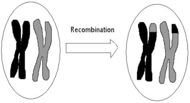
There are various mechanisms for recombination. The most well-known one iscrossing over, where matching regions in homologous chromosomes (which pair during meiosis) experience adouble strand breakand subsequently are reconnected to the other chromosome (see Fig. 2.1). There are other recombination mechanisms like gene conversion, where a stretch of DNA is copied from one chromosome to the matching region of its homologous partner. Exchange of genetic material can also happen in haploid individuals. In this case two different individuals exchange pieces of their genome.

Figure 2.1: Single recombination event by crossing over of chromosomes during meiosis.

The figure shows a pair of homologous chromosomes after the initial duplication, before and after recombination. Black and gray parts derive from different parents. Subsequently, the duplicated pair will segregate into four gametes, two recombined and two not recombined.

2.1 Linkage and linkage disequilibrium

Linkage

Mendel’s second law (of independent assortment) states that genes are inherited indepen- dently of each other. It means that the probability of inheriting a gene at some locus A from one grandmother is independent of whether or not a gene at a different locus B has been inherited from the same grandmother. This “law” is generally only true for gene loci that are located on different chromosomes: they are unlinked. On the other hand, if genes are on the same chromosome, they are said to be physically linked. Linked genes are not inherited independently of each other. In particular, if gene loci are very close to each other, recombination between them is rare and they are typically inherited together.

Mathematically, this is expressed by the recombination fraction r = r_AB between loci A and B, which defines the probability that genes inherited from different grandparents at these loci end up on the same parental gamete (sperm, egg, pollen) that contributes to the offspring genotype,

a₁b₁ a₂b₂

−→













 a₁b₁ a₂b₂

freq. ¹₂(1−r) each a₁b₂

a₂b₁

freq. ¹₂ ·r each

. (2.1)

Here, a₁ and b₁ (res. a₂ and b₂) do not denote an allelic state, but only the origin of the gene either from grandparent 1 or 2.

• r is often also called a recombination rate, but it is really a probability in discrete generation models. We generally have r = 1/2 as upper limit for unlinked loci on different chromosomes and 0≤r <1/2 for linked loci.

• We can define a molecular recombination probability ρas the probability for recom- bination between neighboring base pairs along a chromosome. Typical values are ρ ≈ 10⁻⁸ per generation. However, ρ generally depends strongly on the genomic position x. The estimation of recombination maps ρ(x) from data is an important task of genomics.

• For a given recombination map, we can define a recombination distance d along a chromosome in units of Morgans (named after Thomas Morgan). A distance ofd = 1M indicates that there is on average one recombination breakpoint per generation within the stretch (e.g., due to crossing over). Typical lengths of chromosome regions measure in centi-Morgans(cM).

• The recombination fractionrbetween loci on the same chromosome is the probability of an odd number of recombination breakpoints between these loci. Ignoring interfer- ence of recombination events in neighboring regions, r relates to the recombination