7 Fixed-point logic with counting

(1)

Algorithmic Model Theory SS 2016

Prof. Dr. Erich Grädel and Dr. Wied Pakusa

Mathematische Grundlagen der Informatik

(2)

c b n d

This work is licensed under:

http://creativecommons.org/licenses/by-nc-nd/3.0/de/

Dieses Werk ist lizenziert unter:

http://creativecommons.org/licenses/by-nc-nd/3.0/de/

http://www.logic.rwth-aachen.de

(3)

7 Fixed-point logic with counting

The (machine-independent) characterisation of complexity classes by logics (in the sense of Definition 2.4) yields deep insights into the structure of the classified problems. The theorem of Fagin (cf. Chapter 2) is a seminal result in the field of descriptive complexity theory, and gives such a correspondence between algorithmic and logical resources for the important class NP. If we restrict to ordered structures, we can also find such characterisation for PTIME as shown e.g. in the Immerman-Vardi theorem (cf. Chapter 3). However, it is still one of the major open ques- tions in finite model theory whether there is a logic capturing PTIME onallfinite structures. Note that if no such logic exists this would necessarily imply PTIME̸=∃SO=NP.

As we will see, fixed-point logics, such as LFP or IFP, do not suffice to capture PTIME on arbitrary structures, and most of the naturally considered examples to separate them from PTIME involve some kind of counting. For instance, the simple class EVEN={^A: |A|is even} turns out to be not definable in LFP. Therefore Immerman proposed that counting quantifiers should be added to logics and asked whether a suitable variant of fixed-point logic with counting would suffice to capture PTIME.

Although Cai, Fürer and Immerman eventually answered this ques- tion negatively, the extension of fixed-point logic by counting terms (FPC) has turned out to be an important and robust logic, that defines a natural level of expressiveness. In this chapter we study the logic FPC and present the construction of Cai, Fürer and Immerman which yields the separation of FPC from PTIME. To be precise, we even present a slightly more general result which uses the concept of treewidth and which is due to Dawar and Richerby.

(6)

7 Fixed-point logic with counting

7.1 Logics with Counting Terms

There are different ways of adding counting mechanisms to a logic, which are not necessarily equivalent. The most straightforward pos- sibility is the addition of quantifiers of the form∃^≥2,∃^≥3, etc., with the obvious meaning. While this is perfectly reasonable for bounded- variable fragments of first-order logic or infinitary logic it does not increase the expressiveness of logics such as FO or LFP, since they are closed under the replacement of∃^≥ⁱbyiexistential quantifiers. For fixed-point logic another severe restriction is that it does not allow for recursion over the counting parametersiin quantifiers∃^≥ix. These counting parameters should therefore be considered as variables that range over natural numbers. To define in a precise way a logic with counting and recursion, one extends the original objects of study, namely finite (one-sorted) structuresA, to two-sorted auxiliary structuresA^∗ with a second numerical (but also finite) sort.

Definition 7.1.With any one-sorted finite structureAwith universeA, we associate the two-sorted structureA^∗:=A∪ ⟨{˙ 0, . . . ,|A|};≤, 0,e⟩, where≤is the canonical ordering on{0, . . . ,|A|}, and 0 andestand for the first and the last element. Thus,A^∗is the disjoint union ofAwith a linear order of length|A|+1.

For all logics we studied so far, we naturally obtain two-sorted variants definining properties of the extended structuresA^∗. For instance, formulas of two-sorted first-order logic over two-sorted vocabularies σ∪ {≤, 0,e}are evaluated in structuresA^∗where semantics are defined in the obvious way. From now on, we stick to the convention to use Latin lettersx,y,z, . . . for the variables over the first sort, and Greek lettersλ,µ,ν, . . . for variables over the second sort (the numerical sort).

In counting logics, these two sorts are related bycounting terms, defined by the following rule. Letφ(x)be a formula with a variablex(over the first sort) among its free variables. Then #x[φ]is a term in the second sort, with the set of free variables free(#x[φ]) =free(φ)− {x}. The value of #x[φ]is the number of elementsathat satisfyφ(a).

We introduce counting logics starting with first-order logic with counting, denoted by FOC, which is the closure of two-sorted first-order

106

(7)

7.2 Fixed-Point Logic with Counting logic under counting terms. Here are two simple examples that illustrate the use of counting terms.

Example 7.2. On an undirected graph G = (V,E), the formula

∀x∀y(#z[Exz] =#z[Eyz])expresses the assertion that every node has the same degree, i.e., thatGis regular.

Example7.3. We present below a formulaψ(E1,E2)∈FOC which expresses the assertion that two equivalence relationsE₁andE₂are iso- morphic; of course a necessary and sufficient condition for this is that for everyi, they have the same number of elements in equivalence classes of sizei:

ψ(E1,E2)≡(∀µ)(#x[#y[E1xy] =µ] =#x[#y[E2xy] =µ]).

7.2 Fixed-Point Logic with Counting

We now define(inflationary) fixed point logic with counting (FPC) and partial fixed point logic with countingPFPC by adding to FOC the usual rules for building inflationary or partial fixed points, ranging over both sorts.

Definition 7.4. Inflationary fixed point logic with counting, FPC, is the closure of two-sorted first-order logic under the following rules:

(1) The rule for building counting terms.

(2) The usual rules of first-order logic for building terms and formulae.

(3) The fixed-point formation rule. Suppose thatψ(R,x,µ)is a formula of vocabularyτ∪ {R}wherex=x1, . . . ,xk,µ=µ1, . . . ,µℓ, andR has mixed arity(k,ℓ), and that(u,ν)is ak+ℓ-tuple of first- and second-sort terms, respectively. Then

[ifp Rxµ.ψ](u,ν) is a formula of vocabularyτ.

The semantics of[ifp Rxµ.ψ]onA^∗is defined in the same way as for the logic IFP, namely as the inflationary fixed point of the operator

Fψ:R7−→R∪ {(a,i)|(A^∗,R)|=ψ(a,i)}.

(8)

The definition of PFPC is analogous, where we replace inflationary fixed points by partial ones. In the literature, one also finds different variants of fixed-point logic with counting where the two sorts are related bycounting quantifiersrather than counting terms. Counting quantifiers have the form(∃i x)for ‘there exist at leastidifferentx’, whereiis a second-sort variable. It is obvious that the two definitions are equivalent.

In fact, FPC is a very robust logic. For instance, its expressive power does not change if one permits counting over tuples, even of mixed type, i.e. terms of the form #x,µφ(see exercise class). One can of course also define least fixed-point logic with counting, LFPC, but one has to be careful with the positivity requirement (which is more natural when one uses counting quantifiers rather than counting terms). The equivalence of LFP and IFP readily translates to LFPC≡IFPC.

Example7.5. An interesting example of an FPC-definable query is the method ofstable colourings for graph-canonization. Given a graphG with a colouringf:V→ {0, . . . ,r}of its vertices, we define a refinement f^′off, giving to a vertexxthe new colourf^′x= (f x,n1, . . . ,nr)where n_i=#y[Exy∧(f y=i)]. The new colours can be sorted lexicographically so that they again form an initial subset ofN. Then the process can be iterated until a fixed point, thestable colouring ofGis reached. It is easy to see that the stable colouring of a graph is polynomial-time computable and uniformly definable in FPC.

On many graphs, the stable colouring uniquely identifies each vertex, i.e. no two distinct vertices (i.e. vertices in different orbits of the automorphism group) get the same stable colour. In this way stable colourings provide a polynomial-time graph canonization algorithm for such classes of graphs. For instance, this is the case for the class of all trees or, more generally, any class of graphs with bounded treewidth.

We now discuss the expressive power and evaluation complexity of fixed-point logic with counting. We are mainly interested in FPC- formulae and PFPC-formulae without free variables over the second sort, so that we can compare them with the usual logics without counting.

Exercise 7.1.Even without making use of counting terms, IFP over two- sorted structuresA^∗is more expressive than IFP overA. To prove this, construct a two-sorted IFP-sentenceψsuch thatA^∗|=ψif, and only if,

108

(9)

7.2 Fixed-Point Logic with Counting

|A|is even.

It is clear that counting terms can be computed in polynomial-time.

Hence the data complexity remains in PTIME for FPC and in PSPACE for PFPC. We shall see below that these inclusions are strict.

Theorem 7.6.On finite structures,

(1) IFP⊊FPC⊊PTIME.

(2) PFP⊊PFPC⊊PSPACE.

7.2.1 Infinitary Logic with Counting

LetC_∞ω^k be the infinitary logic withkvariablesL^k_∞ω, extended by the quantifiers ∃^≥m (‘there exist at leastm’) for allm ∈ ^N. Further, let C^ω_∞ω:=^S_kC_∞ω^k .

Proposition 7.7. PFPC⊆C^ω_∞ω.

Due to the two-sorted framework, the proof of this result is a bit more involved than for the corresponding result without counting, but not really difficult (see exercise class).

The separation of FPC from PTIME has been established by Cai, Fürer, and Immerman. Their proof also provides an analysis of the method of stable colourings for graph canonization. We have described this method in its simplest form in Example 7.1. More sophisticated variants compute and refine colourings ofk-tuples of vertices. This is called thek-dimensional Weisfeiler–Lehman methodand, in logical terms, it amounts to labelling eachk-tuple by its type ink+1-variable logic with counting quantifiers. It was conjectured that this method could provide a polynomial-time algorithm for graph isomorphism, at least for graphs of bounded degree. However, Cai, Fürer, and Immerman were able to construct two families(Gn)_n∈Nand(Hn)_n∈Nof graphs such that on one hand,GnandHnhaveO(n)nodes and degree three, and admit a linear-time canonization algorithm, but on the other hand, in first- order (or infinitary) logic with counting,Ω(n)variables are necessary to distinguish betweenGnandHn. In particular, this implies Theorem 7.6.

(10)

7.3 The k-pebble bijection game

In Chapter??we introduced Ehrenfeucht-Fraïssé games to characterize the equivalence of structures (or, to put it in another way, definability of classes) in first-order logic. More specifically, two relational structuresA andBcan be distinguished by an FO-sentence of quantifier-rank≤mif, and only if, Spoiler has a winning strategy in them-move Ehrenfeucht- Fraïssé game played onAandBwhich was denoted byEFm(A,B).

Our next aim is to introduce thek-pebble bijection gamewhich is an extension of the standard Ehrenfeucht-Fraïssé game to capture definability inC_∞ω^ω . We will use these games to show that a certain (polynomial-time decidable) class of graphs is not definable inC_∞ω^ω . In particular, this yields the separation of FPC from PTIME by Proposition 7.7.

Definition 7.8. Thek-pebble bijection game k-BG(A,B) is a two-player game played on relational structures A and B using k pairs of pebbles(x1,y1), . . . ,(xn,yn) that can be placed on pairs of elements (a₁,b₁), . . . ,(an,bn)∈A×Bduring a play. The goal of Player I, who is calledSpoiler, is to show thatA̸≡^C^∞ω^k Bwhile Player II, theDuplicator, claims thatA≡^C^k^∞ωB.

A position in the game k-BG(A,B) is a (partial) assignment (a₁,b₁), . . . ,(an,bn) of pebbles on A×B, so formally, a position is a (partial) mappingp:{1, . . . ,k} →A×B. The initial position isp=∅.

At positionpa play proceeds as follows: First, Spoiler selects a pair of pebblesi≤k. Duplicator has to react with a bijectionh : A→ B which respects all remaining pairs of pebbled elements (except fori), i.e. for alli̸=j∈dom(p)andp(j) = (aj,bj)we haveh(aj) =bj. Spoiler then choosesa∈Aand the position is updated to(p|i7→(ai,bi))where

(p|i7→(ai,bi))(j):=





p(j) j̸=i (a,h(a)) j=i..

Spoiler wins a play, if either|A| ̸=|B|(i.e. Duplicator cannot respond with a bijection), or the play eventually reaches a positionpsuch that the induced mappingp({1, . . . ,k})is not a partial isomorphism ofAandB, i.e. ifp({1, . . . ,k})̸∈Loc(A,B). Infinite plays are won by Duplicator.

110

(11)

7.4 The construction of Cai, Fürer and Immerman

Theorem 7.9.If Duplicator wins the gamek-BG(A,B), thenA≡^C^k^∞ω B.

Proof. We prove by induction that for all formulaeφ(x1, . . . ,xk)∈C^k_∞ω, structuresAandBand alla1, . . . ,a_k∈Aandb1, . . . ,b_k∈Bwe have that ifA|=φ(a₁, . . . ,a_k)andB̸|=φ(a₁, . . . ,a_k)then Spoiler has a winning strategy fork-BG(A,B)starting from positionp(i) = (ai,bi).

The cases of quantifier-free formulae, Boolean connectivities and first-order quantifier follow as in the case of Ehrenfeucht-Fraïssé games (cf. lecture notes of mathematical logic). Hence, we only considerφ=

∃^≥ix_jψ(x1, . . . ,x_k). For this case, a winning strategy for Spoiler can be defined in the following way:

• Spoiler selects the pairj≤k.

• Duplicator reacts with a bijectionh:A→Brespecting the remaining pebbled pairs.

We setX = {a ∈ A : A |= ψ(a1, . . . ,an)}andY = {b ∈ B : B |= ψ(b1, . . . ,bn)}. From the assumption we know that|X| ≥iand|Y|<

i, hence there is an a ∈ X such that h(a) ̸∈ Y. Spoiler selects the elementaand the position is updated to(p|j7→(a_j,b_j)). As we have A|= φ(a1, . . . ,an)andB̸|= φ(b1, . . . ,bj−1,h(a),bj+1, . . . ,bn)the claim

follows by induction. q.e.d.

We can use Theorem 7.9 to show that a classKof finite structures is not definable inC^ω_∞ω. In particular, note thatK ̸∈C^ω_∞ωalso implies thatK ̸∈FPC since we have FPC≤C^ω_∞ω.

Proposition 7.10. Let(A_k)_k≥1and(B_k)_k≥1be two sequences of structures such that for infinitely many kwe haveA_k ∈ K,B_k ̸∈ K and Duplicators winsk-BG(A_k,B_k). ThenKcannot be defined inC^ω_∞ω.

7.4 The construction of Cai, Fürer and Immerman

We now present the construction of Cai, Fürer and Immmerman which yields the separation of FPC from PTIME. Throughout this section, let G= (V,E)denote a connected graph with deg(v) ≥2 for allv∈V.

Starting from Gwe define a family of graphs(X_S(G))_S⊆Ethat result by replacing every vertexvinGby a gadgetZ(v)and interconnecting different gadgets according to the edge relation inG.

(12)

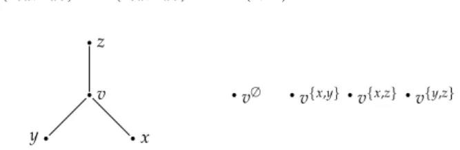
For everyvwe define the set of new verticesZ(v)as

Z(v):={avw,bvw,cvw,dvw:w∈vE} ∪ {v^X:X⊆vE,|X|even}. Vertices of the form avw,bvw are calledouter verticesand they are intended to connect the two gadgetsZ(v)andZ(w). The verticescvw,dvw

arecolour verticeswhich are used only to make the set of outer nodes first-order definable. The remaining verticesv^S are called the inner vertices.

LetX_∅(G)denote the graph over the vertex set^S_v_∈_VZ(v)with the following edges:

•(avw,cvw),(bvw,cvw),(dvw,cvw)for(v,w)∈E,

•(avw,v^X)forw∈X,

•(bvw,v^X)forw̸∈X, and

•(avw,awv)and(bvw,bwv)for all(v,w)∈E.

v y x

z

v^∅ v^{^x,y^} v^{^x,z^} v^{^y,z^}

Figure 7.1.Example: gadget for a vertexvof degree three

In Figure 7.1 the construction of a gadgetZ(v)is illustrated for the case of a vertexvwith degree three. The pairs of outer nodesavx,bvx, avy,bvyandavz,bvzare connected to the corresponding outer nodes of the gadgetsZ(x),Z(y)andZ(z), respectively (this is indicated by the dashed lines in the figure).

We now extend the construction: for any (symmetric) setS⊆ E we defineX_S(G)to be the graphX_∅(G)in which for all(v,w)∈Sthe edges(avw,awv)and(bvw,bwv)are replaced by(avw,bwv)and(awv,bwv). We say that the edges inShave beentwisted. In this way we obtain for every subsetS⊆Eof edges aCFI-graph X_S(G). Interestingly, we are going to show that these CFI-graphsXS(G)are completely determined by the parity of the setS:

112

(13)

7.4 The construction of Cai, Fürer and Immerman

Lemma 7.11.For allS,T⊆Ewe have:

XS(G)∼=XT(G) ⇔ |S| ≡ |T| mod 2.

Before we prove this claim in general, we consider some special cases. First of all, let all twisted edges be incident with a single vertexv.

Lemma 7.12.LetS,T⊆vEbe sets of neighbours of some vertexv∈V.

IfS∆T= (S\T)∪(T\S)is even, then Xv×S(G)∼=Xv×T(G).

Proof. The mappingπ_v;S;T:Xv×S(G)→Xv×T(G)defined by

π_v;S;T(z):=











z, z̸∈Z(v)orzcolour vertex, z, z∈ {avw,bvw},(v,w)∈S∩T, bvw, z=avw,(v,w)∈S∆T, avw, z=bvw,(v,w)∈S∆T, v^X∆(S∆T), z=v^X,

is an isomorphism (use that sinceXandS∆Tare even, the same holds for the symmetric differenceX∆(S∆T)). q.e.d.

We proceed to explain how one obtains an isomorphism between X_{e}(G)andX_{f}(G)for two distinct edgeseand fofG.

Lemma 7.13. X_{e}(G)∼=X_{_f}(G).

Proof. Ifeand f are incident with the same vertex v, then the claim follows by Lemma 7.12. Hence, lete= (u,v)andf = (x,y)be such that {u,v} ∩ {x,y}=∅. Choose a pathv=v1,v2, . . . ,vℓ=xconnectingv andxwithv_i̸∈ {u,y}for alli≥1. Then

π_e_7→_f:=π_v₁_;u;v₂◦π_v₂_;v₁_;v₃◦ · · · ◦π_v_l−1_;v_l−2_;x◦π_v_l_;v_l−1_;y,

is an isomorphism ofX_{_e_}(G)∼= X_{_f_}(G): the twist at edge(u,v) is moved along the path to the twist at edge(x,y)where both twists cancel out each other. Note that along the path, at every inner node viwe

(14)

have precisely two twists of edges for the gadgetZ(v_i)which, again by Lemma 7.12, preserves the structure of the inner nodes. q.e.d.

We are now ready to prove Lemma 7.11.

Proof (of Lemma 7.11). First of all, let|S| ≡ |T| mod 2. If|S|=|T|=1, then the claim follows by Lemma 7.13, so assume that|S| ≥ 2 (or analogously, |T| ≥ 2). Choosee,f ∈ S withe ̸= f. Ife and f are incident with the same vertexv∈Vwe know thatX_S\{e,_f}(G)∼=X_S(G) by Lemma 7.12. In the other case, we use the isomorphismπ_e_7→_fand see thatX_S\{e,_f}(G)∼=XS(G). The claim follows by induction on|S∆T|. For the other direction assume thatπ:X_{f_=(x,y)_}(G)→X∅(G)is an isomorphism. Clearly,πmaps outer (inner, colour) nodes to outer (inner, coulour) nodes, and sinceπalso induces an isomorphism of G, we can assume that for allv ∈ V we haveπ(Z(v)) = Z(v)and π({avw,bvw}) ={avw,bvw}for all(v,w)∈E. At this point we observe that ifπinterchangesavwandbvwit necessarily interchangesawvand bwvfor all edges(v,w)∈Eexcept for(x,y). Hence, the total number of interchanges ofa’s andb’s inπis odd. This contradicts Lemma 7.12, however, as the number of interchanges ofa’s andb’s in πfor each

gadget has to be even. q.e.d.

We conclude that, up to isomorphism, there are precisely two CFI- graphs forGand we fix two canonical representatives from the isomorphism classes:

•X(G):=X∅(G)(theeven CFI-graph for G)

• ˜X(G):=X_{e}(G)for some edgee∈E(theodd CFI-graph for G) TheCFI-queryis to decide, given a CFI-graphXS(G), whetherXS(G)is even or odd, i.e. whetherXS(G)∼=X(G)orXS(G)∼=X^˜(G).

Theorem 7.14.The CFI-query can be decided in polynomial time.

Proof. In order to count the number of twists, we need to identify the aand b-vertices. To this end it suffices to fix in every gadget Z(v) an arbitrary inner node and to associate the intended labeling to the gadgetZ(v)(e.g. declare this node to bev^∅and assign to all connected verticesb-labels and to the remaining outer onesa-labels). Then it is straightforward to count the number of twists modulo two. Lemma 7.11

114

(15)

7.4 The construction of Cai, Fürer and Immerman guarantees that the isomorphism class of the resulting{a,b}-labeled graph is independent of the initial choice of inner vertices. q.e.d.

We conclude that the even and odd CFI-graphs can be distinguished in polynomial time. However, we are going to show that they cannot be separated by sentences inC_∞ω^ω if we start from a class of graphsGwith sufficient complexity. In order to measure the complexity of graphs we introduce the important and well-studied concept oftreewidth. Intuitively the treewidth of a graph formalises to what extent an (undirected) graph resembles a tree, and one of the reasons for its importance is that many NP-hard problems (and even some PSPACE-hard ones) become tractable on classes of graphs with bounded treewidth. There are various equivalent ways to characterize the treewidth of a graph, of which we sketch two: an algebraic and a game theoretic approach.

Definition 7.15. LetG= (V,E)be an undirected graph. Atree decomposition of Gis an undirected treeT = (T,ET)whereTis a family of subsets ofV, i.e.T⊆ P(V)and

(a)^ST=V, and

(b) for all(u,v)∈Ethere is someX∈Tso that{u,v} ⊆X, and (c) for every vertexv∈Vthe set{X∈T:v∈X}is connected inT. Nodes in the treeT are calledbags. Thewidthof the tree decompo- sitionT = (T,ET)is (max{|X|:X∈T} −1), and thetreewidth of G, denoted by tw(G), is defined to be the minimal width for which a tree decomposition ofGexists.

Next, we describe a game which characterises the notion of treewidth. The k-cops and robber gameonGis played by two players, Player I (the cops) and Player II (the robber). The rules are as follows:

the cops possesskpebbles (cops) which they can place on vertices of the graph. The robber has one pebble which is moved along paths. In each move the cops first choose some pebble which is either currently not placed on a vertex of the graph or which is removed from its current positionw. Secondly, the cops determine a vertexvto be the new position for this pebble. After that, the robber reacts by moving his pebble along a path to a new vertex (which may be the old one). The chosen path has to be cop-free where the verticesvandwcount as cop-free for

(16)

the current move. The cops win a play if, and only if, they can reach a position such that the robber cannot move. All other plays, i.e. all infinite ones, are won by the robber.

Seymour proved that a graphGhas treewidthkif, and only if, the cops have a winning strategy in the game withk+1 pebbles, but the robber wins the game if the cops are restricted tokpebbles. We use this game-theoretic characterisation to show:

Theorem 7.16.LetG= (V,E)be a graph withδ(G)≥2 and tw(G)≥k.

Then

X(G)≡^C^∞ω^k X^˜(G).

Proof. For two vertices u,v let σ[u,v] be the permutation which ex- changesu andv and fixes all other points. We say that a bijection h:X(G)→X^˜(G)isgood except at node u∈Vif

•h(Z(v)) =Z(v)for allv∈V,

•hmaps inner vertices to inner vertices and outer vertices to outer vertices,

•his an isomorphism between the subgraphsX(G)\ {v^X:X⊆vE} and ˜X(G)\ {v^X:X⊆vE}, and

• for every pair(auv,buv) ∈Z(u), the mappingh◦σ[auv,buv]is an isomorphism fromX(G)[Z(u)]to ˜X(G)[Z(u)].

Let ˜X(G) =X_(u,v)(G). Then for instanceσ[auv,buv]is good except atuandσ[avu,bvu]is good except atv. Note that ifη∈Aut(X^˜(G))with η(Z(v)) =Z(v)for allv∈Vandhis good except at vertexu, thenh◦η is good except atuas well.

The property of being good at some vertex can be propagated along a path inG: letPbe a simple path inGfromutov, P: u = v₁,v₂, . . . ,v_l−1,v_l=v, and lethbe a bijection which is good except at vertexu. Then the bijectionh^′:=h◦^ηPwhere

η_P:=σ[auv2,buv2]◦πv2;v1;v3◦ · · · ◦π_v_l−1_;v_l−2_;v_o_mel◦σ[avvl−1,bvvl−1], is good except atvand forw̸∈P,x∈Z(w)we haveh^′(x) =h(x).

Finally, we describe a winning strategy for Duplicator in the k-

116

(17)

7.4 The construction of Cai, Fürer and Immerman pebble bijection game played onX(G)and ˜X(G). The strategy satisfies that pairs of pebbles(ai,bi)are always placed on vertices in a common gadget Z(v). First of all, we initialize an instance of thek-cops and robber game played on G where we identify each of the kpairs of pebbles with one of the cops, and we assume that the robber makes his moves according to a fixed winning strategy (recall that tw(G)≥k).

The positions in the two games are related as follows: the vertex inG occupied by thei-th cop is precisely the vertexv ∈V for which the corresponding gadgetZ(v)inX(G)andX(˜G)is pebbled with thei-th pair(a_i,b_i)of pebbles in thek-pebble bijection game. We update the positions in the cops and robber game after each round of thek-pebble bijection game accordingly. Furthermore, whenever the robber is at some vertexv∈V, then Duplicator chooses in her current move some bijection which is good except at vertexv. For convenience, we assume that the robber starts at nodeu, and that in the first round Duplicator answers with the bijectionσ[auv,buv]. Recall that this bijection is good except at vertexu.

We proceed to show that Duplicator can maintain the following invariant during each play: let((a1, . . . ,a_k),(b1, . . . ,b_k))be the current position in thek-pebble bijection game, then

there is a bijectiong:X(G)→X^˜(G)withg(ai) =bifori≤ksuch that gis good except at a vertexu∈Vand fori≤kwe havea_i,b_i̸∈Z(u)(u

is the robber’s position in the cops and robber game).

This can be seen as follows: assume Spoiler chooses thei-th pair of pebbles. Duplicator answers with the bijectiongand Spoiler puts the i-th pair of pebbles onto some tuple(a,g(a)). By the condition ongof being good except atu, the new position in thek-pebble bijection game is indeed a partial isomorphism (gis an isomorphism except at gadget Z(u), and Spoiler would need more than one pebble there to uncover the difference). The move of Spoiler induces an update for theith cop in the cops and robber game, which yields a response of the robber according to his winning strategy, i.e. a move along a cop-free pathPto some vertexv. Hence, as shown above, the bijectiong^′:=g◦ηPrespects all

(18)

pebbled pairs of elements and is good except atv. SinceZ(v)is cop-free (and hence not pebbled), the claim follows. q.e.d.

Theorem 7.17. FPC⊊PTIME on every class of graphs which contains CFI-graphsX(G)and ˜X(G)for graphsGof arbitrary large treewidth.

In fact, Grohe and Marino proved that FPC ≡ PTIME on every class of graphs with bounded treewidth. Their theorem allows us to reformulate the result in a very neat way.

We first observe that the treewidth of X(G) is bounded by (O)(tw(G)): from a tree-decomposition ofGone obtains a tree decomposition ofX(G)by replacing in all bags the vertices by their corresponding gadgets. Furthermore, the size of a gadgetZ(v)inX(G)is bounded by(4∆(G)·2^∆(G)−1)∈ O(∆(G)). Now letGnbe then×ngrid, then tw(Gn) =n,∆(Gn) =4 and

tw(X(G))≤(4∆(G)·2^∆(G)−1)tw(Gn) =24n∈ O(|G|). For a functionf :N→^Nwe define the class of graphs

TW_f:={G: tw(G)≤f(|G|)}.

Theorem 7.18.FPC≡PTIME on TW_f if, and only if,f∈ O(1). Proof. The direction from right to left is mentioned theorem due to Marino and Grohe. For the other direction, assumef̸∈ O(1); then for everyn>0, there existsk> |X(Gn)|with f(k)≥ 24n. Hence, TWf

containsX(Gn)and ˜X(Gn)for everyn≥0. q.e.d.

118

7 Fixed-point logic with counting

Algorithmic Model Theory SS 2016

Prof. Dr. Erich Grädel and Dr. Wied Pakusa

c b n d

Contents

7 Fixed-point logic with counting

7.1 Logics with Counting Terms

7.2 Fixed-Point Logic with Counting

7.3 The k-pebble bijection game

7.4 The construction of Cai, Fürer and Immerman