Logic and Games SS 2009
Prof. Dr. Erich Grädel
Łukasz Kaiser, Tobias Ganzow
Mathematische Grundlagen der Informatik RWTH Aachen
c b n d
This work is licensed under:
http://creativecommons.org/licenses/by-nc-nd/3.0/de/
Dieses Werk ist lizensiert uter:
http://creativecommons.org/licenses/by-nc-nd/3.0/de/
© 2009 Mathematische Grundlagen der Informatik, RWTH Aachen.
http://www.logic.rwth-aachen.de
1 Finite Games and First-Order Logic 1
1.1 Model Checking Games for Modal Logic . . . 1
1.2 Finite Games . . . 4
1.3 Alternating Algorithms . . . 8
1.4 Model Checking Games for First-Order Logic . . . 18
2 Parity Games and Fixed-Point Logics 21 2.1 Parity Games . . . 21
2.2 Fixed-Point Logics . . . 31
2.3 Model Checking Games for Fixed-Point Logics . . . 34
3 Infinite Games 41 3.1 Topology . . . 42
3.2 Gale-Stewart Games . . . 49
3.3 Muller Games and Game Reductions . . . 58
3.4 Complexity . . . 72
4 Basic Concepts of Mathematical Game Theory 79 4.1 Games in Strategic Form . . . 79
4.2 Iterated Elimination of Dominated Strategies . . . 87
4.3 Beliefs and Rationalisability . . . 93
4.4 Games in Extensive Form . . . 96
1 Finite Games and First-Order Logic
An important problem in the field of logics is the question for a given logicL, a structureAand a formulaψ∈ L, whetherAis a model of ψ. In this chapter we will discuss an approach to the solution of this model checking problemvia games for some logics. Our goal is to reduce the problemA |= ψto a strategy problem for amodel checking game G(A,ψ)played by two players calledVerifier(orPlayer0) andFalsifier (orPlayer1). We want to have the following relation between these two problems:
A|=ψ iff Verifier has a winning strategy forG(A,ψ).
We can then do model checking by constructing or proving the existence of winning strategies.
1.1 Model Checking Games for Modal Logic
The first logic to be considered is propositional modal logic (ML). Let us first briefly review its syntax and semantics:
Definition 1.1. For a given set of actions A and atomic properties {Pi:i∈I}, the syntax of ML is inductively defined:
• All propositional logic formulae with propositional variablesPiare in ML.
• Ifψ,ϕ∈ML, then also¬ψ,(ψ∧ϕ)and(ψ∨ϕ)∈ML.
• Ifψ∈ML anda∈A, then⟨a⟩ψand[a]ψ∈ML.
Remark1.2. If there is only one actiona ∈ A, we write ♦ψand ψ instead of⟨a⟩ψand[a]ψ, respectively.
Definition 1.3. Atransition systemorKripke structurewith actions from a setAand atomic properties{Pi:i∈I}is a structure
K= (V,(Ea)a∈A,(Pi)i∈I)
with a universeV of states, binary relationsEa ⊆V×Vdescribing transitions between the states, and unary relationsPi⊆Vdescribing the atomic properties of states.
A transition system can be seen as a labelled graph where the nodes are the states ofK, the unary relations are labels of the states, and the binary transition relations are the labelled edges.
Definition 1.4. Let K = (V,(Ea)a∈A,(Pi)i∈I) be a transition system, ψ∈ML a formula andva state ofK. Themodel relationshipK,v|=ψ, i.e.ψholds at statevofK, is inductively defined:
•K,v|=Piif and only ifv∈Pi.
•K,v|=¬ψif and only ifK,v̸|=ψ.
•K,v|=ψ∨ϕif and only ifK,v|=ψorK,v|=ϕ.
•K,v|=ψ∧ϕif and only ifK,v|=ψandK,v|=ϕ.
•K,v|=⟨a⟩ψif and only if there existswsuch that(v,w)∈Eaand K,w|=ψ.
•K,v|= [a]ψif and only ifK,w|=ψholds for allwwith(v,w)∈Ea. Definition 1.5. For a transition systemKand a formulaψwe define theextension
JψKK :={v:K,v|=ψ}
as the set of states ofKwhereψholds.
Remark1.6. In order to keep the following propositions short and easier to understand, we assume that all modal logic formulae are given in negation normal form, i.e. negations occur only at atoms. This does not change the expressiveness of modal logic as for every formula an equivalent one in negation normal form can be constructed. We omit a proof here, but the transformation can be easily achieved by applying
DeMorgan’s laws and the duality ofand♦(i.e.¬⟨a⟩ψ≡[a]¬ψand
¬[a]ψ≡ ⟨a⟩¬ψ) to shift negations to the atomic subformulae.
We will now describe model checking games for ML. Given a transition systemKand a formulaψ∈ML, we define a gameG that contains positions(ϕ,v)for every subformulaϕofψand everyv∈V.
In this game, starting from position(ϕ,v), Verifier’s goal is to show thatK,v|=ϕ, while Falsifier tries to proveK,v̸|=ϕ.
In the game, Verifier is allowed to move at positions (ϕ∨ϑ,v), where she can choose to move to position(ϕ,v)or(ϑ,v), and at posi- tions(⟨a⟩ϕ,v), where she can move to position(ϕ,w)for aw∈vEa. Analogously, Falsifier can move from(ϕ∧ϑ,v)to(ϕ,v)or(ϑ,v)and from([a]ϕ,v) to(ϕ,w)for aw∈vEa. Finally, there are the terminal positions (Pi,v)and (¬Pi,v), which are won by Verifier ifK,v|= Pi andK,v|=¬Pi, respectively, otherwise they are winning positions for Falsifier.
The intuitive idea of this construction is to let the Verifier make the existential choices. To win from one of her positions, a disjunction or diamond subformula, she either needs to prove that one of the disjuncts is true, or that there exists a successor at which the subformula holds.
Falsifier, on the other hand, in order to win from his positions, can choose a conjunct that is false or, if at a box formula, choose a successor at which the subformula does not hold.
The idea behind this construction is that at disjunctions and dia- monds, Verifier can choose a subformula that is satisfied by the structure or a successor position at which the subformula is satisfied, while at conjunctions and boxes, Falsifier can choose a subformula or position that is not. So it is easy to see that the following lemma holds.
Lemma 1.7. LetKbe a Kripke structure,v∈Vandϕa formula in ML.
Then we have
K,v|=ϕ ⇔ Verifier has a winning strategy from(ϕ,v). To assess the efficiency of games as a solution for model checking problems, we have to consider the complexity of the resulting model checking games based on the following criteria:
1.2 Finite Games
• Are all plays necessarily finite?
• If not, what are the winning conditions for infinite plays?
• Do the players always have perfect information?
• What is the structural complexity of the game graphs?
• How does the size of the graph depend on different parameters of the input structure and the formula?
For first-order logic (FO) and modal logic (ML) we have only finite plays with positional winning conditions, and, as we will see, the winning regions are computable in linear time with respect to the size of the game graph (for finite structures of course).
Model checking games for fixed-point logics however admit infinite plays, and we use so calledparity conditionsto determine the winner of such plays. It is still an open question whether winning regions and winning strategies in parity games are computable in polynomial time.
1.2 Finite Games
In the following section we want to deal with two-player games with perfect information and positional winning conditions, given by agame graph(orarena)
G= (V,E)
where the setVof positions is partitioned into sets of positions V0 andV1belonging to Player 0 and Player 1, respectively. Player 0, also calledEgo, moves from positionsv∈V0, while Player 1, calledAlter, moves from positionsv∈V1. All moves are along edges, and we use the termplayto describe a (finite or infinite) sequencev0v1v2. . . with (vi,vi+1)∈Efor alli. We use a simple positional winning condition:
Move or lose! Playerσwins at positionvifv∈V1−σandvE=∅, i.e., if the position belongs to his opponent and there are no moves possible from that position. Note that this winning condition only applies to finite plays, infinite plays are considered to be a draw.
1 Finite Games and First-Order Logic
We define astrategy(for Playerσ) as a mapping f :{v∈Vσ:vE̸=∅} →V
with(v,f(v))∈Efor allv∈V. We call f winningfrom positionvif Playerσwins all plays that start atvand are consistent with f.
We now can definewinning regions W0andW1:
Wσ={v∈V: Playerσhas a winning strategy from positionv}. This proposes several algorithmic problems for a given game G: The computation of winning regionsW0andW1, the computation of winning strategies, and the associated decision problem
Game:={(G,v): Player 0 has a winning strategy forG fromv}. Theorem 1.8. Gameis P-complete and decidable in time O(|V|+|E|).
Note that this remains true forstrictly alternating games.
A simple polynomial-time approach to solve Gameis to compute the winning regions inductively:Wσ=Sn∈NWσn, where
Wσ0={v∈V1−σ:vE=∅}
is the set of terminal positions which are winning for Playerσ, and Wσn+1={v∈Vσ:vE∩Wσn̸=∅} ∪ {v∈V1−σ:vE⊆Wσn} is the set of positions from which Playerσcan win in at mostn+1 moves.
Aftern≤ |V|steps, we have thatWσn+1 =Wσn, and we can stop the computation here.
To solve Gamein linear time, we have to use the slightly more involved Algorithm 1.1. Procedure Propagate will be called once for every edge in the game graph, so the running time of this algorithm is linear with respect to the number of edges inG.
Furthermore, we can show that the decision problem Game is equivalent to the satisfiability problem for propositional Horn formulae.
Algorithm 1.1.A linear time algorithm for Game Input: A gameG= (V,V0,V1,E)
output: Winning regionsW0andW1
for allv∈Vdo (∗1: Initialisation∗) win[v]:=⊥
P[v]:=∅ n[v]:=0 end do
for all(u,v)∈Edo (∗2: CalculatePandn∗) P[v]:=P[v]∪ {u}
n[u]:=n[u] +1 end do
for allv∈V0 (∗3: Calculate win∗) ifn[v] =0thenPropagate(v, 1)
for allv∈V\V0
ifn[v] =0thenPropagate(v, 0) returnwin
procedurePropagate(v,σ) ifwin[v]̸=⊥then return
win[v]:=σ (∗4: Markvas winning for playerσ∗) for allu∈P[v]do (∗5: Propagate change to predecessors∗)
n[u]:=n[u]−1
ifu∈Vσorn[u] =0thenPropagate(u,σ) end do
end
We recall that propositional Horn formulae are finite conjunctions Vi∈ICiof clausesCiof the form
X1∧. . .∧Xn → X or X1∧. . .∧Xn
| {z }
body(Ci)
→ |{z}0
head(Ci)
.
A clause of the formXor 1→Xhas an empty body.
We will show that Sat-Hornand Game are mutually reducible via logspace and linear-time reductions.
(1) Game≤log-linSat-Horn
For a game G = (V,V0,V1,E), we construct a Horn formulaψG with clauses
v→u for allu∈V0and(u,v)∈E, and v1∧. . .∧vm→u for allu∈V1anduE={v1, . . . ,vm}. The minimal model of ψG is precisely the winning region of Player 0, so
(G,v)∈Game ⇐⇒ ψG∧(v→0)is unsatisfiable.
(2) Sat-Horn≤log-linGame
For a Horn formulaψ(X1, . . . ,Xn) =Vi∈ICi, we define a game Gψ= (V,V0,V1,E)as follows:
V={|0} ∪ {X{z1, . . . ,Xn}}
V0
∪ {|Ci:{zi∈I}}
V1
and
E={Xj→Ci:Xj=head(Ci)} ∪ {Ci→Xj:Xj∈body(Ci)}, i.e., Player 0 moves from a variable to some clause containing the variable as its head, and Player 1 moves from a clause to some variable in its body. Player 0 wins a play if, and only if, the play reaches a clauseCwith body(C) =∅. Furthermore, Player 0 has a winning strategy from positionXif, and only if,ψ|=X, so we
1.3 Alternating Algorithms
have
Player 0 wins from position 0 ⇐⇒ ψis unsatisfiable.
These reductions show that Sat-Hornis also P-complete and, in particular, also decidable in linear time.
1.3 Alternating Algorithms
Alternating algorithms are algorithms whose set of configurations is divided intoaccepting,rejecting,existentialanduniversalconfigurations.
The acceptance condition of an alternating algorithmAis defined by a game played by two players∃and∀on the computation treeTA,x ofAon inputx. The positions in this game are the configurations of A, and we allow movesC →C′ from a configurationCto any of its successor configurationsC′. Player∃moves at existential configurations and wins at accepting configurations, while Player∀moves at universal configurations and wins at rejecting configurations. By definition, A accepts some inputxif and only if Player∃has a winning strategy for the game played onTA,x.
We will introduce the concept of alternating algorithms formally, using the model of a Turing machine, and we prove certain relation- ships between the resulting alternating complexity classes and usual deterministic complexity classes.
1.3.1 Turing Machines
The notion of an alternating Turing machine extends the usual model of a (deterministic) Turing machine which we introduce first. We consider Turing machines with a separate input tape and multiple linear work tapes which are divided into basic units, called cells or fields. Informally, the Turing machine has a reading head on the input tape and a combined reading and writing head on each of its work tapes.
Each of the heads is at one particular cell of the corresponding tape during each point of a computation. Moreover, the Turing machine is in a certain state. Depending on this state and the symbols the machine
1 Finite Games and First-Order Logic is currently reading on the input and work tapes, it manipulates the current fields of the work tapes, moves its heads and changes to a new state.
Formally, a(deterministic) Turing machine with separate input tape and k linear work tapesis given by a tupleM= (Q,Γ,Σ,q0,Facc,Frej,δ), where Q is a finite set of states, Σ is the work alphabet containing a designated symbol (blank), Γ is the input alphabet, q0 ∈ Q is the initial state, F := Facc∪Frej ⊆ Q is the set offinal states (with Facc the accepting states, Frej the rejecting statesand Facc∩Frej = ∅), and δ:(Q\F)×Γ×Σk→Q× {−1, 0, 1} ×Σk× {−1, 0, 1}kis thetransition function.
AconfigurationofMis a complete description of all relevant facts about the machine at some point during a computation, so it is a tuple C= (q,w1, . . . ,wk,x,p0,p1, . . . ,pk)∈Q×(Σ∗)k×Γ∗×Nk+1 whereq is the recent state,wiis the contents of work tape numberi, xis the contents of the input tape,p0is the position on the input tape andpiis the position on work tape numberi. The contents of each of the tapes is represented as a finite word over the corresponding alphabet[, i.e., a finite sequence of symbols from the alphabet]. The contents of each of the fields with numbersj>|wi|on work tape numberiis the blank symbol (we think of the tape as being infinite). A configuration wherex is omitted is called apartial configuration. The configurationCis called finalifq∈F. It is calledacceptingifq∈Faccandrejectingifq∈Frej.
Thesuccessor configurationofCis determined by the recent state and thek+1 symbols on the recent cells of the tapes, using the transition function: Ifδ(q,xp0,(w1)p1, . . . ,(wk)pk) = (q′,m0,a1, . . . ,ak,m1, . . . ,mk,b), then the successor configuration ofCis∆(C) = (q′,w′,p′,x), where for anyi,w′iis obtained fromwiby replacing symbol numberpibyaiand p′i=pi+mi. We writeC⊢MC′if, and only if,C′=∆(C).
Theinitial configuration C0(x) =C0(M,x)ofMon inputx∈Γ∗is given by the initial stateq0, the blank-padded memory, i.e.,wi=εand pi=0 for anyi≥1,p0=0, and the contentsxon the input tape.
AcomputationofMon inputxis a sequenceC0,C1, . . . of config- urations of M, such thatC0 = C0(x) andCi ⊢M Ci+1 for alli ≥ 0.
The computation is calledcompleteif it is infinite or ends in some final
configuration. A complete finite computation is calledacceptingif the last configuration is accepting, and the computation is calledrejecting if the last configuration is rejecting. M acceptsinputxif the (unique) complete computation ofMonxis finite and accepting. M rejectsinput xif the (unique) complete computation ofMonxis finite and rejecting.
The machineM decidesa languageL⊆Γ∗ifMaccepts allx∈ Land rejects allx∈Γ∗\L.
1.3.2 Alternating Turing Machines
Now we shall extend deterministic Turing machines to nondeterministic Turing machines from which the concept of alternating Turing machines is obtained in a very natural way, given our game theoretical framework.
Anondeterministic Turing machineis nondeterministic in the sense that a given configurationCmay have several possible successor config- urations instead of at most one. Intuitively, this can be described as the ability toguess. This is formalised by replacing the transition function δ:(Q\F)×Γ×Σk→Q× {−1, 0, 1} ×Σk× {−1, 0, 1}kby a transition relation∆⊆((Q\F)×Γ×Σk)×(Q× {−1, 0, 1} ×Σk× {−1, 0, 1}k). The notion of successor configurations is defined as in the deterministic case, except that the successor configuration of a configurationCmay not be uniquely determined. Computations and all related notions carry over from deterministic machines in the obvious way. However, on a fixed inputx, a nondeterministic machine now has several possi- ble computations, which form a (possibly infinite) finitely branching computation treeTM,x. A nondeterministic Turing machineM accepts an inputxif thereexistsa computation ofMonxwhich is accepting, i.e., if there exists a path from the rootC0(x)ofTM,xto some accepting configuration. The language of MisL(M) ={x∈Γ∗| Macceptsx}. Notice that for a nondeterministic machine Mto decide a language L⊆Γ∗it is not necessary, that all computations of Mare finite. (In a sense, we count infinite computations as rejecting.)
From a game-theoretical perspective, the computation of a non- deterministic machine can be viewed as a solitaire game on the com- putation tree in which the only player (the machine) chooses a path
through the tree starting from the initial configuration. The player wins the game (and hence, the machine accepts its input) if the chosen path finally reaches an accepting configuration.
An obvious generalisation of this game is to turn it into a two- player game by assigning the nodes to the two players who are called∃ and∀, following the intuition that Player∃tries to show the existence of agoodpath, whereas Player∀tries to show that all selected paths arebad. As before, Player∃wins a play of the resulting game if, and only if, the play is finite and ends in an accepting leaf of the game tree.
Hence, we call a computation tree accepting if, and only if, Player∃has a winning strategy for this game.
It is important to note that the partition of the nodes in the tree should not depend on the inputxbut is supposed to be inherent to the machine. Actually, it is even independent of the contents of the work tapes, and thus, whether a configuration belongs to Player∃or to Player∀merely depends on the current state.
Formally, analternating Turing machineis a nondeterministic Turing machineM = (Q,Γ,Σ,q0,Facc,Frej,∆) whose set of statesQ = Q∃∪ Q∀∪Facc∪Frejis partitioned intoexistential, universal, accepting, and rejectingstates. The semantics of these machines is given by means of the game described above.
Now, if we let accepting configurations belong to player ∀and rejecting configurations belong to player ∃, then we have the usual winning condition that a player loses if it is his turn but he cannot move.
We can solve such games by determining the winner at leaf nodes and propagating the winner successively to parent nodes. If at some node, the winner at all of its child nodes is determined, the winner at this node can be determined as well. This method is sometimes referred to as backwards induction and it basically coincides with our method for solving Gameon trees (with possibly infinite plays). This gives the following equivalent semantics of alternating Turing machines:
The subtreeTCof the computation tree ofMonxwith rootCis calledaccepting, if
•Cis accepting
1.3 Alternating Algorithms
•Cis existential and there is a successor configurationC′ofCsuch thatTC′is accepting or
•Cis universal andTC′ is accepting for all successor configurations C′ofC.
Maccepts an inputx, ifTC0(x)=TM,xis accepting.
For functionsT,S:N→N, an alternating Turing machineMis calledT-time boundedif, and only if, for any inputx, each computation of Mon xhas length less or equal T(|x|). The machine is calledS- space boundedif, and only if, for any inputx, during any computation of Mon x, at most S(|x|) cells of the work tapes are used. Notice that time boundedness implies finiteness of all computations which is not the case for space boundedness. The same definitions apply for deterministic and nondeterministic Turing machines as well since these are just special cases of alternating Turing machines. These notions of resource bounds induce the complexity classes Atimecontaining precisely those languages L such that there is an alternating T-time bounded Turing machine decidingLand Aspacecontaining precisely those languages Lsuch that there is an alternatingS-space bounded Turing machine decidingL. Similarly, these classes can be defined for nondeterministic and deterministic Turing machines.
We are especially interested in the following alternating complexity classes:
• ALogspace=Sd∈NAspace(d·logn),
• APtime=Sd∈NAtime(nd),
• APspace=Sd∈NAspace(nd).
Observe that Game∈Alogspace. An alternating algorithm which decides Gamewith logarithmic space just plays the game. The algo- rithm only has to store thecurrentposition in memory, and this can be done with logarithmic space. We shall now consider a slightly more involved example.
Example1.9. QBF ∈ Atime(O(n)). W.l.o.g we assume that negation appears only at literals. We describe an alternating procedureEval(ϕ,I) which computes, given a quantified Boolean formulaψand a valuation I: free(ψ)→ {0, 1}of the free variables ofψ, the valueJψKI.
1 Finite Games and First-Order Logic Algorithm 1.2.Alternating algorithm deciding QBF.
Input:(ψ,I) whereψ∈QAL andI: free(ψ)→ {0, 1} ifψ=Y then
ifI(Y) =1thenaccept elsereject
ifψ=ϕ1∨ϕ2 then„∃“ guessesi∈ {1, 2},Eval(ϕi,I) ifψ=ϕ1∧ϕ2 then„∀“ choosesi∈ {1, 2},Eval(ϕi,I) ifψ=∃Xϕ then„∃“ guessesj∈ {0, 1},Eval(ϕ,I[X=j]) ifψ=∀Xϕ then„∀“ choosesj∈ {0, 1},Eval(ϕ,I[X=j])
The main results we want to establish in this section concern the relationship between alternating complexity classes and determinis- tic complexity classes. We will see that alternating time corresponds to deterministic space, while by translating deterministic time into alternating space, we can reduce the complexity by one exponential.
Here, we consider the special case of alternating polynomial time and polynomial space. We should mention, however, that these results can be generalised to arbitrary large complexity bounds which are well behaved in a certain sense.
Lemma 1.10. NPspace⊆APtime.
Proof. Let L ∈ NPspace and let M be a nondeterministic nl-space bounded Turing machine which recognisesL for somel ∈ N. The machineMaccepts some inputxif, and only if, some accepting config- uration is reachable from the initial configurationC0(x)in the configu- ration tree ofMonxin at mostk:=2cnlsteps for somec∈N. This is due to the fact that there are mostkdifferent configurations ofMon inputxwhich use at mostnlcells of the memory which can be seen using a simple combinatorial argument. So if there is some accepting configuration reachable from the initial configurationC0(x), then there is some accepting configuration reachable fromC0(x)in at mostksteps.
This is equivalent to the existence of some intermediate configuration C′ that is reachable fromC0(x)in at mostk/2steps and from which some accepting configuration is reachable in at mostk/2steps.
So the alternating algorithm decidingLproceeds as follows. The existential player guesses such a configuration C′ and the universal player chooses whether to check thatC′is reachable fromC0(x)in at mostk/2steps or whether to check that some accepting configuration is reachable fromC′in at mostk/2steps. Then the algorithm (or equiva- lently, the game) proceeds with the subproblem chosen by the universal player, and continues in this binary search like fashion. Obviously, the number of steps which have to be performed by this procedure to decide whether xis accepted by Mis logarithmic ink. Sincekis exponential innl, the time bound ofMisdnl for somed∈N, so M
decidesLin polynomial time. q.e.d.
Lemma 1.11. APtime⊆Pspace.
Proof. Let L ∈APtimeand let Abe an alternating nl-time bounded Turing machine that decidesL for somel ∈ N. Then there is some r∈Nsuch that any configuration ofAon any inputxhas at mostr successor configurations and w.l.o.g. we can assume that any non-final configuration has preciselyrsuccessor configurations. We can think of the successor configurations of some non-final configurationCas being enumerated asC1, . . . ,Cr. Clearly, for givenCandiwe can computeCi. The idea for a deterministic Turing machineMto check whether some inputxis inLis to perform a depth-first search on the computation tree TA,x of A on x. The crucial point is, that we cannot construct and keep the whole configuration treeTA,xin memory since its size is exponential in|x|which exceeds our desired space bound. However, since the length of each computation is polynomially bounded, it is possible to keep a single computation path in memory and to construct the successor configurations of the configuration under consideration on the fly.
Roughly, the procedureMcan be described as follows. We start with the initial configurationC0(x). Given any configurationCunder consideration, we propagate 0 to the predecessor configuration ifCis rejecting and we propagate 1 to the predecessor configuration ifCis accepting. If Cis neither accepting nor rejecting, then we construct,
fori=1, . . . ,rthe successor configurationCiofCand proceed with checkingCi. IfCis existential, then as soon as we receive 1 for somei, we propagate 1 to the predecessor. If we encounter 0 for alli, then we propagate 0. Analogously, ifCis universal, then as soon as we receive a 0 for somei, we propagate 0. If we receive only 1 for alli, then we propagate 1. Thenxis inLif, and only if, we finally receive 1 atC0(x). Now, at any point during such a computation we have to store at most one complete computation ofAonx. SinceAisnl-time bounded, each such computation has length at mostnland each configuration has size at mostc·nlfor somec∈N. SoMneeds at mostc·n2lmemory cells
which is polynomial inn. q.e.d.
So we obtain the following result.
Theorem 1.12. (Parallel time complexity = sequential space complexity) (1) APtime=Pspace.
(2) AExptime=Expspace.
Proposition (2) of this theorem is proved exactly the same way as we have done it for proposition (1). Now we prove that by translating sequentialtimeinto alternatingspace, we can reduce the complexity by one exponential.
Lemma 1.13. Exptime⊆APspace
Proof. LetL∈Exptime. Using a standard argument from complexity theory, there is a deterministic Turing machineM= (Q,Σ,q0,δ)with time boundm:=2c·nk for somec,k∈Nwith only a single tape (serving as both input and work tape) which decides L. (The time bound of the machine with only a single tape is quadratic in that of the original machine withkwork tapes and a separate input tape, which, however, does not matter in the case of an exponential time bound.) Now if Γ=Σ⊎(Q×Σ)⊎ {#}, then we can describe each configurationCof Mby a word
C=#w0. . .wi−1(qwi)wi+1. . .wt#∈Γ∗.
1.3 Alternating Algorithms
SinceMhas time boundmand only one single tape, it has space bound m. So, w.l.o.g., we can assume that|C|=m+2 for all configurations C of Mon inputs of length n. (We just use a representation of the tape which has a priori the maximum length that will occur during a computation on an input of lengthn.) Now the crucial point in the argumentation is the following. If C ⊢ C′ and 1≤ i ≤ m, symbol numberiof the wordC′ only depends on the symbols numberi−1, iandi+1 ofC. This allows us, to decide whetherx∈L(M)with the following alternating procedure which uses only polynomial space.
Player∃guesses some numbers≤mof steps of which he claims that it is precisely the length of the computation of M on input x.
Furthermore, ∃ guesses some state q ∈ Facc, a Symbol a ∈ Σ and a number i ∈ {0, . . . ,s}, and he claims that the i-th symbol of the configurationCofMafter the computation onxis(qa). (So players start inspecting the computation ofMonxfrom the final configuration.) IfMaccepts inputx, then obviously player∃has a possibility to choose all these objects such that his claims can be validated. Player∀wants to disprove the claims of∃. Now, player∃guesses symbolsa−1,a0,a1∈Γ of which he claims that these are the symbols number i−1, i and i+1 of the predecessor configuration of the final configuration C.
Now,∀can choose any of these symbols and demand, that∃validates his claim for this particular symbol. This symbol is now the symbol under consideration, whileiis updated according to the movement of the (unique) head of M. Now, these actions of the players take place for each of the s computation steps of M on x. After s such steps, we check whether the recent symbol and the recent position are consistent with the initial configurationC0(x). The only information that has to be stored in the memory is the positionion the tape, the numberswhich∃has initially guessed and the current number of steps.
Therefore, the algorithm uses space at most O(log(m)) =O(nk)which is polynomial inn. Moreover, ifMaccepts inputxthen obviously, player
∃has a winning strategy for the computation game. If, conversely,M rejects inputx, then the combination of all claims of player∃cannot be consistent and player∀has a strategy to spoil any (cheating) strategy of player ∃by choosing the appropriate symbol at the appropriate
1 Finite Games and First-Order Logic
computation step. q.e.d.
Finally, we make the simple observation that it is not possible to gain more than one exponential when translating from sequential time to alternating space. (Notice that Exptimeis a proper subclass of 2Exptime.)
Lemma 1.14. APspace⊆Exptime
Proof. LetL∈APspace, and letAbe an alternatingnk-space bounded Turing machine which decides L for somek ∈ N. Moreover, for an inputx of A, let Conf(A,x)be the set of all configurations of Aon inputx. Due to the polynomial space bound of A, this set is finite and its size is at most exponential in |x|. So we can construct the graph G = (Conf(A,x),⊢) in time exponential in|x|. Moreover, a configuration C is reachable fromC0(x) in TA,x if and only if C is reachable fromC0(x)inG. So to check whetherAaccepts inputxwe simply decide whether player∃has a winning strategy for the game played onGfromC0(x). This can be done in time linear in the size of G, so altogether we can decide whetherx∈L(A)in time exponential
in|x|. q.e.d.
Theorem 1.15. (Translating sequential time into alternating space) (1) ALogspace=P.
(2) APspace=Exptime.
Proposition (1) of this theorem is proved using exactly the same arguments as we have used for proving proposition (2). An overview over the relationship between deterministic and alternating complexity classes is given in Figure 1.1.
Logspace ⊆ Ptime ⊆ Pspace ⊆ Exptime ⊆ Expspace
|| || || ||
ALogspace ⊆ APtime ⊆ APspace ⊆ AExptime Figure 1.1.Relation between deterministic and alternating complexity classes
1.4 Model Checking Games for First-Order Logic
Let us first recall the syntax of FO formulae on relational structures.
We have thatRi(x¯),¬Ri(x¯),x=yandx̸=yare well-formed valid FO formulae, and inductively for FO formulaeϕandψ, we have thatϕ∨ψ, ϕ∧ψ,∃xϕand∀xϕare well-formed FO formulae. This way, we allow only formulae innegation normal formwhere negations occur only at atomic subformulae and all junctions except∨and∧are eliminated.
These constraints do not limit the expressiveness of the logic, but the resulting games are easier to handle.
For a structureA= (A,R1, . . . ,Rm)withRi ⊆Ari, we define the evaluation gameG(A,ψ)as follows:
We have positionsϕ(a¯)for every subformulaϕ(x¯)ofψand every
¯ a∈Ak.
At a positionϕ∨ϑ, Verifier can choose to move either toϕor to ϑ, while at positions∃xϕ(x, ¯b), he can choose an instantiationa∈Aof xand move toϕ(a, ¯b). Analogously, Falsifier can move from positions ϕ∧ϑ to either ϕorϑand from positions ∀xϕ(x, ¯b)to ϕ(a, ¯b) for an a∈A.
The winning condition is evaluated at positions with atomic or negated atomic formulaeϕ, and we define that Verifier wins atϕ(a¯)if, and only if,A|=ϕ(a¯), and Falsifier wins if, and only if,A̸|=ϕ(a¯).
In order to determine the complexity of FO model checking, we have to consider the process of determining whetherA|=ψ. To decide this question, we have to construct the gameG(A,ψ)and check whether Verifier has a winning strategy from positionψ. The size of the game graph is bound by |G(A,ψ)| ≤ |ψ| · |A|width(ψ), where width(ψ) is the maximal number of free variables in the subformulae of ψ. So the game graph can be exponential, and therefore we can get only exponential time complexity for Game. In particular, we have the following complexities for the general case:
• alternating time:O(|ψ|+qd(ψ)log|A|) where qd(ψ)is the quantifier-depth ofψ,
• alternating space:O(width(ψ)·log|A|+log|ψ|),
• deterministic time:O(|ψ| · |A|width(ψ))and
• deterministic space:O(|ψ|+qd(ψ)log|A|).
Efficient implementations of model checking algorithms will con- struct the game graph on the fly while solving the game.
There are several possibilities of how to reason about the complex- ity of FO model checking. We can consider thestructural complexity, i.e., we fix a formula and measure the complexity of the model checking algorithm in terms of the size of the structure only. On the other hand, theexpression complexitymeasures the complexity in terms of the size of a given formula while the structure is considered to be fixed. Finally, thecombined complexityis determined by considering both, the formula and the structure, as input parameters.
We obtain that the structural complexity of FO model checking is ALogtime, and both the expression complexity and the combined complexity is PSpace.
1.4.1 Fragments ofFOwith Efficient Model Checking
We have just seen that in the general case the complexity of FO model checking is exponential with respect to the width of the formula. In this section, we will see that some restrictions made to the underlying logic will also reduce the complexity of the associated model checking problem.
We will start by considering thek-variable fragment ofFO : FOk:={ψ∈FO : width(ψ)≤k}.
In this fragment, we have an upper bound for the width of the formulae, and we get polynomial time complexity:
ModCheck(FOk)is P-complete and solvable in timeO(|ψ| · |A|k). There are other fragments of FO that have model checking com- plexityO(|ψ| · ∥A∥):
• ML: propositional modal logic,
• FO2: formulae of width two,
• GF: the guarded fragment of first-order logic.
We will have a closer look at the last one, GF.
1.4 Model Checking Games for First-Order Logic
GF is a fragment of first-order logic which allows only guarded quantification
∃y¯(α(x, ¯¯ y)∧ϕ(x, ¯¯ y))and∀y¯(α(x, ¯¯ y)→ϕ(x, ¯¯ y))
where theguardsαare atomic formulae containing all free variables ofϕ.
GF is a generalisation of modal logics, and we have that ML⊆ GF⊆FO. In particular, the modal logic quantifiers♦andcan be expressed as
⟨a⟩ϕ≡ ∃y(Eaxy∧ϕ(y))and[a]ϕ≡ ∀y(Eaxy→ϕ(y)).
Since guarded logics have small model checking games of size
∥G(A,ψ)∥=O(|ψ| · ∥A∥), there exist efficient game-based model check- ing algorithms for them.
2 Parity Games and Fixed-Point Logics
2.1 Parity Games
In the previous section we presented model checking games for first- order logic and modal logic. These games admit only finite plays and their winning conditions are specified just by sets of positions. Winning regions in these games can be computed in linear time with respect to the size of the game graph.
However, in many computer science applications, more expressive logics like temporal logics, dynamic logics, fixed-point logics and others are needed. Model checking games for these logics admit infinite plays and their winning conditions must be specified in a more elaborate way.
As a consequence, we have to consider the theory of infinite games.
For fixed-point logics, such as LFP or the modalµ-calculus, the appropriate evaluation games are parity games. These are games of possibly infinite duration where to each position a natural number is assigned. This number is called thepriorityof the position, and the winner of an infinite play is determined according to whether the least priority seen infinitely often during the play is even or odd.
Definition 2.1. We describe a parity gameby a labelled graph G = (V,V0,V1,E,Ω)where(V,V0,V1,E)is a game graph andΩ:V→N, with |Ω(V)|finite, assigns apriorityto each position. The set V of positions may be finite or infinite, but the number of different priorities, called theindexofG, must be finite. Recall that a finite play of a game is lost by the player who gets stuck, i.e. cannot move. For infinite plays v0v1v2. . ., we have a special winning condition: If the least number appearing infinitely often in the sequenceΩ(v0)Ω(v1). . . of priorities is even, then Player 0 wins the play, otherwise Player 1 wins.
Definition 2.2. A strategy (for Playerσ) is a function f:V∗Vσ→V
such that f(v0v1. . .vn)∈vnE.
We say that a playπ=v0v1. . . isconsistentwith the strategyf of Playerσif for eachvi∈Vσit holds thatvi+1=f(vi). The strategy fis winningfor Playerσfrom (or on) a setW⊆Vif each play starting in Wthat is consistent withf is winning for Playerσ.
In general, a strategy depends on the whole history of the game.
However, in this chapter, we are interested in simple strategies that depend only on the current position.
Definition 2.3. A strategy (of Playerσ) is calledpositional(ormemoryless) if it only depends on the current position, but not on the history of the game, i.e. f(hv) = f(h′v)for allh,h′∈V∗,v∈V. We often view positional strategies simply as functions f : V→V.
We will see that such positional strategies suffice to solve parity games by proving the following theorem.
Theorem 2.4(Forgetful Determinacy). In any parity game, the set of positions can be partitioned into two setsW0andW1such that Player 0 has a positional strategy that is winning on W0 and Player 1 has a positional strategy that is winning onW1.
Before proving the theorem, we give two general examples of positional strategies, namely attractor and trap strategies, and show how positional winning strategies on parts of the game graph may be combined to positional winning strategies on larger regions.
Remark2.5. Let f and f′be positional strategies for Playerσthat are winning on the setsW,W′, respectively. Let f+f′ be the positional strategy defined by
(f+f′)(x):=
f(x) ifx∈W f′(x) otherwise.
Then f+f′is a winning strategy onW∪W′.
Definition 2.6. LetG = (V,V0,V1,E)be a game andX⊆V. We define theattractor of X for Playerσas
Attrσ(X) ={v∈V: Playerσhas a (w.l.o.g. positional) strategy to reach some positionx∈X∪Tσ
in finitely many steps} whereTσ={v∈V1−σ:vE=∅}denotes the set of terminal positions in which Playerσhas won.
A setX⊆Vis called atrapfor Playerσif Player 1−σhas a (w.l.o.g.
positional) strategy that avoids leavingXfrom everyx∈X.
We can now turn to the proof of the Forgetful Determinacy Theo- rem.
Proof. Let G = (V,V0,V1,E,Ω) be a parity game with |Ω(V)| = m.
Without loss of generality we can assume thatΩ(V) ={0, . . . ,m−1} or Ω(V) = {1, . . . ,m}. We prove the statement by induction over
|Ω(V)|.
In the case of|Ω(V)|=1, i.e., Ω(V) ={0}orΩ(V) ={1}, the theorem clearly holds as either Player 0 or Player 1 wins every infinite play. Her opponent can only win by reaching a terminal position that does not belong to him. So we have, forΩ(V) ={σ},
W1−σ=Attr1−σ(T1−σ)and Wσ =V\W1−σ.
ComputingW1−σas the attractor ofT1−σis a simple reachability prob- lem, and thus it can be solved with a positional strategy. Concerning Wσ, it can be seen that there is a positional strategy that avoids leaving this (1−σ)-trap.
Let |Ω(v)|= m > 1. We only consider the case 0 ∈ Ω(V), i.e., Ω(V) ={0, . . . ,m−1}since otherwise we can use the same argumen- tation with switched roles of the players. We define
X1:={v∈V: Player 1 has positional winning strategy fromv},
2.1 Parity Games
and letgbe a positional winning strategy for Player 1 onX1.
Our goal is to provide a positional winning strategy f∗for Player 0 onV\X1, so in particular we haveW1=X1andW0=V\X1.
First of all, observe thatV\X1is a trap for Player 1. Indeed, if Player 1 could move to X1 from av∈V1\X1, thenvwould also be inX1. Thus, there exists a positionaltrap strategy f for Player 0 that guarantees to stay inV\X1.
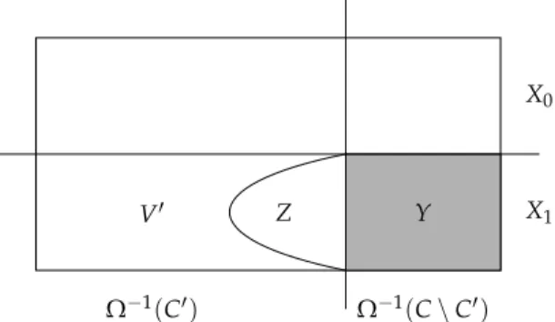
LetY=Ω−1(0)\X1,Z=Attr0(Y)and letabe anattractor strategy for Player 0 which guarantees thatY(or a terminal winning position y ∈ T0) can be reached from every z ∈ Z\Y. Moreover, let V′ = V\(X1∪Z).
The restricted gameG′ = G|V′ has less priorities thanG (since at least all positions with priority 0 have been removed). Thus, by induction hypothesis, the Forgetful Determinacy Theorem holds for G′: V′ =W0′∪W1′and there exist positional winning strategies f′for Player 0 onW0′ andg′for Player 1 onW1′ inG′.
We have thatW1′=∅, as the strategy
g+g′:x7→
g(x) x∈X1 g′(x) x∈W1′
is a positional winning strategy for Player 1 onX1∪W1′. Indeed, every play consistent withg+g′either stays inW1′and is consistent withg′ or reachesX1′ and is from this point on consistent withg. ButX1, by definition, already containsallpositions from which Player 1 can win with a positional strategy, soW1′=∅.
Knowing thatW1′=∅, let f∗= f′+a+f, i.e.
f∗(x) =
f′(x) ifx∈W0′ a(x) ifx∈Z\Y
f(x) ifx∈Y
We claim that f∗ is a positional winning strategy for Player 0 from V\X1. Ifπis a play consistent with f∗, thenπstays inV\X1.
2 Parity Games and Fixed-Point Logics
X1
Y
V′ Z
Ω−1(0)
Figure 2.1.Construction of a winning strategy
Case (a):πhitsZonly finitely often. Thenπeventually stays inW0′and is consistent with f′from this point, so Player 0 winsπ.
Case (b): πhitsZinfinitely often. Thenπalso hitsYinfinitely often, which implies that priority 0 is seen infinitely often. Thus, Player 0
winsπ. q.e.d.
The following theorem is a consequence of positional determinacy.
Theorem 2.7. It can be decided in NP∩coNP whether a given position in a parity game is a winning position for Player 0.
Proof. A node vin a parity gameG = (V,V0,V1,E,Ω)is a winning position for Player σif there exists a positional strategy f :Vσ →V which is winning from positionv. It therefore suffices to show that the question whether a given strategy f :Vσ→Vis a winning strategy for Playerσfrom positionvcan be decided in polynomial time. We prove this for Player 0; the argument for Player 1 is analogous.
GivenG and f :V0→V, we obtain a reduced game graphGf = (W,F)by retaining only those moves that are consistent with f, i.e.,
F={(v,w):(v∈W∩Vσ∧w= f(v))∨ (v∈W∩V1−σ∧(v,w)∈E)}.
In this reduced game, only the opponent, Player 1, makes non- trivial moves. We call a cycle in(W,F)odd if the least priority of its
nodes is odd. Clearly, Player 0 winsGfrom positionvvia strategyf if, and only if, inGfno odd cycle and no terminal positionw∈V0is reach- able fromv. Since the reachability problem is solvable in polynomial
time, the claim follows. q.e.d.
2.1.1 Algorithms for parity games
It is an open question whether winning sets and winning strategies for parity games can be computed in polynomial time. The best algorithms known today are polynomial in the size of the game, but exponential with respect to the number of priorities. Such algorithms run in poly- nomial time when the number of priorities in the input parity game is bounded.
One way to intuitively understand an algorithm solving a parity game is to imagine a judge who watches the players playing the game.
At some point, the judge is supposed to say “Player 0 wins”, and indeed, whenever the judge does so, there should be no question that Player 0 wins. Note that we have no condition in case that Player 1 wins. We will first give a formal definition of a certain kind of judge with bounded memory, and later use this notion to construct algorithms for parity games.
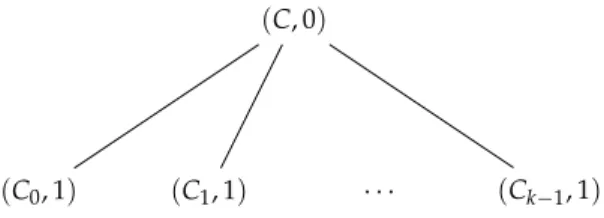
Definition 2.8. A judge M = (M,m0,δ,F) for a parity game G = (V,V0,V1,E,Ω)consists of a set of statesMwith a distinguished initial state m0 ∈ M, a set of final statesF ⊆ M, and a transition function δ : V×M→ M. Note that a judge is thus formally the same as an automaton reading words over the alphabetV. But to be called a judge, two special properties must be fulfilled. Letv0v1. . . be a play ofG andm0m1. . . the corresponding sequence of states ofM, i.e.,m0is the initial state ofMandmi+1=δ(vi,mi). Then the following holds:
(1) ifv0. . . is winning for Player 0, then there is aksuch thatmk∈F, (2) if, for somek,mk∈F, then there existi<j≤ksuch thatvi=vj
and min{Ω(vi+1),Ω(vi+2), . . . ,Ω(vj)}is even.
To illustrate the second condition in the above definition, note that in the playv0v1. . . the sequencevivi+1. . .vjforms a cycle. The judge is
indeed truthful, because both players can use a positional strategy in a parity game, so if a cycle with even priority appears, then Player 0 can be declared as the winner. To capture this intuition formally, we define the following reachability game, which emerges as the product of the original gameGand the judgeM.
Definition 2.9. Let G = (V,V0,V1,E,Ω)be a parity game andM = (M,m0,δ,F) an automaton reading words overV. The reachability gameG × Mis defined as follows:
G × M= (V×M,V0×M,V1×M,E′,V×F),
where((v,m), (v′,m′))∈ E′ iff(v,v′)∈ Eandm′ =δ(v,m), and the last componentV×Fdenotes positions which are immediately winning for Player 0 (the goal of Player 0 is to reach such a position).
Note thatMin the definition above is a deterministic automaton, i.e.,δis a function. Therefore, inGand inG × Mthe players have the same choices, and thus it is possible to translate strategies betweenG andG × M. Formally, for a strategyσinGwe define the strategyσin G × Mas
σ((v0,m0)(v1,m1). . .(vn,mn)) = (σ(v0v1. . .vn),δ(vn,mn)). Conversely, given a strategyσinG × Mwe define the strategyσinG such thatσ(v0v1. . .vn) =vn+1if and only if
σ((v0,m0)(v1,m1). . .(vn,mn)) = (vn+1,mn+1),
wherem0m1. . . is the unique sequence corresponding tov0v1. . ..
Having definedG × M, we are ready to formally prove that the above definition of a judge indeed makes sense for parity games.
Theorem 2.10. Let G be a parity game and Ma judge forG. Then Player 0 winsGfromv0if and only if he winsG × Mfrom(v0,m0). Proof. (⇒) By contradiction, letσbe the winning strategy for Player 0 inG from v0, and assume that there exists a winning strategyρfor
2.1 Parity Games
Player 1 inG × Mfrom(v0,m0). (Note that we just used determinacy of reachability games.) Consider the unique plays
πG =v0v1. . . and πG×M= (v0,m0)(v1,m1). . .
inGandG × M, respectively, which are consistent with bothσandρ (the playπG) and withσandρ(πG×M). Observe that the positions of G appearing in both plays are indeed the same due to the wayσandρ are defined. Since Player 0 winsπG, by Property (1) in the definition of a judge there must be anmk∈ F. But this contradicts the fact that Player 1 winsπG×M.
(⇐) Letσbe a winning strategy for Player 0 inG × M, and letρ be apositionalwinning strategy for Player 1 inG. Again, we consider the unique plays
πG =v0v1. . . πG×M= (v0,m0)(v1,m1). . .
such thatπGis consistent withσandρ, andπG×Mis consistent withσ andρ. SinceπG×Mis won by Player 0, there is anmk∈Fappearing in this play.
By Property (2) in the definition of a judge, there exist two indices i<jsuch thatvi=vjand the minimum priority appearing between vi and vj is even. Let us now consider the following strategyσ′ for Player 0 inG:
σ′(w0w1. . .wn) =
σ(w0w1. . .wn) ifn<j, σ(w0w1. . .wm) otherwise,
wherem=i+ [(n−i) mod(j−i)]. Intuitively, the strategyσ′makes the same choices asσup to the(j−1)st step, and then repeats the choices ofσfrom stepsi,i+1, . . . ,j−1.
We will now show that the unique playπ′inGthat is consistent with bothσ′andρis won by Player 0. Since in the firstjstepsσ′is the same asσ, we have thatπ[n] =vnfor alln≤j. Now observe that π[j+1] =vi+1. Sinceρis positional, ifvjis a position of Player 1, then π[j+1] =vi+1, and ifvjis a position of Player 0, thenπ[j+1] =vi+1
2 Parity Games and Fixed-Point Logics because we definedσ′(v0. . .vj) =σ(v0. . .vi). Inductively repeating this reasoning, we get that the play π repeats the cyclevivi+1. . .vj infinitely often, i.e.
π=v0. . .vi−1(vivi+1. . .vj−1)ω.
Thus, the minimal priority occurring infinitely often inπis the same as min{Ω(vi),Ω(vi+1), . . .Ω(vj−1)}, and thus is even. Therefore Player 0 winsπ, which contradicts the fact thatρwas a winning strategy for
Player 1. q.e.d.
The above theorem allows us, if only a judge is known, to reduce the problem of solving a parity game to the problem of solving a reachability game, which we already tackled with the Gamealgorithm.
But to make use of it, we first need to construct a judge for an input parity game.
The most naïve way to build a judge for afiniteparity gameG is to just remember, for each positionvvisited during the play, what is the minimal priority seen in the play since the last occurrence ofv. If it happens that a positionvis repeated and the minimal priority sincev last occurred is even, then the judge decides that Player 0 won the play.
It is easy to check that an automaton defined in this way indeed is a judge for any finite parity gameG, but such judge can be very big. Since for each of the|V|=n positions we need to store one of
|Ω(V)|=dcolours, the size of the judge is in the order ofO(dn). We will present a judge that is much better for smalld.
Definition 2.11. Aprogress-measuring judgeMP= (MP,m0,δP,FP)for a parity gameG = (V,V0,V1,E,Ω)is constructed as follows. Ifni =
|Ω−1(i)|is the number of positions with priorityi, then
MP={0, 1, . . . ,n0+1} × {0} × {0, 1, . . . ,n2+1} × {0} ×. . . and this product ends in· · · × {0, 1, . . . ,nm+1}if the maximal priority mis even, or in· · · × {0}if it is odd. The initial state ism0= (0, . . . , 0), and the transition functionδ(v,c)withc= (c0, 0,c2, 0, . . . ,cm)is given