2 Parity Games and Fixed-Point Logics

(1)

Logic and Games WS 2018/2019

Prof. Dr. Erich Grädel

Notes and Revisions by Matthias Voit

Mathematische Grundlagen der Informatik RWTH Aachen

(2)

This work is licensed under:

http://creativecommons.org/licenses/by-nc-nd/3.0/de/

Dieses Werk ist lizenziert unter:

http://creativecommons.org/licenses/by-nc-nd/3.0/de/

http://www.logic.rwth-aachen.de

(3)

1 Reachability Games and First-Order Logic

1.1 Model Checking

One of the fundamental algorithmic tasks in logic is model checking.

For a logicLand a domainDof (finite) structures, themodel-checking problemasks, given a structureA∈ Dand a formulaψ∈ L, whether A is a model of ψ. Notice that an instance of the model-checking problem has two inputs: a structure and a formula. We can measure the complexity in terms of both inputs, and this is what is commonly refered to as thecombined complexityof the model-checking problem (forLandD). However, in many cases, one of the two inputs is fixed, and we measure the complexity only in terms of the other. If we fix the structureA, then the model-checking problem forLon this structure amounts to deciding Th_L(A) :={ψ∈ L :A|=ψ}^{, the} L-theoryofA.

The complexity of this problem is called theexpression complexityof the model-checking problem (forL on A). For first-order logic (FO) and for monadic second-order logic (MSO) in particular, such problems have a long tradition in logic and numerous applications in many fields.

Of great importance in many areas of logic, in particular for finite model theory or databases, are model-checking problems for a fixed formulaψ, which amounts to deciding themodel classofψinsideD^, that is Mod_D(ψ):={^A∈ D^:^A|=ψ}. Its complexity is thestructure complexityordata complexityof the model-checking problem (forψon D^).

One of the important themes in this course is a game-based approach to model checking. The general idea is to reduce the problem whetherA|=ψto a strategy problem for amodel checking gameG(A,ψ) played by two players calledVerifier(orPlayer0) andFalsifier(orPlayer1).

(6)

We want to have the following relation between these two problems:

A|=ψ iff Verifier has a winning strategy forG(^A,ψ).

We can then do model checking by constructing, or proving the existence of, winning strategies.

To assess the efficiency of games as a solution for model checking problems, we have to consider the complexity of the resulting model checking games based on the following criteria:

• Are all plays necessarily finite?

• If not, what are the winning conditions for infinite plays?

• Do the players always have perfect information?

• What is the structural complexity of the game graphs?

• How does the size of the graph depend on different parameters of the input structure and the formula?

For first-order logic (FO) and modal logic (ML) we have only finite plays with positional winning conditions, and, as we shall see, the winning regions are computable in linear time with respect to the size of the game graph. Model checking games for fixed-point logics however admit infinite plays, and we use so-calledparity conditionsto determine the winner of such plays. It is still an open question whether winning regions and winning strategies in parity games are computable in polynomial time.

1.2 Model Checking Games for Modal Logic

The first logic that we discuss is propositional modal logic (ML). Let us first briefly review its syntax and semantics:

Definition 1.1. Given a setAof actions and a set{Pi:i∈I}^{of atomic} propositions, the set of formulae of ML is inductively defined:

• All atomic propositionsP_iare formulae of ML.

• Ifψ,φare formulae of ML, then so are¬^ψ,(ψ∧φ)and(ψ∨φ).

• Ifψ∈ML anda∈A, then⟨a⟩ψ∈ML and[a]ψ∈ML.

(7)

1.2 Model Checking Games for Modal Logic Remark1.2. If there is only one action a ∈ A, we write ♢^ψ^and □^ψ instead of⟨a⟩ψand[a]ψ, respectively.

Definition 1.3. Atransition systemorKripke structurewith actions from a setAand atomic properties{Pi:i∈I}is a structure

K= (V,(Ea)_a_∈_A,(Pi)_i_∈_I)

with a universeV of states, binary relationsEa ⊆V×Vdescribing transitions between the states, and unary relationsP_i ⊆Vdescribing the atomic properties of states.

A transition system can be seen as a labelled graph where the nodes are the states of K, the unary relations provide labels of the states, and the binary transition relations can be pictured as sets of labelled edges.

Definition 1.4. Let K = (V,(Ea)_a∈A,(P_i)_i∈I) be a transition system, ψ∈ML a formula andva state ofK^{. The}model relationshipK^,v|=ψ, i.e.,ψholds at statevofK, is inductively defined:

• K,v|=Piif and only ifv∈Pi.

• K^,v|=¬ψif and only ifK^,v̸|=ψ.

• K^,v|=ψ∨φif and only ifK^,v|=ψorK^,v|=φ.

• K^,v|=ψ∧φif and only ifK^,v|=ψandK^,v|=φ.

• K^,v|=⟨a⟩ψif and only if there existswsuch that(v,w)∈Eaand K,w|=ψ.

• K^,v|= [a]ψif and only ifK^,w|=ψholds for allwwith(v,w)∈Ea. For a transition systemKand a formulaψwe define theextension JψK^K:={v:K^,v|=ψ}as the set of states ofK^whereψholds.

For the game-based approach to model-checking, it is convenient to assume that modal formulae are written in negation normal form, i.e.

negation is applied to atomic propositions only. This does not reduce the expressiveness of modal logic since every formula can be efficiently translated into negation normal form by applying De Morgan’s laws and the duality of□^and♢^(i.e. ¬⟨a⟩ψ≡[a]¬ψand¬[a]ψ≡ ⟨a⟩¬^{ψ) to} push negations to the atomic subformulae.

(8)

Syntactically, modal logic is an extension of propositional logic.

However, since ML is evaluated over transition systems, i.e. structures, it is often useful to see it as a fragment of first-order logic.

Theorem 1.5. For each formulaψ∈ML there is a first-order formula ψ^∗(x)(with only two variables), such that for each transition systemK and all its statesvwe have thatK^,v|=ψ⇐⇒ K |=ψ^∗(v).

Proof. The transformation is defined inductively, as follows:

P_i7−→P_ix

¬ψ7−→ ¬ψ^∗(x)

(ψ◦φ)7−→(ψ^∗(x)◦φ^∗(x)), where◦ ∈ {∧,∨,→}

⟨a⟩ψ7−→ ∃y(Eaxy∧ψ^∗(y)) [a]ψ7−→ ∀y(Eaxy→ψ^∗(y))

whereψ^∗(y)is obtained fromψ^∗(x)by interchangingxandyevery-

where in the formula. q.e.d.

We are now ready to describe the model checking games for ML.

Given a transition systemKand a formulaψ∈ML, we define a game G(K^,ψ)whose positions are pairs(φ,v)where φis a subformula of ψand v∈ Vis a node ofK. From any position(φ,v)in this game, Verifier’s goal is to show that K,v |= φ, whereas Falsifier tries to establish thatK^,v̸|=φ.

In the game, Verifier moves at positions of the form(φ∨ϑ,v), with the choice to move either to(φ,v)or to(ϑ,v), and at positions(⟨a⟩^φ,v), where she can move to any position(φ,w)withw∈vEa. Analogously, Falsifier moves from positions(φ∧ϑ,v)to either(φ,v)or(ϑ,v), and from([a]φ,v)to any position(φ,w)withw∈vEa. Finally, at literals, i.e. ifφ=P_iorφ=¬P_i, the position(φ,v)is a terminal position where Verifier has won ifK,v|=φ, and Falsifier has won ifK,v̸|=φ.

The correctness of the construction ofG(K^,ψ)follows readily by induction.

(9)

1.3 Reachability and Safety Games

Proposition 1.6. For any position(φ,v)ofG(K^,ψ)we have that

K^,v|=φ ⇔ Verifier has a winning strategy forG(K^,ψ)from(φ,v). 1.3 Reachability and Safety Games

The model-checking games for propositional modal logic, that we have just discussed, are an instance of reachability games played on graphs or, more precisely, two-player games with perfect information and positional winning conditions, played on agame graph(orarena)

G= (V,V0,V₁,E)

where the setVof positions is partitioned into sets of positionsV0and V1belonging to Player 0 and Player 1, respectively. Player 0 moves from positionsv∈V₀, while Player 1 moves from positionsv∈V₁. All moves are along edges, and so the interaction of the players, starting from an initial positionv0, produces a finite or infiniteplaywhich is a sequence v₀v₁v₂. . . with(v_i,v_i+1)∈Efor alli.

The winning conditions of the players are based on a simple positional principle: Move or lose! This means that Playerσhas won at a positionvin the case that positionvbelongs to his opponent and there are no moves available from that position. Thus the goal of Playerσ is to reach a position inTσ :={v ∈ V1−σ : vE =∅}. We call this a reachability condition.

But note that this winning condition applies to finite plays only.

If the game graph admits infinite plays (for instance cycles) then we must either consider these as draws, or introduce a winning condition for infinite plays. The dual notion of a reachability condition is asafety conditionwhere Playerσjust has the objective to avoid a given set of

‘bad’ positions, which in this case is the setT_1−σ, and to remain inside the safe regionV\T1−σ.

A(positional) strategyfor Playerσin such a gameG is a (partial) function f :{v∈Vσ:vE̸=∅} →Vsuch that(v,f(v))∈ E. A finite or infinite playv0v1v2. . . isconsistent with f ifvi+1=f(vi)for everyi

(10)

such thatv_i∈Vσ. A strategy f for Playerσis winning fromv₀if every play that starts at initial positionv0and that is consistent with fis won by Playerσ.

We first considerreachability gameswhere both players play with the reachability objective to force the play to a position inTσ. We define winning regions

Wσ:={v∈V: Playerσhas a winning strategy from positionv}^. IfW0∪W1 =V, i.e. for eachv∈Vone of the players has a winning strategy, the gameGis calleddetermined. A play which is not won by any of the players is considered a draw.

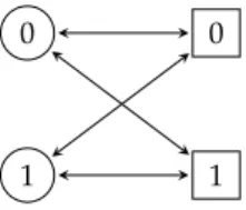
Example1.7. No player can win from one of the middle two nodes:

□ □

The winning regions of a reachability gameG= (V,V0,V1,E)can be constructed inductively as follows:

W_σ⁰=Tσand

W_σⁱ⁺¹=W_σⁱ∪ {v∈Vσ:vE∩W_σⁱ ̸=∅} ∪ {v∈V1−σ:vE⊆W_σⁱ}. ClearlyW_σⁱ is the region of those positions from which Playerσhas a strategy to win in at mostimoves, and for finite game graphs, with

|V|=n, we have thatWσ=W_σⁿ.

Next we consider the case of areachability-safety game, where Player 0, as above, plays with the reachability objective to force the play to a terminal position inT₀, whereas player 1 plays with the safety objective of avoidingT0, i.e. to keep the play inside the safe regionS1:=V\T0. Notice that there are no draws in such a game.

The winning regionW₀of Player 0 can be defined as in the case above, but the winning regionW1of Player 1 is now the maximal set W ⊆ S1 such that from allw ∈WPlayer 1 has a strategy to remain

(11)

1.3 Reachability and Safety Games insideW, which can be defined as the limit of the descending chain W₁⁰⊇W₁¹⊇W₁²⊇^{. . . with}

W₁⁰=S₁and

W₁ⁱ⁺¹=W₁ⁱ∩ {v∈V:(v∈V0andvE⊆W₁ⁱ)or (v∈V₁andvE∩W₁ⁱ̸=∅)}^.

Again on finite game graphs, with|V|=n, we have thatW₁=W_σⁿ. This leads us to two fundamental concepts for the analysis of games on graphs:attractorsandtraps. LetG= (V,V0,V₁,E)be a game graph andX⊆V.

Definition 1.8. Theattractor of X for Playerσ, in short Attr_σ(X)is the set of those positions from which Playerσhas a strategy to reachX(or to win because the opponent cannot move anymore). We can inductively define Attr_σ(X):=^S_n∈NXⁿ, where

X⁰=Xand

Xⁱ⁺¹=Xⁱ∪ {v∈Vσ:vE∩Xⁱ̸=∅} ∪ {v∈V_1−σ:vE⊆Xⁱ}^. For instance, the winning regionWσin a reachability game is the attractor of the winning positions:Wσ=Attr_σ(Tσ).

A setY⊆V\T1−σ=:Sσis called atrapfor Player 1−σif Player σhas a strategy to guarantee that from eachv∈Ythe play will remain insideY. Note that the complement of an attractor Attrσ(X)is a trap for player σ. The maximal trapY of Player 1−σcan be defined as Y=^T_n_∈_NYⁿ, where

Y⁰=Sσand

Yⁱ⁺¹=Yⁱ∩ {v:(v∈VσandvE∩Yⁱ̸=∅)or (v∈V1−σandvE⊆Yⁱ)}^.

The winning region of a Playerσwith the safety objective forSσis the maximal trap for player 1−^σ.

We consider several algorithmic problems for a given reachability

(12)

gameG: The computation of winning regionsW₀andW₁, the computation of winning strategies, and the associated decision problem

Game:={(G^,v): Player 0 has a winning strategy forG^fromv}^. Theorem 1.9. Gameis P-complete and decidable in time O(|V|+|E|).

Note that this remains true forstrictly alternating games.

The inductive definition of an attractor shows that winning regions for both players can be computed efficiently. Hence we can also solve Gamein polynomial time. To solve Gamein linear time, we use the slightly more involved Algorithm 1.1. Procedure Propagate will be called once for every edge in the game graph, so the running time of this algorithm is linear with respect to the number of edges inG^.

Furthermore, we can show that the decision problem Game is equivalent to the satisfiability problem for propositional Horn formulae.

We recall that propositional Horn formulae are finite conjunctions Vi∈ICiof clausesCiof the form

X1∧^{. . .}∧Xn → X or X1∧^{. . .}∧Xn

| {z }

body(Ci)

→ ⁰

head(C|{z}i)

.

A clause of the formXor 1→Xhas an empty body.

We will show that Sat-Hornand Gameare mutually reducible via logspace and linear-time reductions.

(1) Game≤log-linSat-Horn

For a gameG = (V,V₀,V₁,E), we construct a Horn formulaψ_G with clauses

v→u for allu∈V0and(u,v)∈E, and v1∧^{. . .}∧vm→u for allu∈V1anduE={v1, . . . ,vm}^. The minimal model of ψ_G is precisely the winning region of Player 0, so

(G,v)∈Game ⇐⇒ ψ_G∧(v→0)is unsatisfiable.

(13)

1.3 Reachability and Safety Games

Algorithm 1.1.A linear time algorithm for Game Input: A gameG= (V,V0,V1,E)

output: Winning regionsW0andW1

for allv∈Vdo (∗1: Initialisation∗) win[v]:=⊥

P[v]:={u:(u,v)∈E} n[v]:=|vE|

end do

for allv∈V0 (∗2: Calculate win∗) ifn[v] =0thenPropagate(v, 1)

for allv∈V1

ifn[v] =0thenPropagate(v, 0) returnwin

procedurePropagate(v,σ) ifwin[v]̸=⊥then return

win[v]:=σ (∗^{3: Mark}vas winning for playerσ∗) for allu∈P[v]do (∗4: Propagate change to predecessors∗)

n[u]:=n[u]−1

ifu∈Vσorn[u] =0thenPropagate(u,σ) end do

end

(14)

(2) Sat-Horn≤log-linGame

For a Horn formulaψ(X₁, . . . ,Xn) = ^V_i∈IC_i, we define a game Gψ= (V,V0,V1,E)as follows:

V={0} ∪ {X1, . . . ,Xn}

| {z }

V0

∪ {Ci:i∈I}

| {z }

V1

and

E={X→C_i:X=head(C_i)} ∪ {C_i→X_j:X_j∈^body(C_i)}^, i.e., Player 0 moves from a variable to some clause containing the variable as its head, and Player 1 moves from a clause to some variable in its body. Player 0 wins a play if, and only if, the play reaches a clauseCwith body(C) =∅. Furthermore, Player 0 has a winning strategy from positionXif, and only if,ψ|=X, so we have

Player 0 wins from position 0 ⇐⇒ ψis unsatisfiable.

These reductions show that Sat-Hornis also P-complete and, in particular, also decidable in linear time.

1.4 Games as an Algorithmic Construct: Alternating Algorithms Alternating algorithms are algorithms whose set of configurations is divided intoaccepting,rejecting,existentialanduniversalconfigurations.

The acceptance condition of an alternating algorithmAis defined by a game played by two players∃^and∀on the computation graphG(A,x) (or equivalently, the computation treeT(A,x)) ofAon inputx. The positions in this game are the configurations ofA, and we allow moves C→C^′from a configurationCto any of its successor configurations C^′. Player∃moves at existential configurations and wins at accepting configurations, while Player∀moves at universal configurations and wins at rejecting configurations. By definition,Aaccepts some inputx if and only if Player∃has a winning strategy for the game played on TA,x.

We will introduce the concept of alternating algorithms formally, using the model of a Turing machine, and we prove certain relation-

(15)

1.4 Games as an Algorithmic Construct: Alternating Algorithms ships between the resulting alternating complexity classes and usual deterministic complexity classes.

1.4.1 Turing Machines

The notion of an alternating Turing machine extends the usual model of a (deterministic) Turing machine which we introduce first. We consider Turing machines with a separate input tape and multiple linear work tapes which are divided into basic units, called cells or fields. Informally, the Turing machine has a reading head on the input tape and a combined reading and writing head on each of its work tapes.

Each of the heads is at one particular cell of the corresponding tape during each point of a computation. Moreover, the Turing machine is in a certain state. Depending on this state and the symbols the machine is currently reading on the input and work tapes, it manipulates the current fields of the work tapes, moves its heads and changes to a new state.

Formally, a(deterministic) Turing machine with separate input tape and k linear work tapesis given by a tuple M= (Q,Γ,Σ,q₀,Facc,F_rej,δ), where Q is a finite set of states, Σis the work alphabet containing a designated symbol (blank), Γ is the input alphabet, q0 ∈ Q is the initial state, F := Facc∪Frej ⊆ Q is the set of final states(with Facc

the accepting states, Frej the rejecting states and Facc∩Frej = ∅), and δ:(Q\F)×Γ×Σ^k→Q× {−^{1, 0, 1}} ×Σ^k× {−^{1, 0, 1}}^k^{is the}transition function.

AconfigurationofMis a complete description of all relevant facts about the machine at some point during a computation, so it is a tuple C= (q,w₁, . . . ,w_k,x,p0,p₁, . . . ,p_k) ∈Q×(Σ^∗)^k×Γ^∗×^N^k+1^whereq is the current state,wiis the contents of work tape numberi,xis the contents of the input tape,p₀is the position on the input tape andp_iis the position on work tape numberi. The contents of each of the tapes is represented as a finite word over the corresponding alphabet[, i.e., a finite sequence of symbols from the alphabet]. The contents of each of the fields with numbersj>|w_i|on work tape numberiis the blank symbol (we think of the tape as being infinite). A configuration wherex

(16)

is omitted is called apartial configuration. The configurationCis called finalifq∈F. It is calledacceptingifq∈Faccandrejectingifq∈Frej.

The successor configuration of C is determined by the current state and the k+1 symbols on the current cells of the tapes, using the transition function: Ifδ(q,xp0,(w1)_p₁, . . . ,(w_k)_p_k) = (q^′,m0,a1, . . . ,ak,m1, . . . ,mk,b), then the successor configuration ofC is ∆(C) = (q^′,w^′,p^′,x), where for any i, w^′_i is obtained fromw_i by replacing symbol number pibyaiandp^′_i=pi+mi. We writeC⊢MC^′ if, and only if,C^′=∆(C).

Theinitial configuration C0(x) =C0(M,x)ofMon inputx∈Γ^∗is given by the initial stateq0, the blank-padded memory, i.e.,wi=εand p_i=0 for anyi≥^1,p₀=0, and the contentsxon the input tape.

AcomputationofMon inputxis a sequenceC0,C1, . . . of configurations of M, such that C₀ = C₀(x) and C_i ⊢M C_i+1 for all i ≥ ^0.

The computation is calledcompleteif it is infinite or ends in some final configuration. A complete finite computation is calledacceptingif the last configuration is accepting, and the computation is calledrejecting if the last configuration is rejecting. M acceptsinputxif the (unique) complete computation ofMonxis finite and accepting. M rejectsinput xif the (unique) complete computation ofMonxis finite and rejecting.

The machineM decidesa languageL⊆Γ^∗ifMaccepts allx∈Land rejects allx∈Γ^∗\L.

1.4.2 Alternating Turing Machines

Now we shall extend deterministic Turing machines to nondeterministic Turing machines from which the concept of alternating Turing machines is obtained in a very natural way, given our game theoretical framework.

Anondeterministic Turing machineis nondeterministic in the sense that a given configurationCmay have several possible successor configurations instead of at most one. Intuitively, this can be described as the ability toguess. This is formalised by replacing the transition function δ:(Q\F)×Γ×Σ^k→Q× {−^{1, 0, 1}} ×Σ^k× {−^{1, 0, 1}}^kby a transition relation∆⊆((Q\F)×Γ×Σ^k)×(Q× {−^{1, 0, 1}} ×Σ^k× {−^{1, 0, 1}}^k). The notion of successor configurations is defined as in the deterministic

(17)

1.4 Games as an Algorithmic Construct: Alternating Algorithms case, except that the successor configuration of a configurationCmay not be uniquely determined. Computations and all related notions carry over from deterministic machines in the obvious way. However, on a fixed inputx, a nondeterministic machine now has several possible computations, which form a (possibly infinite) finitely branching computation treeTM,x. A nondeterministic Turing machineM accepts an inputxif thereexistsa computation ofMonxwhich is accepting, i.e., if there exists a path from the rootC0(x)ofTM,x to some accepting configuration. The language of MisL(M) ={x∈Γ^∗| Macceptsx}. Notice that for a nondeterministic machine Mto decide a language L⊆Γ^∗ it is not necessary that all computations ofMare finite. (In a sense, we count infinite computations as rejecting.)

From a game-theoretical perspective, the computation of a nondeterministic machine can be viewed as a solitaire game on the computation tree in which the only player (the machine) chooses a path through the tree starting from the initial configuration. The player wins the game (and hence, the machine accepts its input) if the chosen path finally reaches an accepting configuration.

An obvious generalisation of this game is to turn it into a two- player game by assigning the nodes to the two players who are called∃ and∀, following the intuition that Player∃tries to show the existence of agoodpath, whereas Player ∀tries to show that all selected paths arebad. As before, Player∃wins a play of the resulting game if, and only if, the play is finite and ends in an accepting leaf of the game tree.

Hence, we call a computation tree accepting if, and only if, Player∃^has a winning strategy for this game.

It is important to note that the partition of the nodes in the tree should not depend on the inputxbut is supposed to be inherent to the machine. Actually, it is even independent of the contents of the work tapes, and thus, whether a configuration belongs to Player∃^{or to} Player∀merely depends on the current state.

Formally, analternating Turing machineis a nondeterministic Turing machine M= (Q,Γ,Σ,q0,Facc,Frej,∆) whose set of statesQ = Q_∃∪ Q_∀∪Facc∪Frejis partitioned into existential, universal, accepting, and

(18)

rejectingstates. The semantics of these machines is given by means of the game described above.

Now, if we let accepting configurations belong to player ∀and rejecting configurations belong to player ∃, then we have the usual winning condition that a player loses if it is his turn but he cannot move.

We can solve such games by determining the winner at leaf nodes and propagating the winner successively to parent nodes. If at some node, the winner at all of its child nodes is determined, the winner at this node can be determined as well. This method is sometimes referred to as backwards induction and it basically coincides with our method for solving Gameon trees (with possibly infinite plays). This gives the following equivalent semantics of alternating Turing machines:

The subtreeTCof the computation tree ofMon xwith rootCis calledaccepting, if

• Cis accepting

• Cis existential and there is a successor configurationC^′ofCsuch thatTC^′is accepting or

• Cis universal andTC^′ is accepting for all successor configurations C^′ofC.

Maccepts an inputx, ifT_C₀_(x)=TM,xis accepting.

For functionsT,S:N→N, an alternating Turing machineMis calledT-time boundedif, and only if, for any inputx, each computation of Mon x has length less or equalT(|x|). The machine is called S- space boundedif, and only if, for any inputx, during any computation of Mon x, at mostS(|x|) cells of the work tapes are used. Notice that time boundedness implies finiteness of all computations which is not the case for space boundedness. The same definitions apply for deterministic and nondeterministic Turing machines as well since these are just special cases of alternating Turing machines. These notions of resource bounds induce the complexity classes Atime containing precisely those languages L such that there is an alternating T-time bounded Turing machine decidingLand Aspacecontaining precisely those languages Lsuch that there is an alternatingS-space bounded

(19)

1.4 Games as an Algorithmic Construct: Alternating Algorithms Turing machine decidingL. Similarly, these classes can be defined for nondeterministic and deterministic Turing machines.

We are especially interested in the following alternating complexity classes:

• ALogspace=^S_d∈NAspace(d·^logn),

• APtime=^S_d∈NAtime(n^d),

• APspace=^S_d_∈_NAspace(n^d).

Observe that Game∈Alogspace. An alternating algorithm which decides Gamewith logarithmic space just plays the game. The algorithm only has to store thecurrentposition in memory, and this can be done with logarithmic space. We shall now consider a slightly more involved example.

Example1.10. QBF ∈^Atime(O(n)). W.l.o.g we assume that negation appears only at literals. We describe an alternating procedureEval(φ,I) which computes, given a quantified Boolean formulaψand a valuation I^{: free}(ψ)→ {^{0, 1}}of the free variables ofψ, the valueJψK^I.

Algorithm 1.2.Alternating algorithm deciding QBF.

Input:(ψ,I) ^whereψ∈^{QAL and}I^{: free}(ψ)→ {^{0, 1}} ifψ=Y then

ifI(Y) =1thenaccept elsereject

ifψ=φ1∨φ2 then„∃^{“ guesses}i∈ {^{1, 2}}^,Eval(φ_i,I) ifψ=φ₁∧φ₂ then„∀^{“ chooses}i∈ {^{1, 2}}^,Eval(φ_i,I) ifψ=∃Xφ then„∃“ guessesj∈ {0, 1},Eval(φ,I[X=j]) ifψ=∀Xφ then„∀^{“ chooses}j∈ {^{0, 1}}^,Eval(φ,I[X=j])

1.4.3 Alternating versus Deterministic Complexity Classes

The main results we want to establish in this section concern the relationship between alternating complexity classes and deterministic complexity classes. We will see that alternating time corresponds to

(20)

deterministic space, while by translating deterministic time into alternating space, we can reduce the complexity by one exponential. Here, we consider the special case of alternating polynomial time and polynomial space. We should mention, however, that these results can be generalised to arbitrary large complexity bounds which are well behaved in a certain sense.

Lemma 1.11. NPspace⊆^APtime.

Proof. Let L ∈ ^NPspace ^{and let} M be a nondeterministic n^l-space bounded Turing machine which recognises L for somel ∈ N. The machineMaccepts some inputxif, and only if, some accepting configuration is reachable from the initial configurationC0(x)in the configuration tree ofMonxin at mostk:=2^cn^l steps for somec∈^{N. This is} due to the fact that there are mostkdifferent configurations ofMon inputxwhich use at mostn^l cells of the memory which can be seen using a simple combinatorial argument. So if there is some accepting configuration reachable from the initial configurationC0(x), then there is some accepting configuration reachable fromC0(x)in at mostksteps.

This is equivalent to the existence of some intermediate configuration C^′ that is reachable fromC0(x) in at most^k/2steps and from which some accepting configuration is reachable in at most^k/2steps.

So the alternating algorithm decidingLproceeds as follows. The existential player guesses such a configuration C^′ and the universal player chooses whether to check thatC^′is reachable fromC0(x)in at most^k/2steps or whether to check that some accepting configuration is reachable fromC^′in at most^k/2steps. Then the algorithm (or equivalently, the game) proceeds with the subproblem chosen by the universal player, and continues in this binary search like fashion. Obviously, the number of steps which have to be performed by this procedure to decide whether xis accepted byMis logarithmic ink. Sincekis exponential inn^l, the time bound of Misdn^l for somed∈^{N, so} M

decidesLin polynomial time. q.e.d.

Lemma 1.12. APtime⊆Pspace.

(21)

1.4 Games as an Algorithmic Construct: Alternating Algorithms Proof. Let L ∈^APtime^{and let} Abe an alternating n^l-time bounded Turing machine that decidesL for somel ∈ N. Then there is some r∈^Nsuch that any configuration ofAon any inputxhas at mostr successor configurations and w.l.o.g. we can assume that any non-final configuration has preciselyrsuccessor configurations. We can think of the successor configurations of some non-final configurationCas being enumerated asC₁, . . . ,Cr. Clearly, for givenCandiwe can computeC_i. The idea for a deterministic Turing machineMto check whether some inputxis inLis to perform a depth-first search on the computation tree TA,x of A on x. The crucial point is that we cannot construct and keep the whole configuration treeTA,xin memory since its size is exponential in|x|which exceeds our desired space bound. However, since the length of each computation is polynomially bounded, it is possible to keep a single computation path in memory and to construct the successor configurations of the configuration under consideration on the fly.

Roughly, the procedureMcan be described as follows. We start with the initial configurationC₀(x). Given any configurationCunder consideration, we propagate 0 to the predecessor configuration ifCis rejecting and we propagate 1 to the predecessor configuration ifCis accepting. If Cis neither accepting nor rejecting, then we construct, fori=1, . . . ,rthe successor configurationC_iofCand proceed with checkingCi. IfCis existential, then as soon as we receive 1 for somei, we propagate 1 to the predecessor. If we encounter 0 for alli, then we propagate 0. Analogously, ifCis universal, then as soon as we receive a 0 for somei, we propagate 0. If we receive only 1 for alli, then we propagate 1. Thenxis inLif, and only if, we finally receive 1 atC0(x). Now, at any point during such a computation we have to store at most one complete computation ofAonx. SinceAisn^l-time bounded, each such computation has length at mostn^land each configuration has size at mostc·n^lfor somec∈N. SoMneeds at mostc·n^2lmemory cells

which is polynomial inn. q.e.d.

So we obtain the following result.

Theorem 1.13. (Parallel time complexity = sequential space complexity)

(22)

(1) APtime=Pspace.

(2) AExptime=Expspace.

Proposition (2) of this theorem is proved exactly the same way as we have done it for proposition (1). Now we prove that by translating sequentialtimeinto alternatingspace, we can reduce the complexity by one exponential.

Lemma 1.14. Exptime⊆^APspace

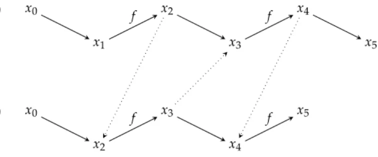
Proof. LetL∈Exptime. Using a standard argument from complexity theory, there is a deterministic Turing machine M= (Q,Σ,q0,δ)with time boundm:=2^c·n^kfor somec,k∈^Nwith only a single tape (serving as both input and work tape) which decides L. (The time bound of the machine with only a single tape is quadratic in that of the original machine withkwork tapes and a separate input tape, which, however, does not matter in the case of an exponential time bound.) Now if Γ=Σ⊎(Q×Σ)⊎ {^#}, then we can describe each configurationCof Mby a word

C=#w₀. . .w_i₋₁(qw_i)w_i+1. . .wt#∈Γ^∗.

SinceMhas time boundmand only one single tape, it has space bound m. So, w.l.o.g., we can assume that|C|=m+2 for all configurations Cof M on inputs of lengthn. (We just use a representation of the tape which has a priori the maximum length that will occur during a computation on an input of lengthn.) Now the crucial point in the argumentation is the following. If C ⊢ C^′ and 1 ≤ i ≤ m, symbol numberiof the wordC^′only depends on the symbols numberi−^1, iandi+1 ofC. This allows us to decide whetherx∈L(M)with the following alternating procedure which uses only polynomial space.

Player∃guesses some numbers≤mof steps of which he claims that it is precisely the length of the computation of Mon input x.

Furthermore, ∃ guesses some state q ∈ Facc, a Symbol a ∈ Σ and a number i ∈ {^{0, . . . ,}s}, and he claims that the i-th symbol of the configurationCofMafter the computation onxis(qa). (So players start inspecting the computation ofMonxfrom the final configuration.)

(23)

1.4 Games as an Algorithmic Construct: Alternating Algorithms IfMaccepts inputx, then obviously player∃has a possibility to choose all these objects such that his claims can be validated. Player∀^{wants to} disprove the claims of∃. Now, player∃guesses symbolsa₋1,a0,a1∈Γ of which he claims that these are the symbols numberi−^1,iandi+1 of the predecessor configuration of the final configuration C. Now,

∀can choose any of these symbols and demand that∃validates his claim for this particular symbol. This symbol is now the symbol under consideration, while iis updated according to the movement of the (unique) head of M. Now, these actions of the players take place for each of the scomputation steps of M on x. After ssuch steps, we check whether the current symbol and the current position are consistent with the initial configurationC₀(x). The only information that has to be stored in the memory is the positionion the tape, the numberswhich∃has initially guessed and the current number of steps.

Therefore, the algorithm uses space at most O(log(m)) =O(n^k)which is polynomial inn. Moreover, ifMaccepts inputxthen obviously player

∃has a winning strategy for the computation game. If, conversely,M rejects inputx, then the combination of all claims of player∃^{cannot be} consistent and player∀has a strategy to spoil any (cheating) strategy of player ∃by choosing the appropriate symbol at the appropriate

computation step. q.e.d.

Finally, we make the simple observation that it is not possible to gain more than one exponential when translating from sequential time to alternating space. (Notice that Exptimeis a proper subclass of 2Exptime.)

Lemma 1.15. APspace⊆^Exptime

Proof. LetL∈APspace, and letAbe an alternatingn^k-space bounded Turing machine which decidesL for somek ∈ N. Moreover, for an input xof A, let Conf(A,x) be the set of all configurations ofAon input x. Due to the polynomial space bound of A, this set is finite and its size is at most exponential in |x|. So we can construct the graph G = (Conf(A,x),⊢) in time exponential in |x|. Moreover, a configuration C is reachable from C0(x) in TA,x if and only if C is

(24)

reachable fromC₀(x)inG. So to check whetherAaccepts inputxwe simply decide whether player∃has a winning strategy for the game played onGfromC0(x). This can be done in time linear in the size of G, so altogether we can decide whetherx∈L(A)in time exponential

in|x|^. ^q.e.d.

Theorem 1.16. (Translating sequential time into alternating space) (1) ALogspace=P.

(2) APspace=Exptime.

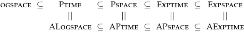
Proposition (1) of this theorem is proved using exactly the same arguments as we have used for proving proposition (2). An overview over the relationship between deterministic and alternating complexity classes is given in Figure 1.1.

Logspace ⊆ ^Ptime ⊆ ^Pspace ⊆ ^Exptime ⊆ ^Expspace

|| || || ||

ALogspace ⊆ ÂPtime ⊆ ÂPspace ⊆ ÂExptime

Figure 1.1.Relation between deterministic and alternating complexity classes

1.5 Model Checking Games for First-Order Logic

Let us first recall the syntax of FO formulae on relational structures.

We have thatR_i(x¯),¬R_i(x¯),x=yandx̸=yare well-formed valid FO formulae, and inductively for FO formulaeφandψ, we have thatφ∨^ψ, φ∧^ψ,∃xφand∀xφare well-formed FO formulae. This way, we allow only formulae innegation normal formwhere negations occur only at atomic subformulae and all junctions except∨^and∧are eliminated.

These constraints do not limit the expressiveness of the logic, but the resulting games are easier to handle.

For a structureA= (A,R₁, . . . ,Rm)withR_i ⊆A^rⁱ, we define the evaluation gameG(A,ψ)as follows:

We have positionsφ(a¯)for every subformulaφ(x¯)ofψand every a¯∈A^k.

(25)

1.5 Model Checking Games for First-Order Logic At a positionφ∨ϑ, Verifier can choose to move either toφor to ϑ, while at positions∃xφ(x, ¯b), he can choose an instantiationa∈Aof xand move toφ(a, ¯b). Analogously, Falsifier can move from positions φ∧ϑ to either φorϑand from positions ∀xφ(x, ¯b)to φ(a, ¯b)for an a∈A.

The winning condition is evaluated at positions with atomic or negated atomic formulaeφ, and we define that Verifier wins atφ(a¯)if, and only if,A|=φ(a¯), and Falsifier wins if, and only if,A̸|=φ(a¯).

In order to determine the complexity of FO model checking, we have to consider the process of determining whetherA|=ψ. To decide this question, we have to construct the gameG(A,ψ)and check whether Verifier has a winning strategy from positionψ. The size of the game graph is bound by |G(A,ψ)| ≤ |ψ| · |A|^width(ψ), where width(ψ) is the maximal number of free variables in the subformulae of ψ. So the game graph can be exponential, and therefore we can get only exponential time complexity for Game. In particular, we have the following complexities for the general case:

• alternating time:O(|ψ|+qd(ψ)log|A|) where qd(ψ)is the quantifier-depth ofψ,

• alternating space:O(width(ψ)·^log|A|+log|ψ|),

• deterministic time:O(|ψ| · |A|^width(ψ))and

• deterministic space:O(|ψ|+qd(ψ)log|A|).

Efficient implementations of model checking algorithms will construct the game graph on the fly while solving the game.

We obtain that the structural complexity of FO model checking is ALogtime, and both the expression complexity and the combined complexity are PSpace.

Fragments ofFOwith Efficient Model Checking

We have seen that the size of the model checking games for first- order fomulae is exponential with respect to the width of the formulae, so we do not obtain polynomial-time model-checking algorithms in the general case. We now consider appropriate restrictions of FO, that lead to fragments with small model-checking games and thus to efficient game-based model-checking algorithms.

(26)

Thek-variable fragment ofFO is FO^k:={ψ∈^{FO : width}(ψ)≤k}^.

Clearly |G(^A,ψ)| ≤ |ψ| · |A|^k for any finite structureAand any ψ∈^FO^k^.

Theorem 1.17. ModCheck(FO^k)is solvable in timeO(|ψ| · |A|^k) and P-complete, for everyk≥^2.

As shown in Theorem 1.5, modal logic can be embedded (efficiently) into FO². Hence, also ML model checking has polynomial time complexity.

It is a general observation that modal logics have many convenient model-theoretic and algorithmic properties. Besides efficient model- checking the following facts are important in many applications of modal logic.

• The satisfiability problem for ML is decidable (in PSpace),

• ML has the finite model property: each satisfiable formula has a finite model,

• ML has the tree model property: each satisfiable formula has a tree-shaped model,

• algorihmic problems for ML can be solved by automata-based methods.

The embedding of ML into FO²has sometimes been proposed as an explanation for the good properties of modal logic, since FO²is a first- order fragment that shares some of these properties. However, more recently, it has been seen that this explanation has its limitations and is not really convincing. In particular, there are many extensions of ML to temporal and dynamic logics such as LTL, CTL, CTL^∗, PDL and the µ-calculus L_µthat are of great importance for applications in computer science, and that preserve many of the good algorithmic properties of ML. Especially the associated satisfiability problems remain decidable.

However this is not at all true for the corresponding extension of FO². A better and more recent explanation for the good properties of modal logic is that modal operators correspond to a restricted form of

(27)

1.5 Model Checking Games for First-Order Logic quantification, namelyguarded quantification. Indeed, in the embedding of ML into FO², all quantifiers areguardedby atomic formulae. This can be vastly generalised beyond two-variable logic and involving formulae of arbitrary relational vocabularies, leading to theguarded fragmentof FO.

Definition 1.18. The guarded fragment of first-order logic GF is the fragment of first-order logic which allows only guarded quantification

∃y^¯(α(x, ¯¯ y)∧φ(x, ¯¯ y))and∀y^¯(α(x, ¯¯ y)→φ(x, ¯¯ y)),

where theguardsαare atomic formulae containing all free variables ofφ.

GF is a generalisation of modal logics: ML⊆^GF⊆FO. Indeed, the modal operators♢^and□can be expressed as

⟨a⟩φ≡ ∃y(Eaxy∧φ(y))and[a]φ≡ ∀y(Eaxy→φ(y)).

It has turned out that the guarded fragment preserves (and ex- plains to some extent) essentially all of the good model-theoretic and algorithmic properties of modal logics, in a far more expressive setting.

In terms of model-checking games, we can observe that guarded logics have small model checking games of size ∥G(A,ψ)∥ = O(|ψ| · ∥^A∥), and so there exist efficient game-based model-checking algorithms for them.

(28)

(29)

2 Parity Games and Fixed-Point Logics

In the first chapter we have discussed model checking games for first- order logic and modal logic. These games admit only finite plays and their winning conditions are specified just by sets of positions, that the players want to reach. Winning regions in these games can be computed in linear time with respect to the size of the game graph.

However, in many computer science applications, more expressive logics are needed, such as temporal logics, dynamic logics, fixed-point logics and others. Model checking games for these logics admit infinite plays and their winning conditions must be specified in a more elaborate way. As a consequence, we have to consider the theory of infinite games.

For fixed-point logics, such as LFP or the modalµ-calculus, the appropriate evaluation games are parity games. These are games of possibly infinite duration with a function that assigns to each position a natural number, called itspriority. The winner of an infinite play is determined according to whether the least priority seen infinitely often during the play is even or odd.

2.1 Parity Games

Definition 2.1. Aparity gameis given by a labelled game graphG = (V,V0,V₁,E,Ω)as in Sect. 1.3 with a functionΩ:V→^Nthat assigns a priorityto each position. The setVof positions may be finite or infinite, but|Ω(V)|, the number of different priorities which is called theindex ofG, must be finite. As before, a finite play is lost by the player who gets stuck, i.e. cannot move. For infinite playsv0v1v2. . ., we have the parity winning condition: If the least number appearing infinitely often in the sequenceΩ(v0)Ω(v1). . . of priorities is even, then Player 0 wins the play, otherwise Player 1 wins.

(30)

A strategy (for Playerσ) is a function f : V^∗Vσ → V such that f(v0v₁. . .vn)∈vnE. We say that a playπ=v0v₁. . . isconsistentwith the strategy f of Playerσ if for each vi ∈ Vσ it holds thatvi+1 = f(v₀. . .v_i). The strategy f iswinningfor Playerσfrom (or on) a set W ⊆Vif each play starting inWthat is consistent with f is won by Playerσ.

In general, a strategy may depend on the entire history played so far, and can thus be a very complicated object. However, we are interested in simple strategies that depend only on the current position.

Definition 2.2. A strategy (of Playerσ) is calledpositional(ormemoryless) if it only depends on the current position, but not on the history of the play, which means that f(hv) = f(h^′v)for allh,h^′∈V^∗,v∈V. We can view positional strategies simply as functions f :Vσ→V.

We shall see that positional strategies suffice to solve parity games.

Before we formulate and prove this Forgetful Determinacy Theorem, we recall that positional strategies are of course sufficient whenever, as in the previous chapter, the players have purely positional objectives such as reachability or safety. Specifically, for every gameG= (V,V0,V1,E) and everyX⊆Vwe have defined the attractor

Attr_σ(X) ={v∈V: Playerσhas a strategy fromvto reach some positionx∈X∪Tσ}

and such anattractor strategycan, without loss of generality, assumed to be positional. Similarly, ifY⊆Vis atrapfor Playerσ, then Player (1−σ)has a positionaltrap strategyto keep the play insideY.

Further we note that positional winning strategies on parts of the game graph may be combined to positional winning strategies on larger regions. Indeed, let f and f^′be positional strategies for Playerσthat are winning exactly on the setsW,W^′, respectively. Let(f+f^′)be the positional strategy defined by

(f+f^′)(x):=





f(x) ifx∈W f^′(x) otherwise.

(31)

2.1 Parity Games Then(f+f^′)is a winning strategy onW∪W^′.

We can now turn to the proof of the Forgetful Determinacy Theo- rem.

Theorem 2.3(Forgetful Determinacy). In any parity game, the set of positions can be partitioned into two setsW0andW1such that Player 0 has a positional strategy that is winning on W₀ and Player 1 has a positional strategy that is winning onW1.

Proof. Let G = (V,V0,V1,E,Ω) be a parity game with |Ω(V)| = m.

Without loss of generality we can assume thatΩ(V) ={^{0, . . . ,}m−¹} or Ω(V) = {^{1, . . . ,}m}. We prove the statement by induction over

|Ω(V)|^.

In the case that |Ω(V)| = 1, i.e., Ω(V) = {⁰} ^or Ω(V) = {¹}^, either Player 0 or Player 1 wins every infinite play. Her opponent can only win by reaching a terminal position that does not belong to him.

So we have, forΩ(V) ={σ}^, W_1−σ=Attr_1−σ(T_1−σ)and W_σ =V\W_1−σ.

ComputingW_1−σas the attractor ofT_1−σis a simple reachability problem, and thus it can be solved with a positional strategy. ForWσthere is a positional strategy that avoids leaving this (1−σ)-trap.

Let now |Ω(v)| = m > 1. We explicitly consider the case that 0 ∈ Ω(V), i.e., Ω(V) = {^{0, . . . ,}m−¹}. Otherwise, if the minimal priority is 1, we can use the same argumentation with switched roles of the players. We define

X₁:={v∈V: Player 1 has a positional winning strategy fromv}^, and letgbe a positional winning strategy for Player 1 onX₁.

Our goal is to provide a positional winning strategy f^∗for Player 0 onX₀:=V\X₁, so in particular we haveW₁=X₁andW₀=V\X₁.

First of all, observe thatX0is a trap for Player 1. Indeed, if Player 1 could reach X1 from somev ∈ X0, then Player 1 could win with a

(32)

positional strategy fromv, sovwould also be inX₁. Thus, there exists a positionaltrap strategy tfor Player 0 onX0that guarantees that a play remains insideX0.

LetY=Ω⁻¹(0)∩X0andZ=Attr₀(Y). Player 0 has a positional attractor strategyato ensure, from every positionz∈Z\Y, thatY(or a terminal winning position inT0) is reached in finitely many steps.

Let nowV^′ =V\(X1∪Z). The restricted gameG^′ = G|V^′ has strictly fewer priorities thanG(since at least all positions with priority 0 have been removed). Thus, by induction hypothesis, the Forgetful Determinacy Theorem holds forG^′. This means thatV^′=W₀^′∪W₁^′ and there exist positional winning strategies f^′for Player 0 onW₀^′ andg^′ for Player 1 onW₁^′inG^′^.

However, it follows thatW₁^′=∅, since the strategy

(g+g^′):x7→





g(x) x∈X₁ g^′(x) x∈W₁^′

is a positional winning strategy for Player 1 onX₁∪W₁^′. Indeed, every play consistent with(g+g^′)either stays inW₁^′and is consistent with g^′or reachesX1and is from this point on consistent withg. ButX1, by definition, already containsallpositions from which Player 1 can win with a positional strategy, soW₁^′ =∅.

X1

Y

V^′ Z

Ω⁻¹(0)

Figure 2.1.Construction of a winning strategy

Knowing thatW₁^′=∅, let f^∗= f^′+a+t, i.e.

(33)

2.1 Parity Games

f^∗(x) =









f^′(x) ifx∈W₀^′ a(x) ifx∈Z\Y t(x) ifx∈Y

We claim thatf^∗is a positional winning strategy for Player 0 fromX₀. Note that ifπis a play that is consistent with f^∗, thenπremains inside X0. We distinguish two cases.

Case (a):πhitsZonly finitely often. Thenπeventually stays inW₀^′and is consistent with f^′from this point onwards. Hence Player 0 winsπ.

Case (b): πhitsZinfinitely often. Thenπalso hitsYinfinitely often, which implies that priority 0 is seen infinitely often. Thus, Player 0

winsπ. q.e.d.

The following theorem is a consequence of positional determinacy.

Theorem 2.4. It can be decided in NP∩coNP whether a given position in a parity game is a winning position for Player 0.

Proof. A node vin a parity game G = (V,V0,V1,E,Ω) is a winning position for Playerσif there exists a positional strategy f :Vσ →V which is winning from positionv. It therefore suffices to show that the question whether a given strategy f:Vσ→Vis a winning strategy for Playerσfrom positionvcan be decided in polynomial time. We prove this for Player 0; the argument for Player 1 is analogous.

GivenG ^and f :V₀ →V, we obtain a reduced game graphGf = (W,F)by retaining only those moves that are consistent with f, i.e.,

F={(v,w):(v∈W∩Vσ∧w= f(v))∨ (v∈W∩V_1−σ∧(v,w)∈E)}^.

In this reduced game, only the opponent, Player 1, makes non- trivial moves. We call a cycle in(W,F)odd if the least priority of its nodes is odd. Clearly, Player 0 winsGfrom positionvvia strategyf if, and only if, inGfno odd cycle and no terminal positionw∈V₀is reachable fromv. Since the reachability problem is solvable in polynomial

time, the claim follows. q.e.d.

(34)

2.2 Algorithms for parity games

It is an open question whether winning sets and winning strategies for parity games can be computed in polynomial time. The best algorithms known today are polynomial in the size of the game, but exponential with respect to the number of priorities. On an class of parity games with bounded index, such algorithms run in polynomial time.

One way to intuitively understand an algorithm solving a parity game is to imagine a referee who watches the players playing the game.

At some point, the referee is supposed to say “Player 0 wins”, and indeed, whenever the referee does so, there should be no question that Player 0 wins. We shall first give a formal definition of a certain kind of referee with bounded memory, and later use this notion to construct algorithms for parity games.

Definition 2.5. Areferee M = (M,m0,δ,F) for a parity game G = (V,V0,V1,E,Ω)consists of a set of statesMwith a distinguished initial state m0 ∈ M, a set of final states F ⊆ M, and a transition function δ : V×M→ M. Note that a referee is thus formally the same as an automaton reading words over the alphabetV. But to be called a referee, two further conditions must be satisfied, for any playv0v₁. . . of G, and and the corresponding sequencem0m1. . . of states ofM^{, where} m₀is the initial state ofM^andm_i+1=δ(v_i,m_i):

(1) Ifv₀. . . is winning for Player 0, then there is aksuch thatm_k∈F, (2) Ifm_k∈Ffor somek, then there existi<j≤ksuch thatv_i=v_j

and min{Ω(vi+1),Ω(vi+2), . . . ,Ω(vj)}^{is even.}

To illustrate the second condition in the above definition, note that in the playv₀v₁. . . the sequencev_iv_i+1. . .v_jforms a cycle. Assuming that both players use a positional strategy the decision of the referee is correct. Indeed, if a cycle with even priority appears, then this cycle will be repeated forever, Player 0 can be declared as the winner. To capture this intuition formally, we define the following reachability game, which emerges as the product of the original gameG and the refereeM. Definition 2.6. LetG = (V,V0,V1,E,Ω) be a parity game andM= (M,m0,δ,F)an automaton reading words overV. We associate withG

(35)

2.2 Algorithms for parity games

andMa reachability game

G × M= (V×M,V₀×M,V₁×M,E^′,V×F),

where((v,m), (v^′,m^′))∈E^′iff(v,v^′)∈Eandm^′=δ(v,m), andV×F is the set of positions which are immediately winning for Player 0 (the goal of Player 0 is to reach such a position). Plays that do not reach a position inV×Fare won by Player 1.

Note thatMin the definition above is a deterministic automaton, i.e.,δis a function. Therefore, inGand inG × Mthe players have the same choices, and thus it is possible to translate strategies betweenG andG × M. Formally, for a strategy finGwe define the strategy f in G × Mas

f((v0,m0)(v1,m1). . .(vn,mn)) = (f(v0v1. . .vn),δ(vn,mn)). Conversely, given a strategy f inG × Mwe define the strategy f inG such that f(v₀v₁. . .vn) =v_n+1if and only if

f((v₀,m₀)(v₁,m₁). . .(vn,mn)) = (v_n+1,m_n+1),

wherem₀m₁. . . is the unique sequence corresponding tov₀v₁. . ..

WithG × Mwe are ready to prove that the definition of a referee indeed makes sense for parity games.

Theorem 2.7. LetG be a parity game and Ma referee forG. Then Player 0 winsG^fromv₀if, and only if, she winsG × M^from(v₀,m₀). Proof. (⇒^{) Let}fbe a winning strategy for Player 0 inG^fromv0. Assume that Player 0 does not have a winning strategy forG × M^from(v0,m0). By determinacy of reachability games, there exists a winning strategyg for Player 1. Consider the unique playπ_G =v0v1. . . that is consistent with fandgand the unique playπ_G×M= (v0,m0)(v1,m1). . . which is consistent with f andg. Observe that the positions ofG^appearing in both plays are indeed the same due to the way fandgare defined.

Since Player 0 wins π_G, by Property (1) in the definition of a referee

2 Parity Games and Fixed-Point Logics

Logic and Games WS 2018/2019

Contents

1 Reachability Games and First-Order Logic

2 Parity Games and Fixed-Point Logics