Scalable Triangle Counting and LCC with Caching

Research Collection

Bachelor Thesis

Scalable Triangle Counting and LCC with Caching

Author(s):

Strausz, András Publication Date:

2021-03-05 Permanent Link:

https://doi.org/10.3929/ethz-b-000479356

Rights / License:

In Copyright - Non-Commercial Use Permitted

This page was generated automatically upon download from the ETH Zurich Research Collection. For more

information please consult the Terms of use.

Scalable Triangle Counting and LCC with Caching

Bachelor Thesis Andr´ as Strausz March 5, 2021

Advisors: Dr. Flavio Vella (UniBZ), Salvatore Di Girolamo (ETHZ)

Professor: Prof. Dr. Torsten Hoefler (ETHZ)

Department of Computer Science, ETH Z¨ urich

Abstract

Graph analytical algorithms gained great importance in recent years as they proved to be useful in a variety of fields, such as data min- ing, social network analysis, or cybersecurity. To cope with the com- putational and memory demands that stem from the size of today’s networks highly parallel solutions have to be developed.

In this thesis, we present our algorithm for shared memory as well as

for distributed triangle counting and local clustering coefficient. We an-

alyze different techniques for the computation of triangles and achieve

shared memory parallelism with OpenMP. Our distributed implemen-

tation is based on row-wise graph partitioning and uses caching to save

communication time. We take advantage of MPI’s Remote Memory

Access interface to achieve a fully asynchronous distributed algorithm

that utilizes RDMA for data transfer. We show how the CLaMPI li-

brary for caching remote memory accesses can be used in the context

of triangle counting and analyze the relationship between the caching

performance and the graph structure. Furthermore, we develop an

application-specific score used for the eviction procedure in CLaMPI

that leads to additional performance gains.

Contents

Contents ii

1 Introduction 1

1.1 Notation . . . . 2

1.2 The Local Clustering Coefficient . . . . 2

1.2.1 Significance of Triangles and LCC . . . . 3

1.3 On the difficulty of triangle computation . . . . 3

1.4 Overview of the thesis . . . . 5

2 Related works 6 2.1 Computation of triangles . . . . 6

2.1.1 Frontier intersection . . . . 6

2.1.2 Algebraic computation . . . . 8

2.2 Graph partitioning . . . . 9

2.2.1 1D partitioning . . . . 9

2.2.2 2D partitioning . . . . 9

2.2.3 Partitioning with proxy vertices . . . . 10

3 MPI-RMA and Caching 11 3.1 MPI-RMA . . . . 11

3.2 Caching . . . . 12

3.2.1 Locality . . . . 12

3.2.2 Hitting and missing . . . . 13

3.2.3 CLaMPI . . . . 13

3.2.4 Structure of CLaMPI . . . . 14

3.2.5 Handling of cache misses . . . . 14

3.2.6 Adaptive scheme . . . . 15

4 Distributed LCC with CLaMPI 17

4.1 Outline of our implementation . . . . 17

Contents

4.1.1 Graph pre-processing and distribution . . . . 17

4.1.2 Graph format . . . . 17

4.1.3 Communication . . . . 18

4.1.4 Triangle computation . . . . 18

4.1.5 Implemented algorithm . . . . 18

4.2 Caching for distributed LCC . . . . 21

4.2.1 A small scale example . . . . 21

4.2.2 A large scale example . . . . 21

4.2.3 CLaMPI for distributed LCC . . . . 22

4.2.4 Configuration of CLaMPI . . . . 22

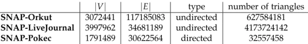
5 Methodology 25 5.1 Network data . . . . 25

5.2 Hardware and software platform . . . . 25

5.3 Measurements . . . . 26

6 Evaluation of shared memory and distributed LCC 27 6.1 Local LCC computation . . . . 27

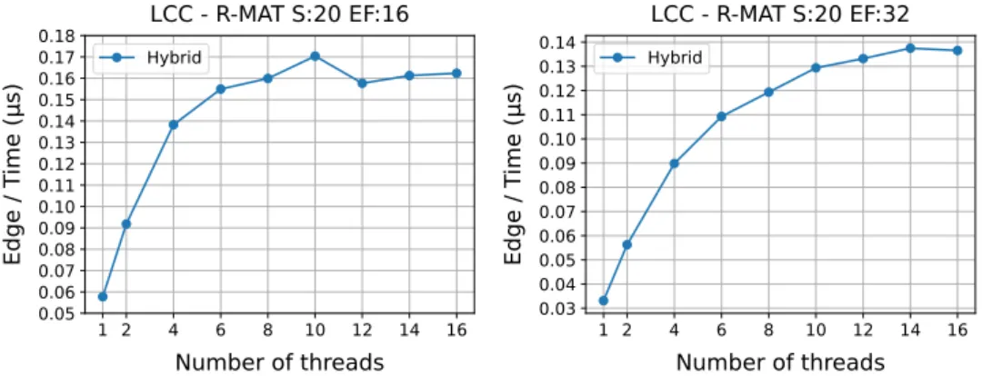
6.1.1 Performance of the hybrid method . . . . 27

6.1.2 Scaling . . . . 28

6.2 Distributed LCC . . . . 29

6.2.1 Caching performance . . . . 29

6.2.2 Overall performance . . . . 32

6.3 Summary and lessons learned . . . . 33

6.4 Future directions . . . . 34

6.4.1 Vectorization . . . . 34

6.4.2 Node level caching . . . . 34

Bibliography 35

Chapter 1

Introduction

With the emergence of the Internet, in various contexts entities have been connected resulting in different types of networks. The WWW itself forms a network where entities are the web pages that are connected together by hyperlinks. Taking E-mails as an example, by sending a message a link between the sender and the receiver is created. Thus, by collecting the mes- sages between a group of users we arrive at a communication network. An- other example is social networks, such as Facebook or Twitter where links between the users often represent friendship or some kind of interest to- wards the other user.

The analysis of such networks can be of benefit in many ways. Facebook, for example, might achieve a better quality of service by understanding the main drivers in creating new connections. The analysis of E-mail traffic can help for better spam filtering or in the detection of fraud. Network analysis has an important social aspect as well, as better understanding of the structure of our society will also help us identifying and supporting minorities.

While all the networks described above represent different relationships, they all share the property of consisting millions or even billions of enti- ties. Therefore, the analysis of these networks has a higher demand both in memory and computing capacity than today’s single CPU machines can offer. This leads to the necessity of the development of distributed solutions.

Lumsdaine et al. [14] point out several properties of graph problems that make it difficult to develop distributed programs with good performance.

Firstly, most graph analytical problems are data-driven, that is the computa-

tion depends on the underlying structure of the graph. However, it is often

not known before execution, what makes it difficult to evenly partition the

problem among the computing nodes. Secondly, the data access of such

problems has often poor locality that comes from the irregular and unstruc-

1.1. Notation

Graph structur e

G a given graph, G = ( V, E ) ; V, E are sets of vertices and edges.

n, m numbers of vertices and edges in G; n = | V | , m = | E | . deg ( i ) degree (out-degree) of i.

adj ( i ) adjacency of vertex i.

A adjacency matrix of G.

4

a triangle including the edges e

, e

, e

∈ E i − j − k two path including e

, e

∈ E.

Table 1.1: Symbols used in the thesis; i, j, k ∈ V are vertices.

tured relationships in the data. Finally, graph analytical problems tend to be communication-heavy because they need to explore certain regions of the graph but do less computation on the graph data.

1.1 Notation

We denote an unweighted graph that contains no multi-edges and loops as G = ( V, E ) , where V is the set of vertices and E ⊆ V × V the set of edges.

We will use i to denote the vertex v

∈ V and e

for the edge between i and j.

For undirected graphs it holds that e

= e

. We set | V | = n and | E | = m. We can define the adjacency of i as adj ( i ) = { v

: e

∈ E } and the degree of i as deg ( i ) = | adj ( i )| (Note, for a directed graph, this regards to the out-degree of a vertex). We will refer by i − j − k to the two path from i to k containing the edges e

and e

. To denote a triangle consisting of vertices i,j,k and the edges e

, e

and e

we use the symbol 4

.

1.2 The Local Clustering Coefficient

The Local Clustering Coefficient (LCC) of a vertex i was defined by Watts and Storngratz [19] as the proportion of existing edges between the vertices adjacent to i divided by the possible number of edges that can exist between them.

Definition 1.1 (Local Clustering Coefficient) For a directed graph G the local clustering coefficient of a vertex i is defined as:

C ( i ) = |{ e

: v

, v

∈ adj ( i ) , e

∈ E }|

deg ( i ) ∗ ( deg ( i ) − 1 ) Similarly, for an undirected graph:

C ( i ) = ² ∗ |{ e

: v

, v

∈ adj ( i ) , e

∈ E }|

deg ( i ) ∗ ( deg ( i ) − 1 )

1.3. On the difficulty of triangle computation We can see that for a pair of vertices { j, k } , in order to contribute to the numerator, the edges e

, e

and e

must exist. This means that they form the triangle 4

in G. Thus, if the degrees of the vertices are known and a found triangle can be assigned to the corresponding vertex, triangle counting and the computation of the local clustering coefficient can be regarded as the same problem. In the following, we will use the shorthand LCC for the local clustering coefficient and TC for triangle counting.

1.2.1 Significance of Triangles and LCC

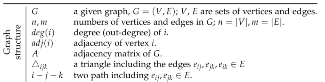
Already in 1988, Coleman [5] argued that the existence of triangles (closure, as he calls it) is a necessary condition for the emergence of norms in societies.

He illustrates it with the simplest example, shown in Figure 1.1. If actors B and C are not connected to actor A, it may be able to negatively influence both B and C, without they had alone the power to resist. However, if there is some connection between them, collectively they may be able to sanction A, or one could reward the other for doing so. In that case, closure would stop the propagation of A’s negative influence in the network.

The LCC was found useful in numerous applications as well, such as for community detection in networks, database query optimization, or link clas- sification and recommendation. For example, Becchetti et al. [3] show that both the number of triangles and the local clustering coefficient are good measures for separating web spams from non-spam hosts. Remarkably, in the dataset they inspected, the approximated LCC was found to be the 14th best indicator for spams out of over two hundred properties.

Figure 1.1: A society with (a) and without (b) closure. Figure from [5].

1.3 On the difficulty of triangle computation

In the following, we assume that the graph is stored in a form that sup-

ports constant-time edge queries. Any graph G can have at most O( n

)

triangles. This is the case when there is an edge between every vertex of G,

making it an n-clique. This inherently sets the worst-case running time of

1.3. On the difficulty of triangle computation any algorithm for TC at O( n

) . We can distinguish the following two basic approaches for triangle counting:

Algorithm 1: Vertex based Triangle Counting Result: The number of triangles in G stored in counter

1:

counter = 0

for all i ∈ V do

for all j ∈ V do

for all k ∈ V do

5:

if ( i, j ) , ( i, k ) , ( j, k ) ∈ E then

6:

counter += 1;

7:

end if

8:

end for

end for

end for

11:

return counter;

Algorithm 2: Edge based Triangle Counting

Result: The number of triangles in G stored in counter

counter = 0

2:

for all i ∈ V do

3:

for all pair of distinct j, k ∈ adj ( i ) do

if ( i, j ) , ( i, k ) , ( j, k ) ∈ E then

counter += 1;

6:

end if

end for

end for

9:

return counter;

Vertex-centric. Trivially, one can find every triangle in a graph by enumer- ating the overall triplet of vertices and check whether edges exist between them. This approach is showed in Algorithm 1. This simple method leads to a Θ ( n

) running time.

Edge-centric. Shifting our focus from vertices to edges, we can solve TC by enumerating over every two-paths. The pseudo-code of this approach is shown in Algorithm 2. We do Θ ( _deg ( _i )

) work for every vertex, resulting in a overall running time of Θ ( _∑

deg ( i )

) .

Whereas the vertex-centric approach depends only on the number of vertices

in G, the running time of the edge-centric algorithm is dependent on the

structure of the graph. For example, if every vertex has a constant degree,

vertex-based TC would still have a time complexity of Θ ( n

) but an edge-

based algorithm would run in Θ ( n ) . We note that for a graph with a highly

1.4. Overview of the thesis skewed degree distribution a basic edge-based algorithm would spend most of the work at vertices with the highest degree, even though many of its neighbors may have degree one and thus they can not be part of a triangle.

For an extreme example, one can consider a star-graph for which the edge- centric algorithm is in Θ ( n

) , but it has zero triangles. This shows how pre-processing the graph can have a significant effect on the running time.

1.4 Overview of the thesis

In this thesis we particularly focus on real-world graphs. Such networks have a power law degree distribution, that means that the fraction of P ( k ) nodes having degree k is:

P ( k ) ∼ k

typically for 2 < α < 3. Its main implication for our purpose is the emer- gence of hubs in such networks, that is, the network will have a small num- ber of nodes having a degree multiple orders of magnitude bigger than the rest of the network.

The focus of this thesis is two-fold. Firstly, we analyse different methods used for triangle computation and develop a hybrid method to achieve bet- ter performance on shared memory. We take advantage of OpenMP [6]

for shared memory parallelism on edge level. Secondly, we analyze our distributed program for triangle counting that relies on a 1-dimensional partitioning scheme of the vertices. For the communication between the computing nodes, we take advantage of MPI’s Remote Memory Access [10]

interface. We use CLaMPI [7], a software cache for remote memory access.

We analyze how CLaMPI’s design choices and the graph structure affect the

caching performance and thus, the overall communication time.

Chapter 2

Related works

In the following, we give an overview of the different techniques used for distributed triangle counting. Instead of discussing related papers in detail, we focus on the two main parts of TC, namely the computation of triangles and the partitioning of the graph.

2.1 Computation of triangles

2.1.1 Frontier intersection

One way to compute the triangles is by intersecting the adjacency lists of every pair of vertices i, j for which e

∈ E. We will use A and B to denote the adjacency lists of i and j respectively.

Naive intersection. In case the adjacency lists are not sorted, a naive way to compute A ∩ B would be to compare every element in A with every element in B resulting in a running time of O(| A | ∗ | B |) .

Hashing. Still without sorting, one can utilize hashing to reduce the compu- tation time. Using one of the lists a hash table can be built with the help of some adequately chosen hash function. The computation of the intersection is then achieved by hashing every element from the other list and checking whether a match exists. The method’s main advantage is that the hash table built from the adjacency of vertex i can be reused for the intersection with every other vertex j ∈ adj ( i ) . However, there is extra place necessary for storing the hash table which can be a bottleneck for big graphs. Moreover, the handling of collisions in the hash table is another key part, which can also be time-consuming.

Pandey et al. [16] utilize hashing, but instead of hashing every element, they

use a certain number of bins in which they store multiple elements. An

2.1. Computation of triangles Algorithm 3: Sorted set intersection for A ∩ B

Result: The number of common elements in A and B

counter = 0

2:

i, j = ₀

3:

while i < length ( A ) _and j < length ( B ) _do

if A [ i ] == B [ j ] _then

5:

counter += 1;

6:

i += 1;

j += 1;

7:

else if A [ i ] < B [ j ] then

8:

i += 1;

9:

else

10:

j += 1;

11:

end if

end while

return counter;

element j ∈ B is then first hashed into one of the bins and then compared to every element belonging to that bin using linear search.

For the following two algorithms we assume that the neighborhood lists are sorted in increasing order.

Sorted set intersection (SSI). We can traverse the two lists simultaneously by comparing the current elements and progressing in the array whose cur- rent element is smaller. The pseudo-code of SSI is given in Algorithm 3.

Trivially, SSI computes the intersection of two lists in O(| A | + | B |) .

Binary search. Alternatively, the intersection of two lists can be seen as locating every element from one list in the other one. Thus, the problem becomes doing | A | lookups in a sorted array of length | B | , which can be done in O(| A | ∗ log (| B |)) by using binary search. The algorithm is outlined in Algorithm 4. To minimize the time complexity one should always assign the longer list as the search tree and the shorter one as the array of keys.

This method was first introduced by Hu et.al. [11].

By comparing the running times of the binary search-based and sorted set intersection-based algorithms, we see that SSI is faster if:

p + q ≤ p ∗ log

( q ) (2.1)

q ≤ p ∗ ( log

( q ) − 1 ) (2.2) q

p ≤ log

( q ) − 1 (2.3)

As our focus is on graphs with highly skewed degree distribution, we would

expect that

is big for most of the edges, favoring the binary search method.

2.1. Computation of triangles Algorithm 4: Binary search for A ∩ B

Result: The number of common elements in A and B

Assuming length ( A ) < length ( B )

2:

counter = 0

3:

bottom = 0 top = length ( B ) − 1

for all x ∈ A do

5:

while bottom < top − 1 do

mid = b( top − bottom ) _/2 c

if x < B [ mid ] _then

8:

top = mid;

9:

else if x > B [ mid ] then

bottom = mid;

11:

else

12:

counter += 1;

13:

break

14:

end if

end while

end for

17:

return counter;

We emphasize that the two methods above assume sorted adjacency lists.

Even though, with many data sets, this is given for free, this overhead has to be taken into account when comparing these algorithms with others.

2.1.2 Algebraic computation

We describe the following method for an undirected graph G, but it can be extended to directed graphs as well. The adjacency matrix A of G can be written as the sum of the lower and upper triangular matrix L and U. The entries of L represent all the edges e

∈ E for which i < j and similarly U stores the edges e

∈ E, such that j < i. Therefore, by computing B = _LU the matrix B will store every two-paths i − j − k for which i < j < k. Such two paths are closed into a triangle if the edge e

∈ E. Therefore, to obtain every triangle in G we can compute C = A ◦ B (Hadamard product). To attain the LCC for node i one can sum the values of the ith row of C and then divide it by the degree of the vertices.

TC implementations based on the algebraic computation method take ad- vantage of the sparsity of G and use highly-optimized libraries for sparse matrix multiplication. A parallel implementation with further improve- ments can be found in the paper from Azad and Buluc¸ [1], and a distributed algebraic-based TC algorithm has been implemented by Hutchinson [12] us- ing the Apache Accumulo distributed database.

Aznaveh et al. [2] implemented shared memory parallel TC and LCC com-

putation based on the SuiteSparse GraphBLAS implementation of the Graph-

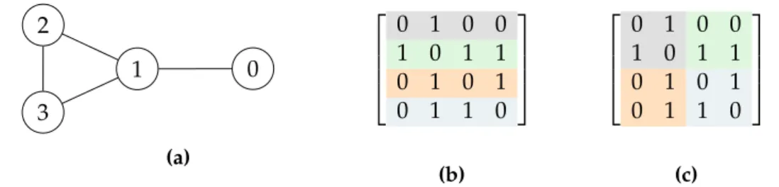
2.2. Graph partitioning

0 1

2

3

(a)









0 1 0 0 1 0 1 1 0 1 0 1 0 1 1 0









(b)









0 1 0 0 1 0 1 1 0 1 0 1 0 1 1 0









(c)

Figure 2.1: An example graph (a) and its basic 1D (b) and 2D (c) partitioning BLAS standard. The implementation uses OpenMP to achieve multithread- ing. They follow the algebraic method as well and compute the product of the upper and lower triangular matrix of the adjacency matrix with sparse matrix multiplication. For the LCC additional work is necessary to attain the degree of the vertices which leads to a significantly lower speedup com- pared to TC.

2.2 Graph partitioning

In the following, we discuss several techniques to achieve distributed TC.

We note that both the time spent with communication and computation can depend on the partitioning scheme. We assume that there are p computing nodes available P

, P

, . . . , P

, p = 2

for some k and p divides n.

2.2.1 1D partitioning

One dimensional partitioning assigns equal sized blocks of vertices to nodes, that is we partition V into p distinct sets V = V

∪ V

. . . ∪ V

. A basic 1D partitioning can be achieved by:

V

=

v

: i ∈

( k − 1 ) ∗ p n , k ∗ p

n

The node that owns vertex i will own every edge starting from i, and it will compute the LCC of i.

Whereas 1D partitioning can be done without pre-processing and introduces no space overhead, it suffers from the in-equal distribution of edges if G has a highly-skewed degree distribution. To partially overcome this one can sort the vertices by degree and instead of a block-based distribution cyclically distribute the vertices among the computing nodes.

2.2.2 2D partitioning

Two dimensional partitioning assigns edges to processes in a grid based

manner, partitioning the adjacency matrix A into a grid with dimensions

2.2. Graph partitioning

√ p × √

p such that E = E

∪ E

. . . ∪ E

∪ . . . E

. The basic 2D partitioning of a graph is given by:

E

=

e

: i ∈

( u − 1 ) ∗ √ p n , u ∗ √

p n

∧ j ∈

( v − 1 ) ∗ √ p n , v ∗ √

p n

The difference between 1D and 2D partitioning is visualized in Figure 2.1. To intersect the neighborhood lists of nodes i and j one has to first gather them issuing √

p − 1 vertical and horizontal communications with other processes.

To overcome this communication overhead, Tom and Karpys [18] developed a TC algorithm for undirected graphs following a parallel matrix multipli- cation scheme. They solve TC by computing a matrix C whose entry c

stores the number of triangles that contain e

. This can be computed by c

= U

L

if the triangles are ordered by i < j < k. However, a process P

only stores the parts L

and U

. Therefore, it firsts multiplies its local blocks and then shifts L left by one along its row in the processor grid and U up by one along its column. After √

p local multiplies and shifts the desired entry is computed.

2.2.3 Partitioning with proxy vertices

To completely avoid communication every process can store additional proxy

vertices and corresponding edges that are necessary for computing triangles

locally. This method was introduced for TC by Hoang et al. [8] who split

the partitioning of the graph into 3 steps. First, every vertex gets assigned

to a process by a 1D partitioning scheme. Then proxy vertices are created

for every edge whose endpoint does not belong to the same process as its

starting point. Finally, the newly added proxy edges are connected. We note

that care has to be taken in order not to count a triangle multiple times.

Chapter 3

MPI-RMA and Caching

3.1 MPI-RMA

For communication between processes, we take advantage of MPI’s Remote Memory Access programming environment [10]. MPI-RMA allows pro- cesses to directly read from or write to non-local memory regions using remote direct memory access (RDMA). RDMA is implemented in hardware and can bypass the operating system allowing faster communication with lower CPU usage than other communication methods.

In MPI-RMA processes are organized into communication groups in which the participants can expose a certain region of their local memory through the creation of a window. Processes may allocate a new memory region to be shared in the window, attach an already allocated region or establish a win- dow without an underlying memory buffer and subsequently bind regions to it. Furthermore, MPI-RMA allows processes to share a buffer attached to a window between multiple processes by shared window allocation. This can be useful for multicore nodes where MPI processes on the same node share memory. Remote accesses to a window are always addressed relative to the start of the window at the target process.

Once a window is established, processes can read from or write to this

now shared memory region. The two basic operations for data movement

are MPI Get and MPI Put for the reading and writing of non-local mem-

ory. Furthermore, additional atomic operations are defined to accumu-

late data. The MPI CAS function can be used for remote atomic com-

pare and swap operation and MPI Accumulate for updating data by com-

bining the existing remote data and the data sent with the accumulator. The

MPI GetAccumulate allows remote read-modify-write operations. A simpler

version of MPI GetAccumulate is MPI FetchAndOp that limits the data to a

single element in order to allow hardware optimizations and thus achieve

faster completion.

3.2. Caching Communication in MPI-RMA is always non-blocking and is split into epochs that are started and ended by synchronization. The process-local mem- ory region can be accessed by other processes during an exposure epoch, whereas a process can access remote data during an access epoch. Processes may be simultaneously in an access and exposure epoch. Epochs form a unit of communication and all communication operations are completed at epoch closure.

There are two methods to achieve synchronization between processes based on whether the target process is involved in synchronization. In active target synchronization, a process exposes its memory region for an epoch, during which it can allow either only read or both read and write operations. Fine- grained synchronization can be achieved by allowing processes to decide for which other processes they open an access or exposure epoch. On the other hand, with fence synchronization, all processes synchronously call fence to start or end an epoch. With passive target synchronization processes always make their memory available either to processes that specifically locked it or globally to all processes in the communicator. In the single-process lock- /unlock model acquiring a lock guarantees local memory consistency and releasing the lock closes the epoch and guarantees remote memory consis- tency.

3.2 Caching

A cache is a small storage that aims at speeding up the access of instructions or data by storing frequently used elements. Caches can be implemented in hardware, such as CPU or GPU caches, or in software such as Web caches.

Data caches became very important in recent years as the rate of improve- ment in processors exceeded the rate of improvement in storage and data bus technologies. Thus, data movement became a bottleneck in computa- tion making the need for a hierarchical storage structure that stores a small set of regularly accessed data ”closer” to the CPU. In the case of hardware caches, this is achieved by different technologies used for caches than for main memory which supports faster data access. A software cache reduces data movement by storing a subset of the commonly accessed data locally thus saving remote communication.

3.2.1 Locality

Caches are based on the locality principle which says that programs tend to access either the same data multiple times or elements close to the previ- ously accessed ones.

Temporal locality. Data that has been recently accessed is likely to be ac-

cessed in the near future as well. Examples of this are variables that are

3.2. Caching frequently used in a program (e.g. counters, or some constant).

Spatial locality. Nearby elements are often accessed close together in time.

When traversing an array a program sequentially loads the elements from memory. Thus, if we cache some elements beforehand we can reduce the number of memory accesses and increase performance.

3.2.2 Hitting and missing

We call the set of data elements referenced by a program during a time period [ t − τ, t ] the working set, denoted by W ( t, τ ) . A cache hit occurs if the accessed element was present in the cache. Otherwise, we have a cache miss and the element has to be transferred from some other storage unit. In case of a miss, an old entry, called the victim, may need to be evicted in order to make space for the new element. This is called the eviction procedure and is crucial for good cache performance. Cache misses can be classified into three groups:

Compulsory misses. Every element in the working set has to be loaded into the cache first, resulting in a compulsory cache miss.

Capacity misses. If the working set of a program is bigger than the size of the cache, there will be no space left for some elements, causing capacity misses. The number of capacity misses can be reduced by increasing the cache size, or by a better eviction strategy.

Conflicting misses. Every element in the cache has to have an address to be accessible. If two elements from the working set map to the same address, they will produce a conflicting miss. Conflicting misses can be also reduced by the eviction strategy, or by the structure of the cache. For example, by using a fully associative cache, i.e. we store every entry under the same address in an array, we can fully eliminate conflicting misses, for the prize of longer lookup times. For hardware caches, increasing the cache size can also reduce the number of conflicting misses.

3.2.3 CLaMPI

CLaMPI [7] is a caching layer for remote memory access. It is built on top of

the MPI-RMA programming environment with the intention to fit into MPI’s

semantics thus enabling caching with minimal code changes necessary from

the user. ClaMPI stores remote memory reads (called a get operation in

MPI-RMA) that return the desired part of an exposed memory region from

another process inside the communication group. CLaMPI handles variable-

sized entries to flexibly support such read operations. In the following, we

discuss its most important design choices that will be useful for the analysis

of its performance for triangle counting.

3.2. Caching 3.2.4 Structure of CLaMPI

CLaMPI implements a caching layer using two data structures, a hash table to index the entries and an AVL tree to store the free regions in the under- lying memory allocated for the cache. For a cache C

that stores gets issued on the window w, we denote the corresponding hash table by I

and the size of the memory reserved by S

.

A get targeting a caching enabled window w is first hashed to check whether it is present in the cache. To minimize hash collisions four hash functions h

. . . h

are used that are randomly selected until either the entry is found in the cache (cache hit) or a free space in the index is found. A conflicting miss occurs if for an entry e no empty index is found with any of the hash functions.

For the entries in the cache a contiguous memory of size S

is allocated. S

should be a multiple of the CPU’s cache line size. The AVL tree used for storing free regions serves free region queries in O( logN ) time, where N is the number of free regions. Furthermore, it provides a best fit policy for the allocation of new entries. Nonetheless, due to the contiguous memory layout, after several evictions, the storage may get fragmented. This can lead to capacity misses even if there is altogether enough memory to serve an insertion.

3.2.5 Handling of cache misses

As CLaMPI caches remote memory reads at the moment of issuing the re- mote read, the data targeted by the read is not yet available. However, a corresponding entry is allocated in the cache, therefore an entry’s state is not either missing or cached but can be pending. Pending is an intermediate state meaning that it has been successfully indexed as well as a suitable space has been reserved for it but the data has not arrived yet. An entry transfers from pending to cached at epoch closure.

Compulsory misses. A compulsory miss means that the data was not found in the cache, however, there has been a free entry found in I

as well as a space big enough to store the data. The entry’s state always becomes pending.

Conflicting misses. In case of a conflicting miss there is enough space to store the data but all h

( e ) . . . h

( e ) led to a collision in the hash table. A victim is chosen randomly out of these four entries and evicted. Therefore, similarly to a compulsory miss, an entry’s state always becomes pending after a conflicting miss.

Capacity misses. A capacity miss means that there is no free region big

enough to store the data, therefore a victim has to be selected. CLaMPI

3.2. Caching does not guarantee insertion in case of a capacity miss but always evicts one entry. This is because multiple evictions may be necessary to make a space big enough for the entry. This could lead to a significant overhead.

Furthermore, if the entry is a highly accessed one, after several evictions enough space may be freed to cache. As a result, after a capacity miss the element may stay in missing status.

For the handling of capacity misses the following algorithm is used to choose a victim entry to evict. First, an interval I

[ i : i + α ] in the hash table is se- lected randomly, where the length of the interval α can be set by the user.

Assuming that the entries in the hash table are uniformly distributed (which is a corollary of the hash function used) this interval represents a random sample of entries.

A score R is assigned to every entry at insertion which is then used for selecting the victim. R is computed by the entries temporal score R

and positional score R

, R = R

∗ R

. The score of an entry seeks to maximize the caching performance by representing an entry’s probability to be used in the future as well as counteracting fragmentation in the memory allocated for the cache.

The temporal score follows a least recently used scheme and is computed by R

=

numbef of gets issued in the window

. The positional score assigns a lower value to entries that have bigger free spaces adjacent to them. On the one hand, this reduces fragmentation. On the other hand, by evicting an entry with a lower positional score, it is more likely that enough space will be freed up to store the new entry. Let ¯ s

be the average size of entries present in the cache after the i-th get and q

the size of free memory adjacent to the entry e. The positional score of an entry e after i gets is then given by:

R

( e ) = min

| s ¯

− q

|

¯ s

, 1

3.2.6 Adaptive scheme

CLaMPI’s performance is highly dependent on the size of memory allocated for the cache and on the configuration of the index table. In the context of caching remote memory accesses, the working set W ( t, τ ) can be viewed as the set of gets issued in the time interval [ t − τ, t ] . Denoting the set of cached entries at time t that belong to the working set by γ ( t, τ ) we have the following two constraints:

| γ ( t, τ ) ≤ | I

| and ∑

g∈γ(t,τ)

size ( g ) ≤ | S

|

3.2. Caching As for the memory size, while it is beneficial to increase S

if the total size of gets exceeds the total capacities of the machine, one has to bound S

in order not to run out of memory.

The size of the hash table (index size) also influences the caching perfor- mance as well as the overhead of CLaMPI. In case when | I

| is too small the number of conflicting misses will get large, thus constantly evicting entries leading to a bad utilization of the cache memory. On the other hand, if | I

| is too big, the random set selected for eviction after a capacity miss may be empty. As CLaMPI always evicts an entry, this would lead to traversing more than α elements and thus increasing the overhead.

As finding the correct settings for I

and S

can be cumbersome, CLaMPI offers an adaptive mode that dynamically adjusts them. A sign for a too small I

is when the portion

total gets

exceeds some bound. A too big I

can be detected based on the number of empty entries traversed at eviction

after a capacity miss. While it is important to have a hash table and memory

size suitable to the program, as changing any of the parameters requires the

invalidation of the cache, caching performance may be decreased due to the

numerous flushes.

Chapter 4

Distributed LCC with CLaMPI

In the following, we outline our distributed implementation for the com- putation of the local clustering coefficient and discuss how caching can be done in order to reduce communication.

4.1 Outline of our implementation

4.1.1 Graph pre-processing and distribution

We start by reading in the edge list of the graph from external storage in parallel. As a second preparation step, we remove every loops and multi- edges in the graph.

As we hope that caching can significantly reduce communication we min- imize the overhead of pre-processing and partitioning. By this reason, we use 1D partitioning to distribute the graph and after partitioning the only pre-processing applied is the removal of vertices that have a degree less than two. It is easy to see that such vertices cannot be part of a triangle.

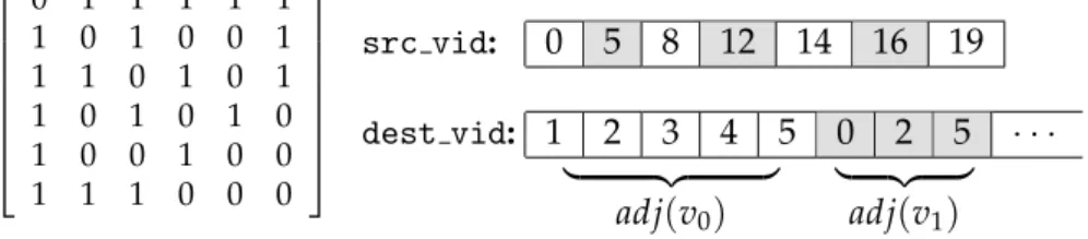
4.1.2 Graph format

We convert the edge list of the graph into a compressed sparse row (CSR)

format. CSR stores a binary matrix using two arrays that we call src vid and

dest vid. For a graph G the pair of entries src vid[i], src vid[i+1] store

the beginning and the end of the adjacency list of the vertex i. Respectively,

the slice dest vid[src vid[i]:src vid[i+1]] stores the adjacency of the

vertex i. Note that the out-degree of a vertex i is thus given by deg[i] =

row[i+1] - row[i].

4.1. Outline of our implementation

















0 1 1 1 1 1

1 0 1 0 0 1

1 1 0 1 0 1

1 0 1 0 1 0

1 0 0 1 0 0

1 1 1 0 0 0

















src vid: 0 5 8 12 14 16 19 dest vid: 1 2 3 4 5 0 2 5 · · ·

| {z } | {z } adj ( v

) adj ( v

)

Figure 4.1: A graph represented by its adjacency matrix and the correspond- ing CSR representation.

4.1.3 Communication

We use MPI’s One Sided interface to read non-local partitions of the graph by creating two communication windows w

and w

in which processes share its local src vid and dest vid arrays. Both windows are created with a communication group containing every process. We follow the passive target synchronization method as the graph is never changed hence there is no synchronization necessary. At the beginning of the computation, we globally lock both windows and unlock them only when every process is finished. As a result, the processing of vertices is fully asynchronous.

By distributing the graph among multiple processes, source vertex IDs be- come local in the CSR representation. We denote by n the number of vertices in G and by p the number of computing nodes used. In order to determine which process owns a vertex, and what is its local ID we can use the follow- ing rules:

Local ID to global ID: global ID = local ID * (n / p) + local ID Global ID to local ID: local ID = global ID / (n / p)

Process ID: dest proc = global ID % (n / p) 4.1.4 Triangle computation

Every process computes the LCC score of all the vertices it owns one after the other, to achieve locality. We follow the edge-centric way of TC and count the number of triangles of which vertex i is part of by computing adj ( i ) ∩ adj ( j ) for every j ∈ adj ( i ) . We achieve shared memory parallelism by doing the computation of the intersection in parallel, for which we used OpenMP.

4.1.5 Implemented algorithm

The outline of the final algorithm is depicted in Algorithm 5. Lines 1-5

represent the reading, pre-processing and 1D distribution of the graph. In

4.1. Outline of our implementation

line 7 the graph is already distributed, and thus the communication epoch

for both windows w

and w

can be started. In the case of an edge having an

endpoint that belongs to a different process, the remote read of its degree

and adjacency list happens in Lines 17-18. We note that the remote read

targeting w

is dependent on the read targeting w

as src vid[i] stores

the address of the adjacency list of the vertex i in dest vid. Lines 24-36

compute the intersection, where we dynamically assign the lists based on

their lengths, as well as choose the method used for the intersection. In Line

40 the computation of LCC of every local vertex has been finished.

4.1. Outline of our implementation Algorithm 5: Distributed LCC computation

Result: Local clustering coefficient for every local vertex.

1:

edge list ← ReadInGraph(G);

2:

edge list ← NormalizeGraph(edge list);

3:

edge list ← 1DPartitioning( edge list );

4:

src vid , dest vid ← BuildCSR( edge list );

5:

local verts = n / p ;

lcc[] ;

7:

MPILockAll() // Start the communication epoch for all processes.

8:

for v src in 0 . . . local verts-1 do

9:

src degree = src vid[i+1] - src vid[i] ;

10:

src adjacency list = dest vid[src vid[i]:src vid[i+1]-1];

11:

triangle count = 0;

12:

for all v dest in src adjacency list do

dest processID = b v dest / local verts c ;

v dest local = v dest % local verts;

15:

// If the endpoint of the edge is non-local, it has to be attained.

16:

if dest processID ! = myID then

17:

dest degree ← RemoteRead(dest processID, v dest, src window);

18:

dest adjacency ← RemoteRead( dest processID , v dest , dest window );

19:

else

20:

dest degree = src vid[v dest local+1] - src vid[v dest local] ;

dest adjacency list =

dest vid[src vid[v dest local]:src vid[v dest local+1]-1] ;

end if

23:

// Prepare for intersection.

24:

if length(dest adjacency list) < length(src adjacency list) then

shorter list = dest adjacency list;

26:

longer list = src adjacency list;

27:

else

28:

shorter list = src adjacency list;

29:

longer list = dest adjacency list;

30:

end if

31:

// Decide which method to use for intersection. The intersection is done in parallel.

32:

if DecideIntersection( shorter list , longer list ) then

33:

triangle cnt += SortedSetIntersection( shorter list , longer list );

34:

else

35:

triangle cnt += BinarySearchIntersection( shorter list , longer list );

36:

end if

end for

38:

lcc[i] = ComputeLCC(triangle cnt, src degree)

end for

40:

MPIUnlockAll() //Close the communication epoch for all processes

return lcc;

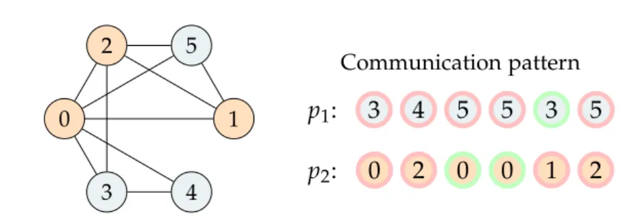
4.2. Caching for distributed LCC

0 1

2

3 4

5 Communication pattern

p

: 3 4 5 5 3 5 p

: 0 2 0 0 1 2

Figure 4.2: (Left) The graph from Figure 4.1 partitioned with 1D partitioning among two processes. (Right) The sequence of remote accesses, with green showing cache hits.

4.2 Caching for distributed LCC

In case multiple local vertices have a common non-local neighbor, the same data has to be transferred several times. In order to decrease communication one can introduce caching to store, next to the own vertices, some of the most often accessed non-local vertices as well. This approach is most similar to the proxy vertices method discussed in Section 2.2.3. The entries in the cache can be regarded as a dynamically determined sub-graph containing vertices that have been accessed regularly and thus are expected to be accessed in the future as well.

4.2.1 A small scale example

To illustrate how caching can reduce communication, consider the scenario depicted in Figure 4.2. We partitioned the graph using 1D partitioning among two processes p

(blue) and p

(orange). If no caching is used 12 times the neighborhood list of a non-local vertex is read by either of the processes.

Now suppose we operate with a cache layer that can store the adjacency of one vertex, and after an entry was inserted into the cache it does not get evicted. Assuming we process the vertices in increasing order, p

would cache the neighborhood list of v

and p

of v

. This would result in 3 cache hits leading to a reduction in communication by 25%. We have 3 capacity misses and 5 compulsory misses limiting the best achievable improvement to 42%.

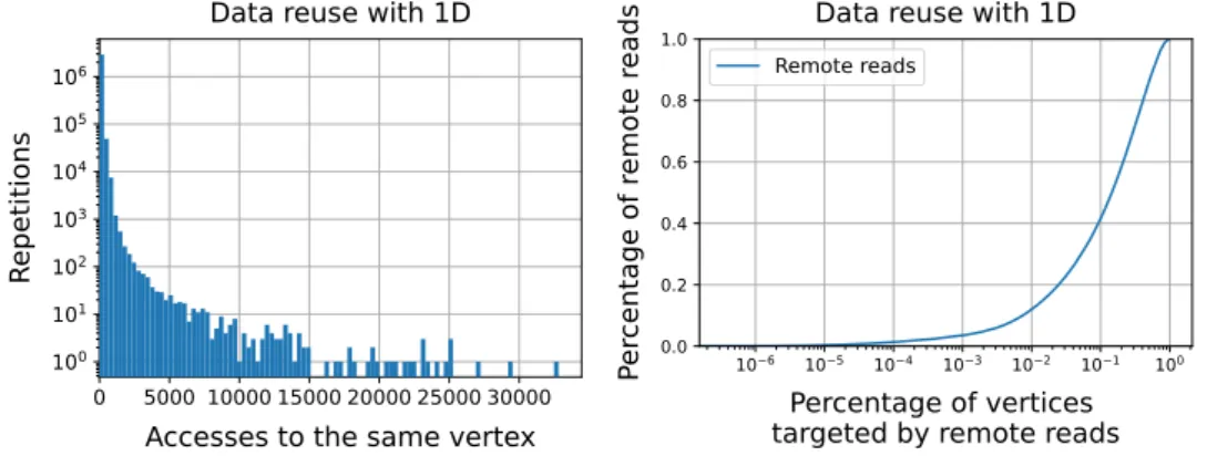
4.2.2 A large scale example

In general, by distributing the graph among several processes a high por- tion of the edges will have endpoints belonging to different partitions. For example, for a graph with 2

vertices and 2

edges partitioned into 4 parti- tions by the 1D method 95% of the edges go between two distinct partitions.

Therefore, communication may become dominant in LCC computation. Fur-

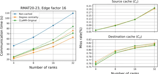
4.2. Caching for distributed LCC thermore, as most real-world networks follow a power law, a big portion of the remote reads will target the same vertices. Figure 4.3 shows how the highest degree nodes contribute to the number of remote accesses and to the total data transferred between processes. We can see that only 10% of the highest degree vertices make up more than 40% of the number of remote reads.

Figure 4.3: Data reuse for the SNAP-LiveJournal graph. (Detailed in Table 5.1)

4.2.3 CLaMPI for distributed LCC

As discussed earlier, we use CLaMPI to cache remote reads. The caching happens at lines 17 and 18 in Algorithm 5. We enable caching for both windows, that is we have a cache layer C

for src vid and C

for dest vid at every process. We denote the sizes of the arrays of a graph’s CSR rep- resentation by | src vid | and | dest vid | . Moreover, we use | src vid |

and

| dest vid |

for parts locally stored at the process p

. 4.2.4 Configuration of CLaMPI

Assuming that vertices are assigned randomly to computing nodes, the in- degree of a vertex explicitly correlates with the number of times it will be remotely accessed. Using p computing nodes, a node p

will access a non- local vertex j in expectation

times. Therefore, if caching is done properly, we expect to store some of the highest in-degree nodes.

For the configuration of C

this has no special implications as src vid stores

only the location of the adjacency arrays. Thus, for every vertex indepen-

dently from its degree, the corresponding cache entry will have a size of

two.

4.2. Caching for distributed LCC However, C

is closely dependent on this observation. As we focus on scale- free graphs, the difference between degrees is huge and a small percent of the vertices is expected to be adjacent to most of the edges.

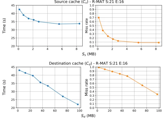
Cache size. While the bigger the cache is the better performance we could achieve, we have to limit the cache size in order to simulate a scenario where memory becomes a bottleneck. As C

depends only on the number of ver- tices, we can tune it so that we achieve a relatively low miss rate. On the other hand, S

depends on the number of edges in the graph, therefore its size has to be more limited.

Index size. To set the index size we have to estimate the number of entries we expect to store in a cache with a given size. For C

this is I

= S

/2, as every entry will have a size of two.

We first describe the rule for setting the index size of C

for undirected graphs in which case in-degree equals out-degree. Let the size of C

be S

and denote the total size of the non local adjacency lists for a process p

by d

( d

= | dest vid | − | dest vid |

). To get a good approximation we will use that the underlying graph is a power law graph, that is the fraction of p ( k ) vertices having degree k can be well approximated by p ( k ) = C ∗ k

for some constant C, and 2 < α < 3.

Assume that k is a continuous real variable following a power law p ( k ) . We are interested only in the case where 2 < α. As p ( k ) represents a probability distribution, we can compute C as:

1 =

Z

kmin

p ( x ) dx ⇒ C = R

¹

kmin

x

dx = ( ₁ − α ) [ x

]

min

= ( α − 1 ) ∗ k

(4.1) Keeping the assumption that the graph’s degree distribution is approxi- mated by a continuous power law p ( k ) , the fraction of vertices that have degree bigger than k is given by:

p ( k ) =

Z

k

P ( x ) dx = C ∗

Z

k

x

dx = ^C

α − 1 k

= k

k

(4.2) Furthermore, we can compute the fraction that such vertices make up out of the sum of all degrees (e.g out of | dest vid | ) as:

W ( k ) = R

k

x

dx R

kmin

x

dx = k

k

(4.3)

By re-organizing both to eliminate

min

we get that the fraction W of the sum of the degrees of P of the highest degree vertices is:

W = P

(4.4)

4.2. Caching for distributed LCC Going back to our initial problem, that is determining a suitable index size, we have that process p

can store P = S

/d

percent of the non-local adja- cency lists in the cache. By using (4.4) we get that this portion corresponds to W = ( S

/d

)

fraction of the highest degree vertices. Therefore, we set the index size to | I

| = n ∗ ( S

/d

)

.

This method is clearly an approximation, as neither does a graph’s degree distribution strictly follow a power law, nor the highest degree vertices are stored in the cache only. However, by experimentally determining a suitable α we could achieve a low number of conflicting misses.

Mislove et al. [15] argue that for directed social networks the vertices with

high in-degree tend to be the ones with high out-degree as well. This is

explained by the fact that in most social networks a high portion of the links

is reciprocated. For example, considering a friendship network this would

mean that if A claims B as its friend it is highly likely that B will claim A as

a friend as well. Thus if an actor is very active and makes a high number

of connections to others (out-degree) it is expected that most of them will

be reciprocated (in-degree). Through this observation, we can use the same

rule to determine the index size for C

in the case of directed graphs as well.

Chapter 5

Methodology

5.1 Network data

For most of the benchmarks, we used synthetic graphs produced by R- MAT [4]. R-MAT aims to generate graphs that match the desired degree distribution well and have a ”similar” structure to real-world graphs. This is achieved by generating communities in the graph. The algorithm starts with an empty adjacency matrix and recursively subdivides it into four equal-sized parts. It takes as input the desired number of vertices, called the scale of the graph and the average degree, called the edge factor. To control the graph’s degree distribution it further takes four values a, b, c, d that correspond to the probability that the respective part will be chosen.

For example, if a = b = c = d = 0.25, the result will be a graph where every edge will exist with equal probability independently from the others.

As our main focus is on scale free graphs we used a = 0.57, b = c = 0.19 and d = 0.05 which are the common values to generate such graphs with R-MAT.

To test our implementation on data sets collected in the real world we used several networks from the SNAP database [13]. The Orkut, LiveJournal, and Pokec datasets are all free online social networks and the underlying networks represent friendships. A short summary of the networks can be found in 5.1.

5.2 Hardware and software platform

For shared memory benchmarks, the Intel nodes on CSCS’s Ault cluster

were used that consist of a 16 core Intel® 6154 @ 3.00GHz CPU. The code

was compiled with Intel’s C compiler icc (ICC) 2021.1. The distributed ver-

sion was tested on the Piz Daint cluster which is a hybrid Cray XC50/XC40

system. We have used the XC50 computing nodes that are powered by 12

5.3. Measurements

| V | | E | type number of triangles SNAP-Orkut 3072441 117185083 undirected 627584181 SNAP-LiveJournal 3997962 34681189 undirected 4173724142 SNAP-Pokec 1791489 30622564 directed 32557458

Table 5.1: Details of the real world networks used in this thesis.

core Intel® Xeon® E5-2690 v3 @ 2.60GHz CPUs and interconnected with Cray’s Aries network arranged in a dragonfly topology. We note that none of the tests we run used more than 32 computing nodes, hence we always allocated nodes on the same electrical group. The code for distributed LCC was compiled with the icc (ICC) 19.1 compiler. For the communication be- tween computing nodes the cray-mpich implementation was used, mapping always one task to one computing node.

5.3 Measurements

Time measurements were taken using the LibLSB library [9]. In all reported

results the timing overhead was less than 0.5%. For shared memory mea-

surements we report the median of the running times. We repeated every

experiment until the 95% confidence interval was within 5% of the reported

mean. Speedup is measured with respect to the best serial execution (no

OpenMP overhead). For the distributed part we run every measurement

multiple times in order to control against a possible bad job allocation. Per

allocation, we do 5 measured execution which was always preceded by a

warm-up run. The warm-up run did not influence cache performance as ev-

ery measurement was run using graphs of size several hundred megabytes

at least. For every distributed experiment the median of the longest-running

time among the computing nodes is reported.

Chapter 6

Evaluation of shared memory and distributed LCC

6.1 Local LCC computation

We implemented a hybrid solution for the computation of triangles using binary search and sorted set intersection based on the decision rule from Equation 2.3. For every edge, we compare the length of the two adjacency lists and compute an estimation of the decision rule by using the highest bit set for in the length of the longer array instead of its logarithm. The intersection of the adjacency lists for every edge is done in parallel for which we used OpenMP.

Binary search-based intersection was parallelized by splitting the shorter (keys) array into p equal-sized chunks, which can be achieved by OpenMP’s static scheduling. Any other monotonic or non-monotonic scheduling could be used that may reduce the imbalance between threads. The im- balance stems from whether the binary lookup was successful or it reached the end of the search tree. While dynamic scheduling can makethe imbal- ance between threads disappear, it has a significant overhead resulting in a slower runtime.

In contrast to the binary search-based method, for SSI we split the longer array into p equal-sized chunks. Every thread then intersects the assigned chunk with the shorter list.

6.1.1 Performance of the hybrid method

We run experiments to compare the performance of the different methods

that are summarized in Figure 6.1. We can see that SSI and the hybrid

method performs often similarly, but the hybrid being always faster. Pure

binary search proved to be significantly slower in some cases.

6.1. Local LCC computation

Figure 6.1: Comparison of the different intersection methods for several graphs, using 16 threads. We report the number of edges processed per microseconds.

Figure 6.2: Strong scaling experiments for 1-16 threads.

The main weakness of binary search stems from the randomness of accesses in the lookup tree which leads to a high number of cache misses, especially for bigger search trees. In that case, after most comparisons, the step into one of the sub-trees will be a cache miss and invokes a memory read. On the other hand, SSI traverses the arrays linearly making possible close to zero cache misses. We will use the hybrid method as a base for the distributed LCC computing.

6.1.2 Scaling

The bottleneck of this implementation lies in the level where we take ad-

vantage of parallel computing. As this is done for a single edge and not for

vertices, we step in and out of the parallel region for every edge. This leads

to a huge overhead that limits performance. We could improve on this with

6.2. Distributed LCC the following two measures. Firstly, we determined a cutoff value for which case the computation is done on a single core. This is based on the length of the shorter list. Secondly, we set OMP WAIT POLICY=active, in order to force threads to spin even if they are inactive, thus reducing the time spent with starting a parallel block.

A strong scaling experiment was carried out to measure the gains of com- puting the intersection in parallel (Figure 6.4). For an RMAT graph of scale 20 and edge factor 32, we achieve a speedup of 4.12 with 16 threads, and the highest speedup achieved is 4.15 with 14 threads.

6.2 Distributed LCC

6.2.1 Caching performance

We start by analyzing the caching performance on both windows and verify their configuration. The time of a remote get of size s bytes can be modeled by t ( s ) = α + s ∗ β, where α is the setup overhead and β the time to read one byte. This means that when analyzing and tuning the cache, one must take into consideration both the number of gets saved by caching (hit rate) as well as the size of such gets.

For C

we found that by setting | I

| = S

/2 we could achieve less than 3 adaptions of the index size for all the graphs we tested. For most of the configuration, I

was not changed by CLaMPI. For the cache C

over the window dest vid we set | I

| = n ∗ ( S

/d

)

. We found α = 3 a good approximation that led to a similarly low number of adaption for I

. To further motivate the rule for the configuration of I

we compared it to a naive configuration where we set | I

| = n ∗ ( S/d

) . We found that our estimation performed always better than the naive one, with a difference of up to 22% in the time spent for communication.

The change in the index size leads to flushing the corresponding cache that may lead to a performance decrease. However, we examined that it is still beneficial to use CLaMPI’s adaptive scheme. It manages to find the best index size at the beginning of the computation, thus the cache can still be filled after the last invalidation.

We carried out experiments to measure the caching performance with re-

spect to the cache size which is reported in Figure 6.3. As the size of an en-

try in C

is independent of its frequency we can achieve good performance

with a relatively small cache size. The power law-like relationship between

the miss rate for C

and its size is the straight consequence of the graph’s de-

gree distribution. In contrast, we can observe a linear relationship between

the miss rate in C

and S

. This is due to the fact that dest vid stores the

6.2. Distributed LCC

Figure 6.3: Cache behaviour as a function of its size. We fix the size of one of the caches and vary the other one. An R-MAT graph of scale 21 and edge factor 16 was used, distributed among 8 processes. We have that

| src vid | = 21 MB, | dest vid | = 189MB and 0.0891 fraction of the misses are compulsory misses. Measurements were taken with S equaling 0.01, 0.05, 0.1, 0.15, 0.2, 0.4 and 0.6 portion of the underlying array and for the miss rate the mean miss rate among the computing nodes is reported.

adjacency lists of the vertices thus the size of a get targeting w

is in a linear relationship with its frequency.

While it could be promising that one can achieve a low miss rate with a relatively small cache size for C

as the size of the gets targeting w

are significantly bigger communication time will be dominated by them. We can see this in Figure 6.3 as well, as the maximum gain with C

is 26%

that can be achieved at a miss rate of 78% with C

. However, a further increase of S

may be impossible for bigger networks. We could observe the same behavior for the directed SNAP-Pokec network as well, justifying our assumption that the in-degree of a vertex roughly equals its out-degree.

We run weak scaling experiments to assess how the communication part

of our implementation varies with the number of computing nodes while

keeping the problem size constant. The result for an R-MAT graph with 2

6.2. Distributed LCC

Figure 6.4: Weak Scaling experiment for R-MAT graph with Scale 20-23 and Edge Factor 16. Solid lines represent random reordering, dashed lines de- gree based reordering. We set S

= 0.4 ∗ | src vid | and S

= 0.2 ∗ | dest vid | . vertices and 2

edges is reported in Figure 6.4. For these experiments, we kept the number of vertices assigned to a process constant as well as the size of the caches relative to the overall size of the graph’s CSR representation.

The increase in communication for the non-cached version can be explained by the increase in the number of edges going between two different parti- tions thus leading to more gets issued per process. The portion of edges between two different partitions increases from 75% to 96%. In corollary the average of the total size of data read remotely by a process grows by 208%.

Original caching. The cached version suffers mainly from the increase in compulsory misses that grows from 5% to 15%. This growth is the main lim- iting factor for C

. Its effect on C

decreases from 4 to 32 ranks as capacity misses becoming more dominant. Overall, we experience a lower communi- cation time if caching is used, however, it scales similarly to the non-cached version.

Degree reordering. We tried to improve caching performance by processing the vertices owned by a computing node in decreasing out-degree order. To achieve this, every process has to first sort the set of vertices it owns. Our intention was to start by exploring the hubs in the network thus caching the vertices that will be accessed most frequently at the very beginning. Its effect on C

is minor as the number of capacity misses in C

is very small.

Our experiments showed that it decreases the performance of C

that we

explain by several factors. Firstly, as CLaMPI’s adaptive scheme is used a

flush in C

can have a serious effect if it happens after having processed the

high-degree vertices. In this case, the cache may not get filled up anymore,