Using Randomization in the Teaching of Data Structures and Algorithms

Using Randomization in the Teaching of Data Structures and Algorithms

Michael T. Goodrich Roberto Tamassia

Dept. of Computer Science Dept. of Computer Science

Johns Hopkins University Brown University Baltimore, MD 21218 Providence, RI 02912

goodrich&cs.jhu.edu rt@cs.brown.edu

Abstract

We describe an approach for incorporating randomiza- tion in the teaching of data structures and algorithms.

The proofs we include are quite simple and can easily be made a part of a Freshman-Sophomore Introduction to Data Structures (CS2) course and a Junior-Senior level course on the design and analysis of data structures and algorithms (CS7/DS&A). The main idea of this ap- proach is to show that using randomization in data struc- tures and algorithms is safe and can be used to signif- icantly simplify ecient solutions to various computa- tional problems. We illustrate this approach by giving examples of the use of randomization in some traditional topics from CS2 and DS&A.

1 Introduction

We live with probabilities all the time, and we easily dis- miss as \impossible" events with very low probabilities.

For example, the probability of a U.S. presidential elec- tion being decided by a single vote is estimated at 1 in 10 million

1

. The probability of being killed by a bolt of lightning in any given year is estimated at 1 in 2.5 million

. And, in spite of Hollywood's preoccupation with it, the probability that a large meteorite will impact the earth in any given year is about 1 in 100 thousand

. Because the probabilities of these events are so low, we can safely assume they will not occur in our lifetime.

Why is it then that computer scientists have histori- cally preferred deterministic computations over random- ized computations? Deterministic algorithms certainly The work of this author is supported by the U.S. Army Re- search Oce under grant DAAH04{96{1{0013, and by the Na- tional Science Foundation under grant CCR{9625289.

y

The work of this author is supported by the U.S. Army Re- search Oce under grant DAAH04{96{1{0013, and by the Na- tional Science Foundation under grant CCR{9732327.

have the benet of provable correctness claims and of- ten have good time bounds that hold even for worst-case inputs. But as soon as an algorithm is actually imple- mented in a program P , we must again deal with prob- abilistic events, such as the following:

P contains a bug,

we provide an input to P in an unexpected form, our computer crashes for no apparent reason, P 's environment assumptions are no longer valid.

Since we are already living with bad computer events such as these, whose probabilities are arguably much higher than the bad \real-world" events listed in the pre- vious paragraph, we should be willing to accept proba- bilistic algorithms as well. In fact, fast randomized al- gorithms are typically easier to program than fast de- terministic algorithms. Thus, using a randomized algo- rithm may actually be safer than using a deterministic algorithm, for it is likely to reduce the probability that a program solving a given problem contains a bug.

1.1 Teaching Randomization

In this paper we describe several places in the standard curriculum for CS2, Data Structures, and CS7/DS&A, Data Structures and Algorithms, where randomized al- gorithms can be introduced. We argue that these solu- tions are simple and fast. Moreover, we provide time bound analyses for these data structures and algorithms that are arguably simpler than those that have previ- ously appeared in the algorithms literature. In fact, our proofs use only the most elementary of probabilis- tic facts. We contrast this approach with traditional

\average-case" analyses by showing that the analyses for randomized algorithms need not make any restrictive as- sumptions about the forms of possible inputs. Speci- cally, we describe how randomization can easily be incor- porated into discussions of each of the following standard algorithmic topics:

dictionaries, sorting, selection.

We discuss each of these topics in the following sections.

1

wizard.ucr.edu/polmeth/working papers97/gelma97b.html

2

www.nassauredcross.org/sumstorm/thunder2.htm

3

newton.dep.anl.gov/newton/askasci/1995/astron/AST63.HTM

2 Dictionaries

An interesting alternative to balanced binary search trees for eciently realizing the ordered dictionary ab- stract data type (ADT) is the skip list 3{7]. This struc- ture makes random choices in arranging items in such a way that searches and updates take O (log n ) time on average, where n is the number of items in the dictio- nary. Interestingly, the notion of average time used here does not depend on any probability distribution dened on the keys in the input. Instead, the running time is averaged over all possible outcomes of random choices used when inserting items in the dictionary.

2.1 Skip Lists

A skip list S for dictionary D consists of a series of sequences

S

S

::: S

. Each sequence S

stores a subset of the items of D sorted by nondecreasing key plus items with two special keys, denoted

and +

, where

is smaller than every possible key that can be inserted in D and +

is larger than every possible key that can be inserted in D . In addition, the sequences in S satisfy the following:

Sequence S

contains every item of dictionary D (plus the special items with keys

and +

).

For i = 1 ::: h

1, sequence S

contains (in addi- tion to

and +

) a randomly generated subset of the items in sequence S

.

Sequence S

contains only

and +

.

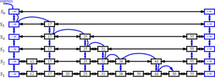
An example of a skip list is shown in Figure 1. It is customary to visualize a skip list S with sequence S

at the bottom and sequences S

::: S

above it. Also, we refer to h as the height of skip list S .

17 31 38

55 50

12 17 20 25 31 38 39 44

44 12

17 31 55

17

17 55

55 25

25 25 S6

S5 S₄ S3 S2 S1 find(50)

8

-

8

-

8

-

8

-

8

-

8

- +8

8+

8

+

8

+

8+

8

+

Figure 1: Example of a skip list. The dashed lines show the traversal of the structure performed when searching for key 50.

Intuitively, the sequences are set up so that S

con- tains more or less every other item in S

. As we shall see in the details of the insertion method, the items in S

are chosen at random from the items in S

by picking each item from S

to also be in S

with probability 1 = 2. That is, in essence, we \ip a coin" for each item in S

and place that item in S

if the coin comes up

\heads." Thus, we expect S

to have about n= 2 items, S

to have about n= 4 items, and, in general, S

to have about n= 2

items. In other words, we expect the height h of S to be about log n .

Using the position abstraction used previously by the authors 2] for nodes in sequences and trees, we view a skip list as a two-dimensional collection of positions ar- ranged horizontally into levels and vertically into tow- ers. Each level corresponds to a sequence S

and each tower contains positions storing the same item across consecutive sequences. The positions in a skip list can be traversed using the following operations:

after ( p ): the position following p on the same level.

before ( p ): the position preceding p on the same level.

below ( p ): the position below p in the same tower.

above ( p ): the position above p in the same tower.

Without going into the details, we note that we can eas- ily implement a skip list by means of a linked structure such that the above traversal methods each take O (1) time, given a skip-list position p .

2.2 Searching

The skip list structure allows for simple dictionary search algorithms. In fact, all of the skip list search algorithms are based on an elegant SkipSearch method that takes a key k and nds the item in a skip list S with the largest key (which is possibly

) that is less than or equal to k . Suppose we are given such a key k . We begin the SkipSearch method by setting a position variable p to the top-most, left position in the skip list S . That is, p is set to the position of the special item with key

in S

. We give a pseudo-code description of the skip-list search algorithm in Code Fragment 1 (see also Figure 1).

Algorithm ^{SkipSearch ( k ):}

Input:

A search key k

Output:

Position p in S such that the item at p has the largest key less than or equal to k

Let p be the topmost-left position of S (which should have at least 2 levels).

while ^below ( p )

= null do

p

below ( p )

drop down

while ^{key ( after ( p ))}

^k do

Let p

after ( p )

scan forward

end while end while return ^{p .}

Code Fragment 1: A generic search in a skip list

.

2.3 Update Operations

Another feature of the skip list data structure is that, be- sides having an elegant search algorithm, it also provides simple algorithms for dictionary updates.

Insertion

The insertion algorithm for skip lists uses randomization to decide how many references to the new item ( k e ) should be added to the skip list. We begin the inser- tion of a new item ( k e ) into a skip list by performing a SkipSearch ( k ) operation. This gives us the position p of the bottom-level item with the largest key less than or equal to k (note that p may be the position of the special item with key

). We then insert ( k e ) in this bottom-level list immediately after position p . After in- serting the new item at this level we \ip" a coin. That is, we call a method random () that returns a number be- tween 0 and 1, and if that number is less than 1 = 2, then we consider the ip to have come up \heads" otherwise, we consider the ip to have come up \tails." If the ip comes up tails, then we stop here. If the ip comes up heads, on the other hand, then we backtrack to the pre- vious (next higher) level and insert ( k e ) in this level at the appropriate position. We again ip a coin if it comes up heads, we go to the next higher level and re- peat. Thus, we continue to insert the new item ( k e ) in lists until we nally get a ip that comes up tails. We link together all the references to the new item ( k e ) created in this process to create the tower for ( k e ). We give the pseudo-code for this insertion algorithm for a skip list S in Code Fragment 2. Our insertion algorithm uses an operation insertAfterAbove ( p q ( k e )) that inserts a position storing the item ( k e ) after position p (on the same level as p ) and above position q , returning the po- sition r of the new item (and setting internal references so that after , before , above , and below methods will work correctly for p , q , and r ).

Algorithm SkipInsert ( k e ):

p

SkipSearch ( k )

q

insertAfterAbove ( p null ( k e ))

while random () < 1 = 2 do while ^{above ( p ) = null} do

p

before ( p )

scan backward

end while

p

above ( p )

jump up to higher level

q

insertAfterAbove ( p q ( k e ))

end while

Code Fragment 2: Insertion in a skip list, assuming random () returns a random number between 0 and 1, and we never insert past the top level.

Removal

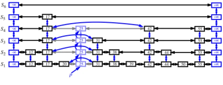
Like the search and insertion algorithms, the removal algorithm for a skip list S is quite simple. In fact, it is even easier than the insertion algorithm. Namely, to perform a remove ( k ) operation, we begin by performing a search for the given key k . If a position p with key k is not found, then we indicate an error condition. Other- wise, if a position p with key k is found (on the bottom level), then we remove all the positions above p , which are easily accessed by using above operations to climb up the tower of this item in S starting at position p (see Figure 2).

38

55 50

12 17 38 39 44

44 12

17 55

17

55

55 S6

S₅ S₄ S₃ S2

S1 42

42 42 42

p 31 31 31 25 25 25 25 20 17

8

-

8

-

8

-

8

-

8

-

8

-

17

8+ 8+ 8+ 8+ 8+ 8+

Figure 2: Removal of the item with key 25 from a skip list.

The positions visited are in the tower for key 25.

2.4 A Simple Analysis of Skip Lists

Our probabilistic analysis of skip lists, which is a sim- plied version of an analysis of Motwani and Ragha- van 4], requires only elementary probability concepts, and it does not need any assumptions about input dis- tributions. We begin this analysis by studying the height h of S .

The probability that a given item is stored in a po- sition at level i is equal to the probability of getting i consecutive heads when ipping a coin, that is, this prob- ability is 1 = 2

. Thus, the probability P

that level i has at least one item is at most

P

n 2

for the probability that any one of n dierent events occurs is at most the sum of the probabilities that each occurs.

The probability that the height h of S is larger than i is equal to the probability that level i has at least one item, that is, it is no more than P

. This means that h is larger than, say, 3log n with probability at most

P

n

2

= n n

^{= 1} n

:

More generally, given a constant c > 1, h is larger than c log n with probability at most 1 =n

. Thus, with high probability, the height h of S is O (log n ).

Consider the running time of a search in skip list S ,

and recall that such a search involves two nested while

loops. The inner loop performs a scan forward on a level of S as long as the next key is no greater than the search key k , and the outer loop drops down to the next level and repeats the scan forward iteration. Since the height h of S is O (log n ) with high probability, the number of drop-down steps is O (log n ) with high probability.

So we have yet to bound the number of scan-forward steps we make. Let n

be the number of keys examined while scanning forward at level i . Observe that, after the key at the starting position, each additional key ex- amined in a scan-forward at level i cannot also belong to level i + 1. If any of these items were on the previous level, we would have encountered them in the previous scan-forward step. Thus, the probability that any key is counted in n

is 1 = 2. Therefore, the expected value of n

is exactly equal to the expected number of times we must ip a fair coin before it comes up heads. This expected value is 2. Hence, the expected amount of time spent scanning forward at any level i is O (1). Since S has O (log n ) levels with high probability, a search in S takes the expected time O (log n ). By a similar analy- sis, we can show that the expected running time of an insertion or a removal is O (log n ).

Finally, let us turn to the space requirement of a skip list S . As we observed above, the expected number of items at level i is n= 2

, which means that the expected total number of items in S is

h

X

i=0

2 n

= n

i=0

2 1

< 2 n:

Hence, the expected space requirement of S is O ( n ).

3 Sorting

One of the most popular sorting algorithms is the quick- sort algorithm, which uses a pivot element to split a sequence and then it recursively sorts the subsequences.

One common method for analyzing quick-sort is to as- sume that the pivot will always divide the sequence al- most equally. We feel such an assumption would pre- suppose knowledge about the input distribution that is typically not available, however. Since the intuitive goal of the partition step of the quick-sort method is to divide the sequence S almost equally, let us introduce random- ization into the algorithm and pick as the pivot a random element of the input sequence. This variation of quick- sort is called randomized quick-sort, and is provided in Code Fragment 3.

There are several analyses showing that the expected running time of randomized quicksort is O ( n log n ) (e.g., see 1, 4, 8]), independent of any input distribution as- sumptions. The analysis we give here simplies these analyses considerably.

Our analysis uses a simple fact from elementary prob- ability theory: namely, that the expected number of

Algorithm ^quickSort ( S ):

Input:

Sequence S of n comparable elements

Output:

A sorted copy of S

if ^{n = 1} then return ^{S .} end if

pick a random integer r in the range 0 n

1]

let x be the element of S at rank r . put the elements of S into three sequences:

L , storing the elements in S less than x E , storing the elements in S equal to x G , storing the elements in S greater than x . let L

quickSort ( L )

let G

quickSort ( G )

return ^L

+ E + G

.

Code Fragment 3: Randomized quick-sort algorithm.

times that a fair coin must be ipped until it shows

\heads" k times is 2 k . Consider now a single recursive invocation of randomized quick-sort, and let m denote the size of the input sequence for this invocation. Say that this invocation is \good" if the pivot chosen is such that subsequences L and G have size at least m= 4 and at most 3 m= 4 each. Thus, since the pivot is chosen uni- formly at random and there are m= 2 pivots for which this invocation is good, the probability that an invocation is good is 1 = 2.

Consider now the recursion tree T associated with an instance of the quick-sort algorithm. If a node v of T of size m is associated with a \good" recursive call, then the input sizes of the children of v are each at most 3 m= 4 (which is the same as m= (4 = 3)). If we take any path in T from the root to an external node, then the length of this path is at most the number of invocations that have to be made (at each node on this path) until achiev- ing log

n good invocations. Applying the probabilistic fact reviewed above, the expected number of invocations we must make until this occurs is at most 2log

n . Thus, the expected length of any path from the root to an external node in T is O (log n ). Observing that the time spent at each level of T is O ( n ), the expected run- ning time of randomized quick-sort is O ( n log n ).

4 Selection

The selection problem we asks that we return the k th

smallest element in an unordered sequence S . Again

using randomization, we can design a simple algorithm

for this problem. We describe in Code Fragment 4 a

simple and practical method, called randomized quick-

select, for solving this problem.

Algorithm quickSelect ( S k ):

Input:

Sequence S of n comparable elements, and an integer k

1 n ]

Output:

The k th smallest element of S

if ^{n = 1} then

return the (rst) element of S .

end if

pick a random integer r in the range 0 n

1]

let x be the element of S at rank r . put the elements of S into three sequences:

L , storing the elements in S less than x E , storing the elements in S equal to x G , storing the elements in S greater than x .

if ^k

^L

then

quickSelect( L k )

else if ^k

^L

⁺

^E

then

return ^x

each element in E is equal to x

else quickSelect( G k

L

E

)

end if

Code Fragment 4: Randomized quick-select algorithm.

We note that randomized quick-select runs in O ( n

) worst-case time. Nevertheless, it runs in O ( n ) expected time, and is much simpler than the well-known deter- ministic selection algorithm that runs in O ( n ) worst-case time (e.g., see 1]). As was the case with our quick-sort analysis, our analysis of randomized quick-select is sim- pler than existing analyses, such as that in 1].

Let t ( n ) denote the running time of randomized quick-select on a sequence of size n . Since the random- ized quick-select algorithm depends on the outcome of random events, its running time, t ( n ), is a random vari- able. We are interested in bounding E ( t ( n )), the ex- pected value of t ( n ). Say that a recursive invocation of randomized quick-select is \good" if it partitions S , so that the size of L and G is at most 3 n= 4. Clearly, a re- cursive call is good with probability 1 = 2. Let g ( n ) denote the number of consecutive recursive invocations (includ- ing the present one) before getting a good invocation.

Then t ( n )

bn

g ( n ) + t (3 n= 4)

where b

1 is a constant (to account for the overhead of each call). We are, of course, focusing in on the case where n is larger than 1, for we can easily characterize in a closed form that t (1) = b . Applying the linearity of expectation property to the general case, then, we get

E

(

(

))

(

(

) +

(3

4)) =

(

(

))+

(

(3

4))

Since a recursive call is good with probability 1 = 2, and whether a recursive call is good or not is independent

of its parent call being good, the expected value of g ( n ) is the same as the expected number of times we must ip a fair coin before it comes up \heads." This implies that E ( g ( n )) = 2. Thus, if we let T ( n ) be a shorthand notation for E ( t ( n )) (the expected running time of the randomized quick-select algorithm), then we can write the case for n > 1 as T ( n )

T (3 n= 4)+2 bn . Converting this recurrence relation to a closed form, we get that

T ( n )

2 bn

dlog

4=3 ne

X

i=0

(3 = 4)

:

Thus, the expected running time of quick-select is O ( n ).

5 Conclusion

We have discussed the use of randomization in teaching several key concepts on data structures and algorithms.

In particular, we have presented simplied analyses for skip lists and randomized quick-sort, suitable for a CS2 course, and for randomized quick-select suitable for a DS&A course.

These simplied analyses, as well as some additional ones, can also be found in the recent book on data struc- tures and algorithms by the authors 2]. The reader interested in further study of randomization in data structures and algorithms is also encouraged to examine the excellent book on Randomized Algorithms by Mot- wani and Raghavan 4] or the interesting book chapter by Seidel on \backwards analysis" of randomized algo- rithms 8].

References

1] T. H. Cormen, C. E. Leiserson, and R. L. Rivest. In- troduction to Algorithms . MIT Press, Cambridge, MA, 1990.

2] M. T. Goodrich and R. Tamassia. Data Structures and Algorithms in Java . John Wiley and Sons, New York, 1998.

3] P. Kirschenhofer and H. Prodinger. The path length of random skip lists. Acta Informatica , 31:775{792, 1994.

4] R. Motwani and P. Raghavan. Randomized Algorithms . Cambridge University Press, New York, NY, 1995.

5] T. Papadakis, J. I. Munro, and P. V. Poblete. Average search and update costs in skip lists. BIT , 32:316{332, 1992.

6] P. V. Poblete, J. I. Munro, and T. Papadakis. The bi- nomial transform and its application to the analysis of skip lists. In Proceedings of the European Symposium on Algorithms (ESA) , pages 554{569, 1995.

7] W. Pugh. Skip lists: a probabilistic alternative to bal- anced trees. Commun. ACM , 33(6):668{676, 1990.

8] R. Seidel. Backwards analysis of randomized geometric

algorithms. In J. Pach, editor, New Trends in Discrete

and Computational Geometry , volume 10 of Algorithms

and Combinatorics , pages 37{68. Springer-Verlag, 1993.