Compositional differences of fluorescent dissolved organic matter in Arctic Ocean spring sea ice and surface waters north of Svalbard

(1)

Contents lists available at ScienceDirect

Marine Chemistry

journal homepage: www.elsevier.com/locate/marchem

Compositional differences of fluorescent dissolved organic matter in Arctic Ocean spring sea ice and surface waters north of Svalbard

Monika Zabłocka

^a,^⁎

, Piotr Kowalczuk

^a

, Justyna Meler

^a

, Ilka Peeken

^b

, Katarzyna Dragańska-Deja

^a

, Aleksandra Winogradow

^a

a Institute of Oceanology Polish Academy of Sciences, ul. PowstańcówWarszawy 55, PL-81-712 Sopot, Poland

b Alfred-Wegener-Institut Helmholtz-Zentrum für Polar- und Meeresforschung, Polar Biological Oceanography, Bremerhaven, Germany

A R T I C L E I N F O Keywords:

Arctic Ocean

Sea ice optical properties

Fluorescent dissolved organic matter (FDOM) PARAFAC - parallel factor analysis

A B S T R A C T

We assessed the qualitative composition of fluorescent dissolved organic matter (FDOM) in Arctic Ocean surface water and in sea ice north of the Svalbard Archipelago (in the Sophia Basin, the Yermak Plateau and the north Spitsbergen shelf) in May and June 2015, during the “TRANSSIZ” expedition (Transitions in the Arctic Seasonal Sea Ice Zone). Samples collected in open lead waters (OW), under-ice waters (UIW) and from the sea ice (ICE) were analyzed by fluorescence spectroscopy and subsequently by multivariate statistical methods using Parallel Factor Analysis (PARAFAC). Statistical analyses of all measured DOM fluorescence excitation and emission matrices (EEMs) enabled four components to be identified and validated. The spectral characteristics of the first component C1 (λEx/λEm 282(270)/335) corresponded to those of tryptophan. The spectral properties of the other three components corresponded to those of humic-like substances: components two (C2 − λEx/λEm

315(252)/395) and three (C3 − λEx/λEm 357(258)/446) corresponded to humic-like substances of marine origin, whereas component four (C4 − λEx/λEm 261(399)/492) resembled terrestrial humic-like substances.

Changes in FDOM composition were recorded in OW, in contrast to UIW and sea ice. In the OW the sum of fluorescence intensities of humic-like components (C2, C3 and C4) was two times higher than the fluorescence intensity of protein-like component (C1). Component C2 exhibited the highest fluorescence intensity. In the UIW and particularly in the sea ice the fluorescence intensity of the protein-like component, IC1, was the highest. The IC1 in the sea ice increased toward the sea ice bottom, reaching maximum values at the sea ice-water interface.

The calculated spectral indices (SUVA(254) and HIX) and ratios of fluorescence intensities of protein-like to humic-like components, Ip/Ih, suggested that FDOM in water and sea ice was predominantly autochthonous, characterized by low molecular weight organic compounds and low aromatic ring saturation. Enrichment factors Dc, calculated from salinity-normalized values of the optical DOM properties and dissolved organic carbon concentrations, indicated the significant fractionation of FDOM in the sea ice relative to the parent open waters.

The humic-like terrestrial component C4 was enriched the least, whereas the protein-like component C1 was enriched the most. A statistically significant (p < 0.0001) and relatively strong (R = 63) correlation between IC1

and the total chlorophyll a concentration Tchla was found in the sea ice, which suggests that sympagic algal communities were producers of the protein-like FDOM fraction.

1. Introduction

Sea ice differs significantly from other constituents of Earth's cryosphere that originate from freshwater or snow (lake ice, glaciers). The difference is due to sea salt ions, which impact on the formation of ice, its crystalline structure, and its physical and chemical properties (Thomas, 2017 and re- ferences therein). Sea ice forms a boundary layer in polar and subpolar marine basins. This insulating layer reduces the heat, mass and momentum exchange between the ocean and atmosphere (McPhee, 2017), alters the

surface albedo and reduces radiative energy transfer to the underlying water, which affects the heating rate and primary production by sympagic algae communities and under-ice phytoplankton (Arrigo, 2017). Sea ice, especially in the Arctic Ocean and Antarctica, is a key factor regulating global climatic processes through the so-called sea ice albedo feedback. The sea ice albedo changes seasonally and spatially, and is strongly dependent on sea ice surface properties, reaching a maximum of 0.85 in early spring for snow-covered ice and a minimum in late summer (0.2) for melt pond- covered ice (Perovich, 2017; Perovich et al., 1993; Taskjelle et al., 2016).

https://doi.org/10.1016/j.marchem.2020.103893

Received 24 March 2020; Received in revised form 7 September 2020; Accepted 16 September 2020

⁎Corresponding author.

E-mail address: monika_z@iopan.pl (M. Zabłocka).

Available online 07 October 2020

T

(2)

With increasing fragmentation of the sea ice cover and the appearance of cracks and leads, the sea ice albedo falls to < 0.2. The rate of solar energy being transmitted through the sea ice depends not only on its thickness, surface properties and fragmentation, but also on the inherent optical properties of the sea ice, i.e., its scattering and absorption coefficients (Perovich, 2017; Taskjelle et al., 2017; Katlein et al., 2019).

The spectral properties and magnitudes of the absorption and scattering coefficients of bulk sea ice depend not only on its crystal structure, the presence of brine channels and impurities such as gas bubbles and particles, but also on the concentration, composition and vertical distribution of absorbing and scattering constituents (Grenfell and Perovich, 1981; Perovich and Govoni, 1991). The absorption and scattering coefficients vary seasonally in magnitude as a result of temporal changes in concentrations of optically significant sea ice constituents contributing to the bulk inherent optical properties and their spectral transformations (Light et al., 2015;

Katlein et al., 2019). Assuming that gas bubbles and inorganic sea salt ions do not significantly absorb light at wavelengths greater than 350 nm (Woźniak and Dera, 2007), the main contributors to the sea ice absorption, as in oceanic waters, are ice crystals (water), dissolved and particulate organic matter, particulate mineral matter contained in the ice and brine, and algae growing in the sea ice itself.

Chromophoric dissolved organic matter (CDOM – the optically active fraction of dissolved organic matter DOM) is one of the most optically significant sea water constituents, strongly absorbing light in the UV and visible wavelength ranges. Its absorption spectrum decreases exponentially with increasing wavelengths (Jerlov, 1976). Part of CDOM, known as fluorescent dissolved organic matter (FDOM), has the inherent ability to emit a fraction of the absorbed energy as fluorescence. This property has been known since the late 1930s (Kalle, 1938) and has been used to esti- mate CDOM in a range of natural waters (Vodacek et al., 1997; Ferrari and Dowell, 1998; Ferrari, 2000). With Excitation Emission Matrix (EEM), a fluorescence spectroscopy technique utilizing emission spectra measurements at a series of successively increasing excitation wavelengths, local fluorescence intensity maxima occurring within characteristic excitation and emission ranges can be assigned to broad classes of dissolved organic compounds constituting DOM (Coble, 1996). Parallel Factor Analysis is a multivariate statistical method which application to DOM biogeochemistry has enabled objective interpretation of EEM spectra and discrimination of different classes of fluorophores based on their excitation/emission maxima (Stedmon et al., 2003). This approach has been used to interpret the mul- tidimensional nature of EEM data sets, and also to study FDOM variability in coastal areas (Stedmon and Markager, 2005a; Kowalczuk et al., 2009), open oceans (Jørgensen et al., 2011; Kowalczuk et al., 2013; Catalá et al., 2016) and in the Arctic Ocean (Dainard and Guéguen, 2013; Guéguen et al., 2014, 2015; Gonçalves-Araujo et al., 2015, 2016). It has improved our understanding of DOM production and degradation in the marine en- vironment (Stedmon and Markager, 2005b), as well as enabling water masses of different origin to be tracked (Gonçalves-Araujo et al., 2016).

The properties of CDOM and FDOM in the sea ice have been studied during different phases of its formation, persistence and melting, mostly in the Baltic Sea, (Ehn et al., 2004; Stedmon et al., 2007; Uusikivi et al., 2010; Müller et al., 2011), the Chukchi Sea and Canadian Arctic (Xie et al., 2014; Logvinova et al., 2016; Hill and Zimmerman, 2016), Ant- arctica (Norman et al., 2011), and in indoor experiments under con- trolled conditions (Müller et al., 2011, 2013). It has been found that a high proportion of DOM/CDOM is rejected from the ice crystal structure with the brine during ice formation, although a small fraction of it remains incorporated within the ice and persists in brine channels (Müller et al., 2013; Hill and Zimmerman, 2016). During the ice formation, DOM remaining in the ice undergoes significant fractionation.

The humic-like fraction is the most susceptible to rejection from the sea ice along with the brine during freezing, whereas the protein-like DOM fraction is the least susceptible to this process, which shifts the molecular composition of DOM toward a higher proportion of low molecular weight (LMW) compounds (Müller et al., 2013; Granskog et al., 2015b;

Retelletti-Brogi et al., 2018). The intensive growth of sympagic algae in

spring and the associated production of organic matter further con- tribute to the accumulation of LMW organic matter in the sea ice (Stedmon et al., 2007). Significant in situ production of DOM/CDOM by sympagic autotrophic organisms inhabiting land-fast sea ice in the Canadian Archipelago was documented by Xie et al. (2014). The composition of DOM/CDOM and its associated optical properties may be further modified by photochemical and microbial transformations (Stedmon et al., 2007).

The optical properties of the sea ice north of Svalbard were described by Kowalczuk et al. (2017) and Kauko et al. (2017), who reported much lower CDOM absorption in the sea ice and under-ice waters than in the Western Arctic Ocean and over the Siberian Shelf. The properties, distribution and cycling of FDOM in the sea ice in the Atlantic sector of the Arctic Ocean have not been studied to date. The main aim of this research was to: i) assess the DOM composition in the sea ice and underlying waters in early spring on the basis of fluorescence spectroscopy, multivariate statistical models (PARAFAC) and calculated spectral indices; ii) analyze the distribution of identified FDOM components and spectral indices in the vertical profiles within the sea ice and under-ice water; iii) relate measured DOM optical signatures to concentrations of dissolved organic carbon and chlorophyll a.

2. Materials and methods 2.1. The study area

Sea ice and water samples were collected north of Svalbard, in the northern extension of its shelf, the Sophia Basin and the Yermak Plateau (Table 1, Fig. 1). This is an important region, where warm Atlantic Water (AW) carrying heat and salt into the Arctic Ocean interfaces Polar Water (PW) (Aagaard et al., 1987). More than 30% of the total AW that flows through the Fram Strait into the Arctic is carried by the West Spitsbergen Current (WSC) (Beszczynska-Möller et al., 2012), a northward flowing extension of the Norwegian Atlantic Current (NAC).

At about 80°N, WSC splits into two branches: the Svalbard Branch (SB) and the Yermak Plateau Branch (YPB). The SB follows the continental shelf while the YPB moves northwestward until about 81°N, where warm WSC waters meet ice transported by the Transpolar Drift from the eastern Arctic seas north of Svalbard. This region, known as Whalers Bay, has become ice-free as a result of intense ice melting (Onarheim et al., 2014). Apart from melting the ice from below (Polyakov et al., 2017), the Atlantic waters also inhibit ice growth during winter. In consequence, during the last few decades, the ice edge as a whole has been retreating farther north of Svalbard. The largest contraction of the ice north of Svalbard occurs during winter, which is in contrast to the changes observed in central parts of the Arctic Ocean (Onarheim et al., 2014). Increasing volumes of warm AW intrusions have caused the ice pack carried by the Transpolar Drift to move into thinner and younger sea ice during recent decades (Hansen et al., 2013; Renner et al., 2014).

2.2. Sample collection and processing

Water and sea ice samples were collected during the “TRANSSIZ”

expedition (Transitions in the Arctic Seasonal Sea Ice Zone) on board the icebreaker FS Polarstern in May and June 2015 (cruise code PS92 - ARK XXIX/1) (Peeken, 2016). The field work was conducted in the sea ice covered waters. All together we collected 84 OW samples, 16 UIW samples and 58 ICE samples. Detailed information on the water and sea ice-water stations visited during the cruise is given in Table 1.

2.2.1. Sea ice sampling

Sea ice sampling involved the collection of sea ice for determining biological, physical and chemical parameters with Kovacs Mark II or Mark V coring systems (Kovacs Enterprise, Roseburg, USA). Three separate sea ice cores were collected in order to obtain the parameters discussed in this article: one physical core, which was used to measure temperature and salinity, CDOM absorption and dissolved organic carbon concentration; and

(3)

another two for determining biological variables, including the chlorophyll a concentration (from pigment analysis). The temperature in the physical core was measured with a Testo 720 probe (Testo Electronics, Lenzkirch, Germany) every 5 cm. Thereafter, the core was cut into 10 cm sections, placed in acid-cleaned high-density polyethylene (HDPE) cups and immediately stored in a cooling box prior to transportation to the ship. Because of the high concentration of algae at the bottom of the ice core, the length of the last (bottom) section was 5 cm. One of the “biological” cores was also

cut into 10 cm pieces, except for the last 5 cm, which was pooled with the last 5 cm section from the second “biological” core (to obtain a sufficient volume of melt water). All the “biological” core sections were melted in sea water previously passed through a 0.2 μm filter in order to minimize the osmotic stress on protists during the melting process (Miller et al., 2015).

Sections from the cores were stored in a fridge at 4 °C and kept in the dark until melted. In the physical core, salinity was measured with a Salinometer WTW Cond 3110 (Wissenschaftlich-Technische Werkstätten, Weilheim, Germany) and the remaining water was used for all the variables except chlorophyll a. To obtain the volume of the melt water required for mea- suring the biological parameters listed above, water from two adjacent sections, starting from the sea ice surface, was pooled. The last 5 cm sections were not pooled with the overlying ice sections.

2.2.2. Water sampling

Water column samples from the open lead waters (OW) were collected with a rosette water sampler system (Sea-Bird Electronics Inc.), deployed by the side of the ship and equipped with 24 12-l Niskin bottles. The water column was sampled at the depths – 5, 10, 20, 30, 75, 100 m and just above the sea bed. Additionally, at every ice station, the under-ice water (UIW) was collected using a Kemmerer-type bottle deployed manually through the drill holes from which the sea ice cores were extracted. UIW was sampled directly from beneath the sea ice cover (0 m) and from the chlorophyll a maximum depth, determined with a CYCLOPS-7 submersible fluorometer (Turner Designs, Sunnyvale, CA, USA), attached to a Sea and Sun CTD75M probe (Sea and Sun Technology, Trappenkamp, Germany). The CTD75M probe was lowered manually through an sea ice hole. The depth of the Kemmerer bottle sampling was measured with a metered rope.

2.2.3. Sample processing

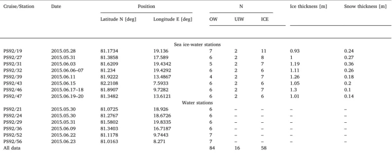
Water column samples collected for CDOM, FDOM and DOC concentration were filtered gravitationally through an Opticap XL4 Durapore flow-through filter cartridge of nominal pore size 0.2 μm, attached directly to the Niskin bottle tap. To prevent sample con- tamination, the cartridge filter and tubing were stored in 10% aq. HCl and rinsed with ultrapure MilliQ and sample water before sample collection. Sea ice melt water (ICE) samples and UIW samples for determining CDOM, FDOM and DOC were filtered twice: once through Whatman glass-fiber filters (GF/F, nominal pore size 0.7 μm) and then through acid-washed Sartorius 0.2 μm pore size cellulose membrane Table 1

Dates, positions, number of samples (N) collected in OW, UIW and ICE and parameters measured during the TRANSSIZ expedition.

Cruise/Station Date Position N Ice thickness [m] Snow thickness [m]

Latitude N [deg] Longitude E [deg] OW UIW ICE

Sea ice-water stations

PS92/19 2015.05.28 81.1734 19.136 7 2 11 0.93 0.24

PS92/27 2015.05.31 81.3858 17.589 6 2 8 1 0.27

PS92/31 2015.06.03 81.6209 19.4342 5 2 7 1.19 0.36

PS92/32 2015.06.06–07 81.234 19.4292 6 2 6 1.11 0.26

PS92/39 2015.06.11 81.9222 13.4867 4 2 7 1.26 0.18

PS92/43 2015.06.15 82.2108 7.5933 6 2 6 1.05 0.2

PS92/46 2015.06.17–18 81.8907 9.7282 6 2 7 1.3 0.1

PS92/47 2015.06.19–20 81.3482 13.6121 6 2 6 1.01 0.14

Water stations

PS92/21 2015.05.30 81.0725 18.926 6 – – – –

PS92/24 2015.05.30 81.2767 18.6726 6 – – – –

PS92/29 2015.05.31 81.5802 19.8335 6 – – – –

PS92/36 2015.06.09 81.3403 16.7187 6 – – – –

PS92/52 2015.06.22 81.1178 9.7443 7 – – – –

PS92/56 2015.06.23 81.0163 8.271 7 – – – –

All data 84 16 58

Note: Sampling of the physical, optical and bio-optical parameters during the TRANSSIZ cruise included temperature, salinity, aCDOM(λ), FDOM, chlorophyll a concentration, Tchla, and was conducted in: the open leads water column (OW), under sea ice water column (UIW) and sea ice (ICE).

Fig. 1. Location of the sampling stations during the TRANSSIZ (PS92) expedi- tion.

(4)

filters. The 0.2 μm sterile syringe filter (VWR cellulose acetate membrane) attached to a 150 mL acid-washed plastic syringe were used to filter sea ice melt water from the last 5 cm sea ice cores sections to collect CDOM, FDOM and DOC samples. The samples for determining DOC were acidified with 150 μL 0.1 M HCl. All samples were filtered into pre-combusted amber glass vials and stored at 4 °C in the dark, which preserves DOM optical properties for several weeks (Stedmon and Markager, 2001).

Water column, UIW and melted sea ice samples collected for HPLC (high performance liquid chromatography) pigment analysis were passed through Whatman 25 mm GF/F filters. The filter pads with material retained on them were immediately immersed in liquid ni- trogen and thereafter stored at −80 °C prior to analysis.

2.2.4. CDOM absorption measurements

During the TRANSSIZ expedition, CDOM absorption was measured on board the FS Polarstern immediately after filtration using a double- beam Perkin-Elmer Lambda-35 spectrophotometer in the spectral range 240–700 nm. The measurements were done in a 10-cm quartz cell, with fresh ultrapure water as reference. The CDOM absorption coefficient aCDOM(λ) was calculated using the equation:

=

aCDOM( ) 2.303 ( )/A l (1)

where A(λ) is the absorbance, l is the optical path length in meters and the factor 2.303 is the natural logarithm of 10.

The CDOM absorption spectrum slope coefficient S350-600 was calculated in the 350–600 nm spectral range using a nonlinear least squares fitting method with the Trust-Region algorithm implemented in Matlab R2013 (Stedmon et al., 2000; Kowalczuk et al., 2006). The method uses the equation:

= +

a_CDOM( ) a_CDOM( )₀ e ^S⁽⁰ ⁾ K (2) where λ0 is 350 nm, and K is a background constant of the baseline shift resulting from the residual scattering by fine size particle fractions, micro-air bubbles or colloidal material present in the sample, refractive index differences between the sample and the reference, or attenuation not due to CDOM.

2.2.5. DOM fluorescence measurements and the PARAFAC model Fluorescence Excitation Emission Matrix spectra (EEM) of the DOM samples collected during TRANSSIZ were measured in the laboratory at the Institute of Oceanology Polish Academy of Sciences (IOPAN – Sopot, Poland) with a HORIBA Aqualog spectrofluorometer in a 1 cm quartz cuvette. The excitation spectral range was set at 240–600 nm with a 3 nm increment. The emission spectral range was recorded between 246.65 and 829.44 nm with a 2.33 nm increment. The emission signal integration time was 8 s. All the EEM spectra acquired were spectrally corrected with a set of instrument-dependent correction coefficients internally implemented within the spectrofluorometer.

The excitation and emission matrix spectra were processed using the drEEM toolbox implemented in the Matlab 2013R computing environ- ment, in accordance with the procedures described by Stedmon and Bro (2008) and Murphy et al. (2010, 2013). The spectrally corrected samples were calibrated and normalized against the Raman scatter emission peak of the MilliQ water sample, run on the same day, excited at a wavelength of 351 nm and integrated in the spectral range 378–424 nm. The resulting EEM spectra were scaled in Raman units (R.U., [nm⁻¹]). Samples were corrected for inner filter effects using the CDOM absorption spectra of the corresponding water samples (section 2.2.4). The blank MilliQ water sample, corrected and calibrated in the same way as the regular samples, was subtracted from each measured EEM to remove the Raman scattering signal. The PARAFC model was applied to the data array, the dimensions of which consisted of 168 samples × 121 excitations × 153 emissions. The PARAFAC model was run with a non-negativity constraint on the assumption that signals from a complex mixture of DOM compounds can be separated and that

the components differ from each other spectrally. The PARAFC model results were validated by split-half validation (Harshman, 1984) applied to independent sub datasets (S4C6T3 – Splits, Combinations, Tests). A four component model was successfully validated.

2.2.6. HPLC measurements

The HPLC chlorophyll samples from TRANSSIZ ice melt water were measured using a Waters 1525 binary pump equipped with an auto sampler (OPTIMAS™), a Waters photodiode array and fluorescence detectors (2996, 2475, respectively), and EMPOWER software. To each filter sample 50 μL of canthaxanthin (internal standard) and 1.5 mL of acetone were added and then homogenized for 20 s in a Precellys®

tissue homogenizer. After centrifugation, the supernatant liquids were passed through 0.2 μm PTFE filters (Rotilabo). Aliquots of 100 μL were transferred into the auto sampler (4 °C), premixed with 1 M ammonium acetate solution (1:1) and injected into the HPLC-system. Pigments were analyzed by reverse-phase HPLC using a VARIAN Microsorb-MV3 C8 column (4.6 × 100 mm) and HPLC-grade solvents (Merck). Solvent A consisted of 70% methanol and 30% 1 M ammonium acetate, and solvent B consisted of 100% methanol. The gradient was modified after Barlow et al. (1997). Eluting pigments were detected by absorbance (440 nm) and fluorescence (Ex: 410 nm, Em: > 600 nm), and chlorophyll a was identified by comparing their retention times with those of pure standards. Additional confirmation was obtained by comparing the spectra with the on-line diode array absorbance spectra between 390 and 750 nm stored in the library from the pure standards. The total chlorophyll concentration, Tchla, was calculated as the sum of chlorophyll a and its allomers and epimers concentrations measured with HPLC methods.

2.2.7. DOC concentrations

Concentrations of Dissolved Organic Carbon (DOC) were measured in a HiPerTOC analyzer (Thermo Electron Corp., the Netherlands). The method used was based on UV/persulphate oxidation and NDIR (Non Dispersive Infra-Red) detection of evolving CO2 (Sharp, 2002). To remove dissolved CO2, each sample was purged with synthetic air. The precision of the measurement was determined from a triplicate analysis of each sample. Quality control consisted of the regular analysis of blanks as well as accuracy checks based on comparisons with the reference material supplied by the Dennis Hansell Laboratory (University of Miami). The methodology ensured satisfactory accuracy (average recovery 93.1% of the certified CRM value; n = 5) and precision characterized by a relative standard deviation (RSD) of 2.5%.

2.2.8. Spectral indices

Following spectral indices, widely used in aquatic DOM biogeochemistry, based on CDOM absorption and DOM fluorescence spectra were calculated to quantify structural and compositional changes in DOM: i) humification index – HIX, which is related to C/H ratio in DOM molecular structure, was calculated from the original EEMs, according to Zsolnay et al. (1999) as the ratio of the emission spectrum (excited at 255 nm) integral over the spectral range 434–480 nm, 434Iex

480 ( .255), to the emission spectrum integral over the spectral range 300–346 nm (excited at the same wavelengths),

I_ex

300 346 ( .250):

= = HIX H

L I I

ex ex 480 434 ( .255)

345

300 ( .255) (3)

ii) Ip/Ih calculated as the ratio of the fluorescence intensity of identified protein-like components to the sum of fluorescence intensities of identified humic-like components:

= + +

I I I

p h C

C C C

1

2 3 4 (4)

where ICn is the intensity of the respective component from one through

(5)

four (C1 to C4) identified by the PARAFAC model. The spectral characteristics and origins of these components are explained in the Results section and listed in Table 3.

iii) the carbon specific absorption coefficient at 254 nm – SUVA(254). This describes the relative aromaticity of DOM and is lin- early correlated with the percentage aromatic ring saturation of the DOM mixture (Weishaar et al., 2003); low values refer to DOM with a dominant aliphatic structure and low aromatic ring saturation. This index was calculated as follows:

=

SUVA a

(254) _CDOMDOC(254)

(5) where aCDOM(254) is the CDOM absorption coefficient at 254 nm and DOC is the dissolved organic carbon concentration.

2.2.9. Enrichment factors

During sea ice formation, DOM, together with inorganic dissolved constituents of water, is gradually rejected from the crystalline ice structure. These non-linear processes, leading to the enrichment of CDOM and FDOM in the ice relative to salinity, can be quantified using the formula given by Müller et al. (2011):

=

( ) ( )

D

( )

C S i

C S w C S w c

(6) where C denotes the concentration/quantity of given parameter, S denotes the salinity and subscripts i and w refer to ICE and OW, respectively. The median values of enrichment factors D_cwere calculated for three sea ice sections (surface, middle and bottom) and also for the last

5 cm of the sea ice (Table 6).

We calculated the enrichment factors Dc for the following parameters: CDOM absorption coefficient at 350 nm (aCDOM(350)), the fluorescence intensities of each identified fluorophore (I_C1through I_C4), the total fluorescence intensity (Itot) and the dissolved organic carbon concentration (DOC), normalizing the respective values with respect to the relevant salinity (C/S). As we did not know the initial conditions during ice formation, we assumed after Kowalczuk et al. (2017) that salinity and the optical properties of CDOM and FDOM, i.e. aCDOM(350), ICn, and Itot and DOC, were close to those observed in the surface layer of OW (Tables 2, 4 and 5).

2.2.10. Statistical analysis

The statistical Shapiro-Wilk test has been performed in the initial phase of the data analysis to check whenever analyzed parameter conform the normal distribution. Most of considered parameters failed the conformity with normal distribution, therefore the percentiles and median values were chose to reflect observed distribution of parameters values. The Mann-Whitney U test has been applied to check the significance in reported differences in median values.

3. Results

3.1. Spring hydrological conditions and bio-optical properties of Arctic Ocean waters and sea ice north of Svalbard

The hydrological and bio-optical conditions of OW and UIW have been described in detail by Kowalczuk et al. (2017), Kauko et al. (2017) and Pavlov et al. (2017), who found statistically significant differences Table 2

Ranges of variability, median and 1st and 3rd quartiles of the physical properties of ice and oceanic water and the optical properties of CDOM, in different environments. N – number of measurements.

Samples description Temperature [°C] Salinity Tchla [mg m⁻³] aCDOM(350) [m⁻¹] Spectral slope S350-600[nm⁻¹] Open leads water column

Surface layer (0-35 m) −1.83 to −1.19 33.78–34.43 0.24–10.19 0.100–0.231 0.010–0.017

Median −1.71 34.14 1.92 0.149 0.014

Q1;Q3 −1.77; −1.59 34.04; 34.29 0.36; 4.03 0.140; 0.163 0.013; 0.015

N 39 39 20 38 38

Below chlorophyll max. Layer (35-200 m) −1.83– 2.56 34.13–34.97 0.03–3.09 0.090–0.195 0.012–0.018

Median −0.11 34.64 0.47 0.137 0.014

Q1;Q3 −1.02; 2 01 34.38; 34.89 0.16; 1.74 0.132; 0.150 0,014; 0.015

N 35 35 20 35 35

Under sea ice water column

Surface (0 m) −2.00 to −1.05 26.04–34.06 0.48–4.84 0.152–0.233 0.013–0.018

Median −1.51 27.95 1.57 0.184 0.016

Q1;Q3 −1.73; −1.27 27.46; 31.58 0.59; 2.65 0.161; 0.214 0.016; 0.017

N 8 8 8 8 8

Chlorophyll max. depth (3-25 m) −1.84 to −1.63 33.75–34.47 0.29–7.46 0.128–0.227 0.011–0.017

Median −1.73 34.16 1.81 0.184 0.016

Q1;Q3 −1.81; −1.67 34.10; 34.35 0.60; 3.24 0.153; 0.202 0.015; 0.017

N 7 7 8 8 8

sea ice

Surface layer (0-33.3%), N=19 −3.33 to −0.20 0.05–10.6 0.11–0.82 0.047–0.663 0.013–0.031

Median −1.90 5.60 0.36 0.102 0.020

Q1;Q3 −2.58; −1.00 3.47; 7.85 0.28; 0.58 0.076; 0.159 0.020; 0.023

Middle layer (33.3-66.6%), N=17 −3.33 to −0.58 0.25–7.1 0.15–1.91 0.036–0.197 0.012–0.024

Median −1.98 4.65 0.63 0.061 0.018

Q1;Q3 −2.48; −1.36 0.75; 5.15 0.44; 0.81 0.053; 0.119 0.016; 0.021

Bottom layer (66.6-100%), N=21 −2.87 to −0.98 1.65–3.2 0.39–8.90 0.049–0.465 0.011–0.036

Median −1.60 5.10 2.55 0.156 0.020

Q1;Q3 −2.05; −1.30 4.60; 5.80 0.65; 5.03 0.086; 0.252 0.015; 0.024

(6)

in the bio-optical properties of Arctic Ocean waters in open leads and under sea ice. To be consistent with Kowalczuk et al. (2017), we have applied the same criteria, creating a data subsets according to the vertical distribution of optical properties in water and sea ice. We now summarize selected published results so as to provide a wider context for the current study.

The surface water temperature was near freezing point. That remnant of the cold mixed layer formed in winter reached ca 80 m depth and was present at most stations sampled (Kowalczuk et al., 2017) except PS92/27 and PS92/31 and to a lesser extent PS92/19 and PS92/32. These stations, located near the north Svalbard shelf, lay on the path of inflowing Atlantic waters (AW). Advection of warm AW gave rise to significant thermo- and haloclines, and the depth of the winter mixed layer was reduced to ca 20 m.

Salinities at all ice stations were higher than 34 (Meyer et al., 2017), indicating the strong influence of Atlantic waters. Salinity measurements beneath the sea ice revealed a strong gradient in a thin layer below the sea ice. This feature was observed at all the sea ice stations except PS92/43 and PS92/46 and was an indicator of the initial phase of sea ice melting (Kowalczuk et al., 2017). The chlorophyll a concentration measured in the south-eastern part of the sampled area (four ice-water stations: PS92/19, PS92/27, PS92/32, PS92/47 and three water stations: PS92/21, PS92/24, PS92/36) was high, up to 7.4 mg m⁻³, indicating growth of the under-ice phytoplankton bloom (Pavlov et al., 2017). CDOM absorption was low and within the range of values reported for this area (Pavlov et al., 2015;

Gonçalves-Araujo et al., 2018). The ranges of aCDOM(350) were 0.090–0.231 m⁻¹in OW, 0.128–0.233 m⁻¹in UIW and 0.036–0.663 m⁻¹ in the sea ice (Table 2). The ranges of S350-600 were 0.010–0.018 nm⁻¹in OW, 0.011–0.018 nm⁻¹in UIW and 0.011–0.036 nm⁻¹in the sea ice (Table 2). Median values of a_CDOM(350) in UIW were higher than CDOM absorption in OW and sea ice (Table 2).

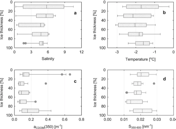
The sea ice varied in thickness from 0.93 to 1.3 m (Table 1). Owing to the considerable variability in the sea ice thickness, the sea ice depth was presented as the percentage core thickness relative to the top of

each core, and all results related to the vertical distribution of the sea ice's physical properties. DOM optical properties were thus expressed as a function of relative thickness. The salinity of sea ice was low – between 0.05 and 10.6 – and its temperature ranged between - 3.33 and - 0.20 °C, which was characteristic of a mixture of first-year and second- year ice (Granskog et al., 2017). The median of sea ice salinity de- creased toward the bottom of the ice, while the lowest median temperature was measured in the middle of sea ice section, with elevated values in the surface and bottom sea ice (Table 2 and Fig. 2).

Median a_CDOM(350) values in the sea ice were similar to those reported in OW but lower than in UIW (Table 2). The vertical distribu- tions of the aCDOM(350) and spectral slope coefficient S350-600 values were elevated at the surface and bottom of the sea ice and minimum median values in the middle of the sea ice, (Fig. 2).

Median Tchla was lower in the sea ice than in OW and UIW (Table 2).

However, chlorophyll a was concentrated in the bottom section of the sea ice (66–100% relative ice depth), with the highest value (8.90 mg m⁻³) in the last 5 cm of the sea ice (on station PS92/31). The Tchla distribution was typically L-shaped (see e.g., Hill and Zimmerman (2016), Kowalczuk et al.

(2017), Kauko et al. (2017)). Tchla increased systematically during the four weeks of observation (Kowalczuk et al., 2017; Kauko et al., 2017; Pavlov et al., 2017), reflecting the increasing light transmission through the sea ice algae biomass (Massicotte et al., 2019).

The DOC levels reported in this study lay within the variability ranges from 33.83 μmol dm⁻³in the middle layer of the sea ice to 139.42 μmol dm⁻³in the OW surface. The range of variability was the smallest in the UIW (70.64–124.83 μmol dm⁻³) and the biggest in the sea ice (139.42–126.17 μmol dm⁻³). Median DOC values were the highest in the UIW reaching 88.25 μmol dm⁻³in water just below the sea ice cover and the smallest in the sea ice (48.25 μmol dm⁻³, in the bottom layer of the ICE). Median DOC values in the OW were between those observed in UIW and ICE (Table 5).

Fig. 2. Vertical profiles of: a) salinity, b) temperature, c) aCDOM(350) and d) S350-600 in the sea ice sections. The sea ice thickness is given as a percentage were 0% is the top of the sea ice and 100% is the bottom of the sea ice (interacting with sea water). Median values are indicated by solid lines, 10th and 90th percentiles by whiskers and 25th and 75th percentiles boxes. The outliers are presented by dots.

(7)

3.2. PARAFAC model output

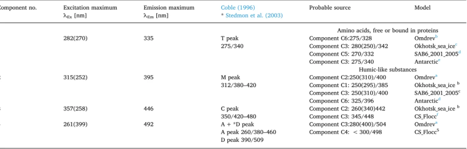
The contour plots and the excitation and emission spectra loadings of the identified components together with the split-half validation results are presented in Fig. 3. The excitation and emission characteristics of the modeled components are listed in Table 3. The PAPRAFAC model identified one protein-like component (C1) and three humic-like components (C2

through C4) in our data set. The excitation/emission characteristics of component one (C1) (λEx/λEm 282(270)/335) resemble the spectral characteristics of tryptophan. Those of component two (C2) (λ_Ex/λ_Em315(252)/

395) resemble the peak M described by Coble (1996), so that C2 is considered to be a precursor of organic matter of marine origin. The second humic-like component C3 (λ_Ex/λ_Em357(258)/446) has spectral characteristics similar to those of the terrestrial humic-like material described by Fig. 3. The PARAFAC output showing the fluorescence signatures of the four components identified in the whole data set. The colorbars indicate the fluorescence intensities in R.U. The line plots ilustrate the spectral shapes of the excitation (dashed lines) and emission (solid lines) of the components.

(8)

Coble (1996) as peak C. We consider the spectral characteristics of the component four (C4) (λEx/λEm 261(399)/492) to be a mixture of humic-like material of terrestrial origin, described earlier as peak A(Coble, 1996), and soil fulvic acids – peak D (Stedmon et al., 2003). We compared the components identified in this study with those identified in different environments by other scientists and stored in the “OpenFluor” spectral library (Murphy et al., 2014). Table 3 compares the spectral properties of FDOM

components identified in this study and matching examples selected from

“OpenFluor” data base.

3.3. Distribution of FDOM components in OW, UIW and sea ice

There were differences in FDOM composition in the two water types (OW and UIW) and the sea ice. The bar plots in Fig. 4 illustrate the median Table 3

Excitation and emission spectral characterization of four components identified by PARAFAC in analyzed data set along with their comparisson with Coble (1996) and other authors (OpenFluor^adatabase).

Component no. Excitation maximum

λEx [nm] Emission maximum

λEm [nm] Coble (1996)

* Stedmon et al. (2003) Probable source Model

Amino acids, free or bound in proteins

1 282(270) 335 T peak

275/340 Component C6:275/328 Omdrev^b

Component C3: 280(250)/342 Okhotsk_sea_ice^c Component C5: 270/332 SAB6_2001_2005^d Component C3: 275/340 Antarctic^e

Humic-like substances

2 315(252) 395 M peak

312/380–420 Component C2:250(310)/400 Omdrev^a

Component C1: 250(295)/385 Okhotsk_sea_ice ^b Component C3: 250(310)/400 SAB6_2001_2005^c Component C6: 325/396 Antarctic^d

3 357(258) 446 C peak

350/420–480 Component C2: 260(340)442 Okhotsk_sea_ice ^b Component C3: 345/448 CS_Flocc^f

4 261(399) 492 A + *D peak

A peak 260/380–460 D peak 390/509

Component C3:280(400)/504 Omdrev^a Component C4: < 300/498 CS_Flocc⁵

a Murphy et al., 2014

b Kothawala et al., 2014

c Granskog et al., 2015b

dKowalczuk et al., 2009

e Stedmon et al., 2011b

f Søndergaard et al., 2003

Fig. 4. Distribution of the fluorescence intesites of compo- nents C1 through C4 in three distinct environments: a) OW – Open Water, b) UIW – Under Ice Water and c) sea ice – ICE.

The sea ice data were additionally split into 4 subsets: surface layer - ICE_SL, middle layer - ICE_ML, bottom layer - ICE_BL, and the last 5 cm in the bottom layer - ICE_last5 (c). The samples from two depth ranges in OW and UIW were pooled together. The bar plots represent the median fluorescence intensities of components C1 through C4.

(9)

fluorescence intensity of each component in the two water masses. The third data set – sea ice (ICE) – was divided into three main vertical subsets:

surface layer, middle layer and bottom layer, with the additional forth layer - last 5 cm layer - subtracted from the bottom layer. The statistical data relating to the total fluorescence intensity I_totand the fluorescence intensities of the PARAFAC components ICn in the two types of water and sea ice and within the specified depth ranges are listed in detail in Table 4. The median I_totwas the lowest in OW (I_tot= 0.042 R.U.) (Table 4). The components in OW in decreasing order of median fluorescence intensity were C2 > C1 > C3 > C4. There was an increase in median Itot (Itot = 0.056 R.U.) and a change in the composition pattern in UIW compared to OW. The components identified in UIW, in decreasing order of median fluorescence intensity ICn, were C1 > C2 > C3 > C4. The median fluorescence intensities of the EEM components ICn were significantly different in OW and UIW, as revealed by the results of the nonparametric Mann-Whitney U test, which measures the significance of differences between median values (Table S1). The FDOM composition, expressed as the mutual proportion of fluorescence intensities of identified components, did not change with depth in either OW or UIW. Median values of the humic-like component C2 were lower by 7.1% in surface OW compared to UIW (Fig. 4).

The decreasing order of median fluorescence intensities of the respective components ICn in the sea ice (all samples) and in the respective vertical sections of the sea ice was much the same as that in UIW (Fig. 4). The only difference between the sea ice sections was in the fluorescence intensity of the components ICn (Fig. 4c). Median Itot was the lowest in the middle of the sea ice (Itot = 0.029 R.U) and the highest at the bottom of the sea ice (Itot = 0.0755 R.U) (Table 4). The fluorescence intensity of the protein-like component C1 was greater than the sum of fluorescence intensities of humic-like components (C2 through C4) in all considered depth section of the sea ice (Fig. 4). The median values of IC1 increased toward the bottom of the sea ice. The I_C1value recorded in the last 5 cm of the sea ice (0.083 R.U) was four times higher than in open waters.

The distribution of the median (as well as averaged) fluorescence intensities of the protein-like component C1 in the sea ice depth profiles was L-shaped, with low IC1 equal to ca 0.010 R.U., uniformly dis- tributed within the upper and middle sections of the sea ice (Fig. 5). IC1

was more than three times greater in the last 20% of the sea ice than in the overlying sea ice layers, and reached its maximum in the last 5 cm of the sea ice (Figs. 4 and 5). The Mann-Whitney U test confirmed the statistical significance of the differences in I_C1values in the sea ice layers. The differences in median IC1 were all found to be statistically significant in the vertical sections of the sea ice except those between the surface and bottom layers (Table S1). The distribution of the median (as well as averaged) fluorescence intensities of the humic-like component C2 in the sea ice depth profiles was higher at the sea ice surface, falling to a local minimum in the middle section of the sea ice, and rising again in the bottom section (Fig. 5). The U test results confirmed that the differences in median IC2 in the middle sea ice section were statistically significant compared to the median IC2 at the surface, in the bottom sections and in the last 5 cm of the sea ice (Table S1). The distribution of the median fluorescence intensities (as well as averaged) of the other two humic-like components IC4 and IC3 in sea ice depth profiles was variable without exhibiting a clear trend (Fig. 5), and the changes in fluorescence intensity of these components were insignif- icant (Table S1). The fluorescence intensities of IC4 in the sea ice were almost one order of magnitude lower than those of IC1, IC2 and IC3

(Fig. 5, Table 4).

3.4. Distribution of spectral indices in the water masses and sea ice 3.4.1. Distribution of SUVA(254) in sampled environments

The changes of DOM composition in the water masses and sea ice were confirmed by the distribution of the median (and also averaged) values of spectral indices (Table 5). The vertical distribution of spectral Table 4

Ranges of variability, median and 1st and 3rd quartiles of fluorescence intensities of four derived components and total fluorescence intensity, in different environments. N – number of measurements.

Samples description IC1 [R.U.] IC2 [R.U.] IC3 [R.U.] IC4 [R.U.] Itot [R.U.]

Open leads water column

Surface layer (0-35 m), N = 39 0.005–0.071 0.008–0.026 0.008–0.20 0.002–0.009 0.025–0.115

Median 0.014 0.014 0.01 0.005 0.044

Q1;Q3 0.011; 0.016 0.013; 0.015 0.009; 0.015 0.005; 0.006 0.041; 0.050

Below chlorophyll max. Layer (35-200 m), N = 35 0.006–0.035 0.009–0.016 0.008–0.019 0.002–0.006 0.031–0.066

Median 0.012 0.014 0.01 0.005 0.042

Q1;Q3 0.010; 0.013 0.013; 0.015 0.010; 0.014 0.005; 0.006 0.039; 0.045

Under sea ice water column

Surface (0 m), N = 14 0.014–0.005 0.015–0.021 0.009–0.018 0.005–0.008 0.046–0.072

Median 0.024 0.015 0.011 0.006 0.056

Q1;Q3 0.019; 0.025 0.015; 0.016 0.010; 0.014 0.006; 0.006 0.055; 0.058

Chlorophyll max. depth (3–25 m), N = 8 0.013–0.060 0.013–0.020 0.010–0.017 0.005–0.008 0.042–0.097

Median 0.024 0.017 0.011 0.006 0.057

Q1;Q3 0.018; 0.032 0.015; 0.019 0.010; 0.013 0.006; 0.007 0.051; 0.072

Sea ice

Surface layer (0 - 33.3 %), N = 19 0.013–0052 0.005–0.019 0.003–0.030 0.001–0.005 0.023–0.105

Median 0.027 0.009 0.007 0.002 0.048

Q1;Q3 0.018; 0.031 0.007; 0.011 0.004; 0.026 0.002; 0.003 0.060; 0.069

Middle layer (33.3 - 66.6 %), N = 17 0.010–0.032 0.004–0.012 0.003–0.029 0.001–0.003 0.018–0.064

Median 0.016 0.007 0.004 0.002 0.03

Q1;Q3 0.014; 0.021 0.005; 0.008 0.004; 0.011 0.001; 0.002 0.026; 0.037

Bottom layer (66.6 - 100 %), N = 21 0.010–0.246 0.006–0.021 0.003–0.031 0.001–0.004 0.020–0.299

Median 0.025 0.009 0.004 0.002 0.055

Q1;Q3 0.016; 0.059 0.007; 0.012 0.003; 0.023 0.001; 0.002 0.028; 0.081

(10)

indices within the sea ice is illustrated in Fig. 6. Low differences in CDOM absorption coefficients between OW, UIW and the sea ice (Table 2), as well as the relatively stable DOC concentration in the water bodies, resulted in a low variability of SUVA(254). Median SUVA(254) was from 3% to 15% higher in UIW than in OW (Table 5).

The distribution of median SUVA(254) within the sea ice was very similar to the distribution of the median Ip/Ih ratio (Fig. 5). Median SUVA(254) in the sea ice was 6% to 32% lower than the corresponding indices recorded in OW or UIW. Median SUVA(254) increased toward the bottom of the sea ice (Table 5).

3.4.2. Distribution of HIX and Ip/Ih in sampled environments

The highest median HIX was recorded in OW with values 1.536 in below the maximum depth of chlorophyll a layer and 1.439 in surface OW (Table 5). The median HIXs in UIW lay between those measured in OW and ICE. Median HIX calculated for UIW was higher immediately beneath the sea ice (1.074), compared to the value of 1.046 found in the underlying maximum chlorophyll a depth layer (Table 5) but that difference was not statistically significant. The lowest median HIXs were measured in the sea ice: these values fell steadily from 0.629 at the surface to 0.454 in the bottom sea ice section (Fig. 6, Table 5). The Fig. 5. Vertical profiles of fluorescence intensites of each component (a – C1, b – C2, c – C3 and d – C4) in the sea ice. The sea ice thickness is given as a percentage were 0% is the top of the sea ice and 100% is the bottom of the sea ice interacting with sea water. Averaged values are indicated by dashed lines, median values by solid lines, 10th and 90th percentiles by whiskers and 25th and 75th percentiles by boxes. Please note the change in fluorescence intensity scale between respective panels presenting statistical distribution of IC1, IC2 and IC3, and IC4.).

(11)

median HIX recorded in the bottom sections of the sea ice was the lowest (0.454), indicating the very low saturation of DOM with humic- like substances, and was about three times less than those in OW.

The distribution of the ratio of the fluorescence intensity of the protein- like component to the sum of fluorescence intensities of humic-like components (Ip/Ih) followed the opposite trend comparing to HIX. Median Ip/Ih

ratios were the lowest in OW, with the minimum of 0.387 being in the below chlorophyll max OW layer (Table 5). The contribution of protein-like fluorophores to the FDOM composition increased in UIW, resulting with 0.719 Ip/Ih median value below the sea ice and 0.734 in the maximum chlorophyll a depth layer (Table 5), which was nearly twice as high as in OW. Itot in three separated sea ice layers was dominated by the fluorescence intensity of component C1 – IC1, which was higher than the summed fluorescence intensities of the other three components. The median Ip/Ih

ratios in the sea ice were > 1, and increased toward the sea ice bottom.

The highest median Ip/Ih ratio in the whole data set was in the bottom section of the sea ice (1.361) (Table 5) and was more than three times as high as the averaged I_p/I_hratio in the surface OW. The maximum I_p/I_hratio in the bottom section of the sea ice was measured at station PS92/47 and was 5.3 in the last 5 cm section.

3.5. Enrichment factors of CDOM, FDOM and DOC in the sea ice Compositional changes in FDOM between OW, UIW and the sea ice based solely on the absolute differences between the fluorescence intensities of the FDOM components I_Cn, and I_tot(Table 4), were statistically significant in most cases (Table S1). The significant modification

of FDOM could be better expressed by calculating the enrichment factor, which takes into account the changes in intensity of a given parameter in relation to salinity. It should be noted that the results listed in Table 6 are approximate. We did not have information on the FDOM properties of the parent water, hence we followed the assumption made by Kowalczuk et al. (2017).

The enrichment factors Dc, variability range, median and 1st and 3rd quartiles (Q1,Q3) varied significantly for six investigated parameters (Table 6). Median values of Dc were the lowest in the surface layer of the sea ice for almost all the parameters. The median Dc calculated for component C3 was the exception, with the lowest value in the bottom layer of the sea ice. Median Dc values were the highest in the middle layer of the sea ice, with the exception of Dc calculated for the absorption coefficient aCDOM(350) and the protein-like component C1.

For those parameters, median D_cwas the highest in the bottom sea ice layers (8.0 and 16.1, respectively) (Table 6). Median Dc calculated for components C2 through C4 and the DOC concentration in the bottom section of the sea ice was lower than in the middle section. The averaged values of Dc for the last 5 cm of the sea ice were higher than those calculated for the bottom sea ice sections. The most highly enriched FDOM component was C1. The median enrichment factor for IC1 varied from 6.5 in the surface ice layer to 16.1 in the bottom ice layer and to 26.0 in the last 5 cm of the sea ice layer. The least enriched FDOM component was the humic-like component C4, the enrichment factor of which varied from 1.1 to 1.7. (Table 6).

The variability range of Dc was the largest (3.0–94.6) for component C1 with the highest Dc value in the middle layer of the sea ice. The Table 5

Ranges of variability, median and 1st and 3rd quartiles (Q1,Q3) of the humification index (HIX), fluorescence intensity ratio of the two main groups of fluorophores (Ip/Ih), dissolved organic carbon concentration (DOC) and carbon specific absorption coefficient SUVA(254), in different environments. N – number of measurements.

Samples description Statistical measure HIX Ip/Ih DOC

[μmol dm⁻³] SUVA(254) [m²g⁻¹C]

Open leads water column

Surface layer (0 - 35 m) Min - Max 0.515–5.552 0.228–1.610 59.817–139.417 0.874–1.980

Median 1.439 0.447 83.050 1.479

Q1; Q3 1.198; 1.601 0.364; 0.491 73.392; 87.792 1.349; 1.523

N 38 39 39 38

Below chlorophyll max. layer (35 -200 m), N = 35 Min - Max 0.738–5.217 0.203–1.095 58.325–126.917 0.879–2.093

Median 1.563 0.387 76.108 1.449

Q1; Q3 1.289; 1.887 0.342; 0.432 70.613; 84.250 1.289; 1.555

Under ice water column

Surface (0 m) Min - Max 0.917–1.671 0.427–0.831 70.642–100.667 1.264–1.918

Median 1.074 0.734 88.250 1.496

Q1; Q3 0.947; 1.173 0.511; 0.7730 87.792; 92.271 1.316; 1.563

N 8 8 6 6

Chlorophyll max. layer (3 - 25 m) Min - Max 0.606–1.303 0.013–0.020 73.050–124.833 0.005–0.008

Median 1.046 0.719 81.392 1.667

Q1; Q3 0.951; 1.240 0.526; 0.799 73.313; 88.5 1.454; 1.704

N 8 8 7 7

sea ice

Surface layer (0 - 33.3 %), N = 19 Min - Max 0.374–0.883 0.543–1.726 39.708–126.167 0.926–1.702

Median 0.629 1.263 53.367 1.137

Q1; Q3 0.478; 0.748 0.800; 1.479 44.342; 72.546 0.979; 1.369

Middle layer (33.3 - 66.6 %), N = 17 Min - Max 0.370–0.921 0.468–1.813 33.825–104.083 0.822–1.842

Median 0.566 1.271 49.338 1.176

Q1; Q3 0.509; 0.619 1.036; 1.485 42.548; 56.254 0.928; 1.338

Bottom layer (66.6 - 100 %) Min - Max 0.127–0.893 0.597–5.303 34.467–98.583 0.657–2.245

Median 0.454 1.361 48.250 1.390

Q1; Q3 0.217; 0.715 1.026; 3.302 44.502; 68.340 1.135; 1.706

N 21 21 14 14