Eur. Phys. J. B (2013) 86: 384 DOI: 10.1140/epjb/e2013-40618-9
Transport across an Anderson quantum dot in the intermediate coupling regime
Johannes Kern and Milena Grifoni
DOI:10.1140/epjb/e2013-40618-9 Regular Article
P HYSICAL J OURNAL B
Transport across an Anderson quantum dot in the intermediate coupling regime
Johannes Kernaand Milena Grifoni
Institut f¨ur Theoretische Physik, Universit¨at Regensburg, 93040 Regensburg, Germany Received 25 June 2013 / Received in final form 26 July 2013
Published online 18 September 2013 – cEDP Sciences, Societ`a Italiana di Fisica, Springer-Verlag 2013 Abstract. We describe linear and nonlinear transport across a strongly interacting single impurity An- derson model quantum dot with intermediate coupling to the leads, i.e. with tunnel coupling Γ of the order of the thermal energykBT. The coupling is large enough that sequential tunneling processes (second order in the tunneling Hamiltonian) alone do not suffice to properly describe the transport characteristics.
Upon applying a density matrix approach, the current is expressed in terms of rates obtained by consid- ering a very small class of diagrams which dress the sequential tunneling processes by charge fluctuations.
We call this the “dressed second order” (DSO) approximation. One advantage of the DSO is that, still in the Coulomb blockade regime, it can describe the crossover from thermally broadened to tunneling broadened conductance peaks. When the temperature is decreased even further (kBT < Γ), the DSO captures Kondesque behaviours of the Anderson quantum dot qualitatively: we find a zero bias anomaly of the differential conductance versus applied bias, an enhancement of the conductance with decreasing temperature as well as universality of the shape of the conductance as function of the temperature. We can without complications address the case of a spin degenerate level split energetically by a magnetic field.
In case spin dependent chemical potentials are assumed and only one of the four chemical potentials is varied, the DSO yieldsin principle only one resonance. This seems to be in agreement with experiments with pseudo spin [U. Wilhelm, J. Schmid, J. Weis, K.V. Klitzing, Physica E14, 385 (2002)]. Furthermore, we get qualitative agreement with experimental data showing a cross-over from the Kondo to the empty orbital regime.
1 Introduction
The single impurity Anderson model (SIAM) [1] has be- come a useful tool to describe phenomena arising in quantum dot devices at low temperatures. It encom- passes single-electron tunneling events [2], cotunneling and resonant tunneling [3], as well as Kondo [4,5] physics.
These phenomena have been verified in many experimen- tal quantum dot set-ups realized at the interface of a two- dimensional electron gas [6–11], carbon nanotubes [12–16]
and quantum wires [17,18] as well as in single-molecule junctions [19]. In the regime of weak tunneling coupling compared to temperature and charging energy sequen- tial tunneling dominates the transport across the SIAM, and tunneling in and out of the dot is well described in terms of rate equations [20,21], with rates obtained within a second order perturbation theory in the tunnel- ing Hamiltonian HT (i.e., lowest non-vanishing order in the coupling strength Γ). When the temperature is de- creased to values of the order of the tunneling coupling or lower, the sequential tunneling approximation breaks down, as processes of higher order in Γ start to become important.
a e-mail:johannes.kern@physik.uni-regensburg.de
In the focus of the present work is the description of the intermediate coupling regime, where the temper- ature is of the order of the tunneling coupling Γ. Here a Kondo resonance has not yet formed, but renormalization effects due to coupling to the leads already influence the transport. It is this regime which might be of interest for transport through some single-molecule junctions [22,23]
and is relevant to interpret experiments on negative tun- neling magnetoresistance [14]. In the single molecule ex- periments [22,23] a conductance gap is observed at low bias which suggests the presence of charging effects. The gap is followed by conductance peaks whose broadening is larger than the estimated temperature, being a hint that tunneling processes of high order might be respon- sible for the broadening. In reference [14] Coulomb os- cillations of the conductance versus the gate voltage are clearly seen in carbon nanotubes contacted to ferromag- netic leads; however, the occurrence of a negative mag- netoresistance requires the presence of level shifts due to higher order charge fluctuation processes [24,25].
When the temperature is decreased even fur- ther (kBT < Γ), one expects the occurrence of a zero bias maximum [8,26–30] or minimum [8,31] of the non- linear conductance for small temperatures in a quan- tum dot with large Coulomb interaction, depending on
whether the single particle resonance lies deep below (Kondo regime) or above (empty-orbital regime) the Fermi level, respectively. The approximation presented here can capture qualitatively, though not quantitatively, expected features of the Kondo resonance in the low temperature regime kBTK < kBT < Γ, where TK is the Kondo temperature.
The description of the intermediate coupling regime is a challenging task. This is in part due to the difficulty of developing theories capable to cope with strong Coulomb interactions and intermediate coupling at the same time.
Besides fully numerical approaches, see references [32,33]
for recent reviews, approximation schemes taylored to the intermediate regime have been proposed. They range from a real-time diagrammatic technique [31,34] to a second order von Neumann approach [35,36], a hierarchic ap- proach [37], as well as to a real-time renormalization group framework [38]. In particular, the resonant tunneling ap- proximation(RTA) is capable to describe level shifts and level broadening and is exact in the noninteracting case.
The second order von Neumann approach, as well as the hierarchic approach were recently reported to be equiv- alent to the RTA. Despite its advantages, the number of diagrams that are included in the RTA is very large, which makes it expensive to scale it to complex, multilevel quan- tum dot systems like single-molecule junctions. Moreover, the natural question arises, if there exists a subset of dia- grams smaller than in the RTA capable to capture essen- tial features of the intermediate coupling regime as e.g.
level broadening and level shifts.
Such a smaller diagram selection is proposed in this paper. We describe the transport beyond the sequential tunneling regime by using a diagrammatic approach to the stationary reduced density matrix of the quantum dot and the stationary electron current onto one of the leads.
Along the same lines as in reference [25] we include dia- grams of all orders in which the second order diagrams are dressed by charge fluctuations in and out of the quantum dot. Different from the method in reference [25], we do not only extract tunneling induced level shifts from the analyt- ical expressions. We calculatetunneling ratesand express the density matrix and the current in terms of those. The so obtained “dressed second order” (DSO) tunneling rates are given in integral form with the integrand including the product of the density of electron levels and a Lorentzian- like function with a width of linear order in the coupling to the leads Γ. The DSO diagrams are a small subset of the diagrams kept within the RTA, first proposed in ref- erence [34] to describe the beyond sequential tunneling regime. Unlike the DSO, the RTA also includes cotunnel- ing processes. For a spinless quantum dot the RTA is exact at the level of the density matrix and of the current. The much smaller DSO subset, too, is exact at the level of the current and reproduces e.g. the Breit-Wigner resonance shape of the linear conductance. This suggests that the DSO might be the smallest diagram selection capable to recover the exact result for the current.
We compared the predictions of the RTA and DSO both for the linear and nonlinear conductance in the case
of infinitely large Coulomb repulsion and found only small deviations in the intermediate coupling regime. Larger de- viations are seen at lower temperatures where the conduc- tance obtained by the DSO remains considerably below the RTA-result.
One major achievement of the DSO is its capability to properly describe a cross-over from thermally broad- ened conductance peaks at high temperatures to tunneling broadened conductance peaks at low temperatures. This is of relevance, e.g. to explain the experiments of refer- ence [14]. Interestingly, DSO-like rates are necessary to ensure convergence of the current in quantum dots cou- pled to superconducting leads in the regime where quasi- particles dominate transport [39]. Hence, the DSO also provides the minimum diagram selection which yields ef- fective Dynes spectral densities [40] in superconducting set-ups.
For small temperatures,kBT < Γ, one expects a zero bias resonance in the transport across a quantum dot with odd occupation and large Coulomb interaction. Both the DSO and the RTA contain the onset of this resonance.
To test the reliability of the DSO beyond the intermedi- ate coupling regime, we thus investigate the temperature dependence of the linear conductance obtained by it. We notice that it displays universality at infinitely large in- teraction and in the regime where the dot occupation is one. By the same method we see that the linear conduc- tance obtained by the RTA displays universality, and we make use of this in order to compare RTA and DSO. We stress that the shape of the universal curves obtained in the RTA and in the DSO strongly deviates from that ex- pected e.g. from exact numerical renormalization group methods. This provides an indication that for kBT < Γ the DSO results can only be of qualitative nature.
To show the predictive power of the DSO on a qual- itative level we address the case that the two spin levels are split energetically by a magnetic field and reproduce the result that the zero bias resonance of the conductance versus the bias splits into two peaks [28]. Furthermore, we show the behavior of the DSO-resonance when the chem- ical potentials of the leads depend on the spin. Only one of the four chemical potentials is varied and the others are kept constant and equal. In this situation, the DSO yields only one resonance at finite bias even if the levels are energetically split. A similar behavior has been exper- imentally observed in studies of the Kondo effect in two electrostatically coupled quantum dot systems [42].
Finally, we focus on the case of finite but still large Coulomb interaction and consider the linear conductance as a function of the gate voltage and the temperature. The effect of changing the gate voltage is a shift of the rela- tive position of the level energy with respect to the Fermi level. This offers the possibility to investigate the cross- over from the Kondo regime to the mixed valence and finally the empty orbital regime, corresponding to sin- gle particle energies lying deep below, in the vicinity and above the Fermi level of the leads, respectively. We com- pare with experimental results in reference [7] and, similar
to reference [35], we obtain in many respects qualitative agreement.
The structure of the paper is as follows: Section 2 in- troduces the model of the transport current. Section 3 illustrates the diagrammatic approach and recalls known results for the reduced density matrix and the current in second order in the tunneling Hamiltonian. Analytical ex- pressions for the current and the reduced density matrix are provided in terms of rates.
The DSO approximation is explained in Section 4. In Sections 5, 6, and 7 the DSO is applied to the spinless case, to the case of infinite interaction and of finite interaction, respectively. In particular, in Sections 5 and 6 the DSO and RTA predictions are compared; the case of energeti- cally split levels is considered. In Section 7, on the other hand, we compare with the experimental results in [7].
Finally, conclusions are drawn in Section 8.
2 Basic model
2.1 Hamiltonian
The Hamilton operator of our system isH =HR+H+ HT. In the reservoirs we assume noninteracting electrons.
Correspondingly, we choose HR=
lσk
εlσkc†lσkclσk.
In this formula, the indices l, σ and k denote the lead, the spin and the wave vector of an electron level in the contacts, respectively;εlσkis the band energy correspond- ing to this electron level;clσk is the annihilation operator of the level lσk and the dagger denotes the Hermitian conjugate.
The Hamiltonian of the isolated quantum dot is H =U d†↑d↑d†↓d↓+
σ
Eσd†σdσ,
whereU is the Coulomb interaction anddσ andd†σare the annihilation and creation operator of the levelσ=↑/↓on the dot. Alternatively, the Hamiltonian of the isolated dot can be written as
H=E0|00|+
σ
Eσ|σσ|+E2|22|.
For any of the four many particle statesa= 0,↑,↓,2,Ea
denotes the energy of this state. The Hamiltonian of the quantum dot is diagonal in the basis given by these four states. By comparison with the above representation we get: E0 = 0, E2 =U +
σEσ. Only differences between energies of quantum dot states are relevant. We introduce the terminology
Eab:=Ea−Eb. Finally, the tunneling Hamiltonian,
HT =
lσk
Tlkσd†σclkσ+H. c.(Hermitian conjugate), connects electron levels on the leads with the level on the quantum dot [41].
2.2 Initial condition
We assume that there is an initial time at which the sys- tems are still separate and express this by writing the ini- tial density matrix as product of density matrices of the quantum dot and the leads:
ρ(t0) =ρ(t0)⊗ρR,
where ρ(t0) is some arbitrary initial density matrix de- scribing the state of the dot; ρR = ρR,left⊗ρR,right is the density matrix of the leads in thermal equilibrium.
Specifically, we choose ρR,l = 1
nlexp −1
kBT
kσ
(εlkσ−μl)c†lkσclkσ
, whereμlis the chemical potential of leadland wherenlis a normalization factor. After this initial time we assume that the time evolution of the density matrix is ruled by the total Hamiltonian H according to the Liouville-von Neumann equation [43].
2.3 Thermodynamic limit and the current
For each of the leads we define an electron counting oper- ator asNl=
kσc†lkσclkσand the operator of the particle current onto that lead asIl= i[H, Nl]. Then the current onto the chosen lead at timet is:
d
dtTr (Nlρ(t)) = Tr (Ilρ(t)) =:Il(t).
We define the stationary current by letting the time go to infinity and taking the average current:
Il∞= lim
λ→0λ ∞
t0 dtIl(t)e−λ(t−t0), (1) where λ >0 is the argument of the Laplace transform of the function Il(t). The total weight of the multiplicant λe−λ(t−t0)over [t0,∞[ is always unity, but for smaller and smaller values ofλit will be distributed over a larger and larger time interval. The current in this definition is zero as long as the contacts are finite. Therefore, we first let the size of the contacts go to infinity and redefine
Il(t) = lim
V→∞Il(t, V). (2) Then the current in the definition of equation (1) is our model of the dc-current measured in transport experiments with quantum dots.
3 Diagrammatic approach
3.1 Basic method
An analysis of the time evolution of the current, equa- tion (2), shows that it can be separated into subsequent
smallest segments, so-called irreducible tunneling pro- cesses [44,45]. The calculation of the stationary current can be reduced to the calculation of the corresponding transform of these irreducible segments. The theory is exact.
The technical realization of this theory can be de- scribed as follows: the irreducible segments of the time evolution of the current are called kernels. We distin- guish between the density matrix kernelK, which deter- mines the reduced density matrix of the quantum dot, and the current kernelKC which defines the relation between the reduced density matrix and the current. The fact that the time evolution of the current is completely determined by the kernels can be expressed in a compact way by the two equations:
Il(t) = Tr t
t0dtKC(t−t)ρ(t),
˙
ρ(t) = i
[ρ(t), H] + t
t0dsK(t−s)ρ(s), where we use the terminology ρ(t) := TrR{ρ(t)} for the reduced density matrix of the quantum dot. The sec- ond equation is also called the quantum master equa- tion [43,46,47]. We take the Laplace transform of both equations in the limit λ → 0. Then, the second equa- tion allows the calculation of the stationary reduced den- sity matrix as far asK(λ= 0) is calculated. Finally, the Laplace transform of the first equation can be used to calculate the stationary current.
The calculation of the current means thus the calcu- lation of the kernels. The contributions to the kernels are visualized by diagrams, whose number and variety is huge.
This forces us to take into account only special classes of diagrams about which we have reason to believe that they might be important and which we are able to calculate.
Only in the special case of the spinless quantum dot an exact solution was presented. It has been shown that a derivation of the exact result is possible by the use of the RTA [34].
3.2 Second order approximation
The approximation to be presented in this work is an ex- tension of the second order theory, so we recall in the following its meaning.
All of the contributions to the kernels have an or- der in the sense that the coefficients of the tunneling Hamiltonian appear a certain number of times. All odd orders vanish. Thus, the kernels have the structure:
K=K(2)+K(4)+. . . , KC=KC(2)+KC(4)+. . . .
For weak tunneling coupling one takes into account only the approximations for the kernels up to order 2n and calculates the current on this basis. Indeed, the current,
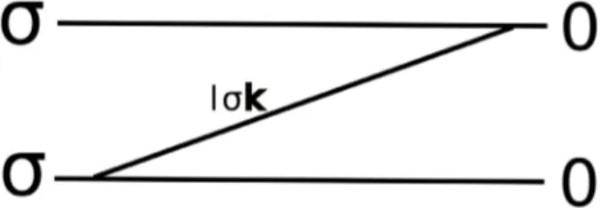
Fig. 1. An example of a second order diagram; by convention we let the time increase from the right to the left. The hori- zontal lines are calledcontours, the third linetunneling line; it represents an electron from leadl with spinσ and wave vec- torkwhich tunnels in two steps onto the dot. The intersection points of the tunneling lines with the contours are called ver- tices. The vertices separate the contours into intervals, and to each of these we assign a quantum dot state. The particle num- ber of neighbouring quantum dot states can differ only by±1.
The chronological order of the density matrices of the quan- tum dot in this diagram, viewed still as a diagram in the time space, is found as follows: we imagine a vertical line which cuts each of the contours one time. We consider then especially the intervals between two neighbouring vertices which are cut by the vertical line and take the two quantum dot states assigned to them. If they are a and bon the lower and on the upper contour, respectively, then the current quantum dot matrix is given by|ab|. The imaginary vertical line we move from the right to the left end of the diagram. The sequence of quantum dot matrices in the above diagram is:|00|,|0σ|and finally
|σσ|.
equation (1), is analytic in the coupling parameter and its Taylor expansion up to the order 2nis obtained by taking into account the corresponding orders of the kernels.
3.2.1 Second order density matrix
One of the diagrams visualizing the second order contri- butions to the density matrix kernel is shown in Figure1.
A possible way of describing the process is to say that the quantum dot is at first in the unoccupied state 0; then an electron with spinσtunnels in two steps onto the dot.
Finally, the dot is in the state σ. The analytical expres- sions which correspond to the diagrams are given by dia- grammatic rules, e.g. [31,34,45,48]. The expression for the diagram in Figure1reads:
1
fl(εlkσ)|Tlkσ|2 λ+i(εlkσ−E10),
where we let λ, the argument of the Laplace trans- form, still be finite. For simplicity we assume degener- acy, Eσ=E¯σ, and writeEσ0 =:E10. Later, we will con- sider also the case of different energies Eσ = E¯σ. We let fl(ε) be the Fermi function at chemical potential μl
and temperature T, i.e. fl(ε) = f((ε−μl)/kBT) with f(x) = 1/(1 +ex). We perform then the sum with re- spect to the leads and the wave vector. The thermody- namic limit is taken by replacing the sum with respect to the allowed wave vectors k by an integral over the first Brillouin zone.
Fig. 2. Second order diagrams of this form ensure that the trace of K(λ)|aa|is always zero. Their contributions to the density matrix kernel amount to−
b=ab| {K(λ)|aa|} |b.
We split now the integration into two parts: first, we fix the band energy and integrate over the surface in the first Brillouin zone whereεlkσequals this band energy. In a second step, we integrate over the band energies [49].
There are two diagrams of second order which are contri- butions to the kernel element σ| {K(λ)|00|} |σ. They are given by the above diagram and by the one we get by mirroring this with respect to a horizontal axis. Their contributions are complex conjugate, so we have to take two times the real part of the above expression. In the limitλ→0 we obtain:
σ| {K(λ= 0)|00|} |σ=2π
l
α+l (E10), where we used the notationα+l(ε) =αl(ε)fl(ε) and
αl(ε) =
{εlkσ=ε}
dSZl|Tlkσ|2
|∇εlσ(k)| . (3) Zl is the number of allowed wave vectors in the first Brillouin zone per volume in the wave vector space. In the case that the tunneling coefficientsTlkσwere indepen- dent of the wave vector, the function αl(ε) would just be proportional to the density of electron levels in leadl[49].
The other second order kernel elements are calculated essentially in the same way. With the further notation α−l (ε) =αl(ε)(1−fl(ε)) we obtain:
0| {K(λ= 0)|σσ|} |0= 2π
l
α−l (E10), 2| {K(λ= 0)|σσ|} |2= 2π
l
α+l (E21), σ| {K(λ= 0)|22|} |σ= 2π
l
α−l (E21).
For simplicity we assume for this that the definition ofαl, equation (3), does not depend on the spin. By considering the contributions of diagrams as in Figure2one can ver- ify that the general property of the density matrix kernel Tr{K|aa|}= 0 holds true alsowithin the second order theory. Therefore, we already calculated implicitly the re- maining kernel elements of the forma| {K(λ)|aa|} |a.
In all situations considered in this text the density ma- trix kernel maps a diagonal matrix to a diagonal matrix,
i.e.b| {K(λ= 0)|aa|} |b= 0 ifb=b. Thus, it is a lin- ear operator with rank three or lower acting on the four dimensional space of the diagonal matrices, since one de- gree of freedom is destroyed by the condition that the trace of the resulting matrix is zero. We can conclude that there is a diagonal solution ρof the quantum master equation (QME) in the stationary limit. With the notations
ρaa:=a|ρ|a, Γl,01± := 2π
α±l (E10) and Γ±l,12:= 2π
α±l (E21)
the QME turns into the following set of two equations for the three variablesρ00, ρ22 andρ↑↑ =ρ↓↓:
0 =−ρ00
l
Γl,01+ +ρσσ
l
Γl,01− , 0 =ρσσ
l
Γl,12+ −ρ22
l
Γl,12− .
This information is sufficient to determine the stationary reduced density matrix since we know that the normaliza- tion condition,ρ00+2ρσσ+ρ22= 1, holds. The solution is:
⎛
⎜⎝ ρ00
ρ↑↑
ρ↓↓
ρ22
⎞
⎟⎠= 1 Γ12−Γ01+Γ01+Γ12
⎛
⎜⎜
⎝ Γ01−Γ12− Γ01+Γ12− Γ01+Γ12− Γ12+Γ01+
⎞
⎟⎟
⎠, (4)
where we used the notations Γab±:=
l
Γl,ab± , Γab:=Γab++Γab−.
3.2.2 Second order current kernel
In order to calculate the current we have to determine the second order current kernel. The structure of the contri- butions to it is the same as that of the contributions to the density matrix kernel. We take into account only the diagrams with the final vertex on the lower contour. The lead index attached to the corresponding tunneling line is fixed and given by the lead onto which we are calculat- ing the current. An additional sign, as compared to the density matrix kernel, has then to be taken into account.
There are several equivalent possibilities of defining the current kernel [44].
The second order particle current is found by apply- ing the current kernel to the reduced density matrix and taking the trace [31]:
Il(2)= 2 N
Γ12− Γ01+
Γ¯l,01+ Γl,01−Γ¯l,01Γl,01+ Γ¯l,12Γl,12− −Γ¯l,12− Γl,12
, (5)
where we used ¯l to denote the opposite lead of leadl and the abbreviations:
N :=Γ12−Γ01+Γ01+Γ12, Γl,ab :=Γl,ab+ +Γl,ab− .
This is the particle current onto lead l. The net current, i.e. the sum of the two currents onto leadland ¯l, is zero.
In the case of proportional tunneling coupling, i.e. αl=κlα, with κl positive scalar factors fulfilling
lκl= 1, the expression for the current can be simplified:
Il(2) = 2 1 +ΓΓ01+Γ12
01Γ12−
κlΓ¯l,01+ −κ¯lΓl,01+
+ 2
1 + ΓΓ01+Γ12− 01Γ12
κ¯lΓl,12− −κlΓ¯l,12−
. (6)
The prefactor of the second line turns out to be the sta- tionary electron number on the quantum dot, i.e. the ex- pectation value Tr{Nρ} withN the particle counting operator on the quantum dot; the prefactor of the first line is the expectation value of 2−N, and we refer to it as the hole number.
Our non-perturbative approximation (DSO) is an ex- tension of the second order theory. The equations for the density matrix and the current in terms of the transition ratesΓl,ab± still hold true but the expressions for these rates change.
4 Dressed second order diagrams
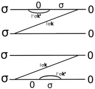
In this section we account for diagrams similar to the ones of the second order theory but dress them by charge fluctu- ations. Figure3shows two possibilities of dressing the sec- ond order diagram of Figure1. There is one more electron level of the leads involved in the tunneling processes given by these diagrams. We might comment that an electron (lower example diagram) or a hole (upper example dia- gram) tunnels for some time halfway onto the dot and then leaves it again. The tunneling of the one electron which finally enters the dot is accompanied by the tunneling of further electrons or holes in these diagrams.
According to the diagrammatic rules the sum of the contributions of the diagrams in Figure 3 to the density matrix kernel is given by:
1
dε α+(ε) λ+i(ε−E10)
× −1
λ+i(ε−E10)
dε α(ε) λ+i(ε−ε), where we letλstill be finite and used the notations:
α±:=
l
α±l ,
α:=α++α−=
l
αl.
Fig. 3.Two examples of dressing the diagram of Figure1with further tunneling lines. In the upper diagram the temporal se- quence of quantum dot matrices is: |00|,|0σ|,|00|,|0σ|
and |σσ|. A hole from leadl with wave vectork is partic- ipating in the process. In the lower diagram, it is a further electron which is accompanying the tunneling of the electron from the levellkσ.
Fig. 4.The existence of the state 2 leads to a fourth possibility of dressing. The tunneling line on the upper contour represents an electron of the opposite spin which tunnels onto the dot and leaves it again.
In the first line we recognize the contribution of the second order diagram. However, the integrand is multiplied by a factor, the second line, and this reflects the participation of further particles. From the upper diagram in Figure 3 we getα−(ε), from the lower one we getα+(ε). The sum yieldsα(ε), which appears in the factor.
Because of the existence of the two spins there is still a third way of dressing our second order diagram with one further tunneling line: thebubble on the lower contour of Figure3might as well represent an electron withopposite spin which accompanies the tunneling. The contribution of this diagram is the same as the contribution of the diagram with only one spin appearing, but it is important because it does not have a counterpart: there isno way of dressing the diagram with a bubble on the upper contour which represents a hole of the opposite spin. Finally, there is the possibility to dress the diagram by a tunneling line on the upper contour which represents an electron of the opposite spin, as shown in Figure4.
We saw that there are four ways of dressing the second order diagram with one bubble. Moreover, we can dress the diagrams with two or even more, in
Γl,01± =2π
dε α±l (ε)
(α+α+)(ε) +α+(E20−ε) π2[(α+α+)(ε) +α+(E20−ε)]2+
ε+pα+α+(ε)−pα+(E20−ε)−E102, (8)
Γl,12± =2π
dε α±l(ε)
(α+α−)(ε) +α−(E20−ε) π2[(α+α−)(ε) +α−(E20−ε)]2+
ε+pα+α−(ε)−pα−(E20−ε)−E212, (9)
Fig. 5. An example of a diagram with four bubbles. If we count the bubbles from the right to the left, then for the choice of each of them we have four different possibilities. This example-diagram contains all four of these possibilities.
generaln, subsequent, non-intersecting bubbles. An ex- ample is sketched in Figure 5. For the choice of each of these bubbles we have four possibilities. It might represent an electron of the same or the opposite spin and thus ap- pear on the lower contour, or represent a hole of the same spin or an electron of the opposite spin and appear on the upper contour. The sum of the contributions of all of these diagrams to the kernel element σ| {K(λ)|00|} |σis
1
dε α+(ε) η+i(ε−E10)
∞ n=0
−1 η+i(ε−E10)
n
×
dε(α+α+)(ε)
η+i(ε−ε) + α+(ε) η+i(ε+ε−E20)
n
=
dε α+(ε)/
η+i(ε−E10) +
dε(α+αη+i(ε+−)(εε))+η+i(ε+εα+(ε−)E
20)
, (7) where we replaced λby η. In Appendix A we sketch a proof of the equality for arbitraryλ∈ {Re >0}.
4.1 DSO tunneling rates
All of the other second order diagrams can be dressed in the same way. For the diagrams connecting the particle numbers one and two we see that a support of the tunnel- ing by holes and electrons of the same spin and by a hole of the opposite spin is possible, but not by an electron of the opposite spin. We obtain the following transition rates within this dressed second order approximation:
see equations(8) and (9)above,
where we define for any functionhthe functionphby:
ph(ε) :=
∞
0
dωh(ε+ω)−h(ε−ω)
ω ; (10)
ph(ε) is a principal part integral.
Hence, the DSO rates are given in the form of an inte- gral where the integrand is the product of the second order functions α±l (ε) and of a Lorentzian-like resonance func- tion. We, thus, expect that the second order rates are re- covered when the temperature broadening of the functions α±l largely exceeds the width of the Lorentzian broaden- ing. In the regimekBT 2πα(EF) these transition rates indeed turn into the transition rates of the second order theory.
The stationary reduced density matrix within the DSO is given by equation (4) and the current is given by equation (5) and in the case of proportional coupling by equation (6).
4.2 Linear conductance within the DSO
We assume that the second order functions αl, equa- tion (3), are obtained by multiplication of the density of electron levels in the leads by a coupling constant, and assume a simple shape of the density of electron levels, Figure7.
Deriving the formula for the current, equation (6), with respect to the bias,eVbias =μl−μ¯l, one obtains at zero bias the following expression for the linear conductance:
see equation(11)next page
where EF is the Fermi level, f(x) = 1/(1 +ex) the normalized Fermi function,
n= 2 1 +ΓΓ01+Γ12−
01Γ12
is the particle number on the dot as noted above, and where we use the abbreviations d01(ε) and d12(ε) for the denominators in the expressions for the transition rates, equations (8) and (9), respectively. The prefactor 4κlκ¯lis one in the case of symmetric coupling and less than one otherwise. We finally included the electron charge in the formula.
5 Result of the DSO for a spinless quantum dot
We consider here the case of a spinless quantum dot with only two possible states 0 and σ, so with only one spin.
This problem is equivalent to the SIAM with E↑ = E↓ andU = 0 in the sense that the current across the SIAM
GDSO= 4κlκ¯l
e2 h
(2−n)|Vbias=0 n|Vbias=0
⎛
⎜⎜
⎝ dε π
2α(ε)[(α+α+)(ε)+α+(E20−ε)]
d01(ε)
Vbias=0k−1BTf ε−EF
kBT
dε π2α(ε)[(α+α−)(ε)+α−(E20−ε)]
d12(ε)
Vbias=0k−1BTf ε−EF
kBT
⎞
⎟⎟
⎠ (11)
Fig. 6. The structure of the diagrams within the RTA. They are defined by the condition that any vertical line cuts at most two tunneling lines. When projecting all of the vertices of two- contour diagrams (see previous figures) onto one contour only, then any RTA diagram has the structure sketched in the figure:
there is an integer number of neighbouring “long” tunneling lines with an overlap of one vertex. Moreover, in the intervals enclosed by the long tunneling lines there can be an arbitrary number of bubbles. For the sum of all of these diagrams an integral equation was derived [34]. Its origin is the relation between the contributions of all RTA diagrams with nor less long tunneling lines on the one hand and of all RTA diagrams withn+ 1 or less long tunneling lines on the other hand. In the limitn→ ∞the two are equal.
quantum dot is then just two times the current across a spinless quantum dot.
The resonant tunneling approximation (RTA) is the diagram selection defined by the condition that any imag- inary vertical line cuts at most two tunneling lines [31,34].
It has been applied to the case of the spinless quan- tum dot, in which it is exact [50], to the case of in- finite interaction [31], but also to the case of finite interaction [35,36]. The structure of the RTA-diagrams is conveniently sketched by projecting all vertices onto one contour only (Fig.6).
The DSO takes into account only diagrams with the structure of the first line of Figure 6. In the cases of the spinless quantum dot and of the Anderson model with in- finite interaction, the DSO takes into accountalldiagrams with the structure of the first line of Figure6. In the case of finite interaction, on the other hand, the DSO does not contain all diagrams with the structure of the first line.
Unlike the DSO, the diagram selection defined by the first line in Figure 6 yields the exact result for the current in the limit of vanishing interaction.
The tunneling rates obtained by the DSO in the spinless case are:
Γl,01± = 2π
dε (α±l α)(ε)
π2α2(ε) + (pα(ε) +ε−E10)2.
We get the density matrix ρ00
ρ11
= 1
Γ01++Γ01− Γ01−
Γ01+
and the particle current in the case of proportional coupling:
IlDSO= 4κlκ¯lπ2 h
dε α2(ε) (f¯l−fl) (ε) π2α2(ε) + (ε+pα(ε)−E10)2· In the limit of small temperatures and in case the second order functions αl(ε) are rather constant, the current is obtained by integrating a Lorentzian-like function with width (full width at half maximum) Γ := 2πα between the two chemical potentials. The differential conductance as function of the bias thus reproduces the shape of this Lorentzian. Frequently, the quantity Γ rather than α is used to define the coupling.
In the case of proportional tunneling coupling the re- sult of the DSO for the spinless quantum dot is actually the same which was presented within the RTA [34] and thus exact.
We will now concentrate on applying the DSO approxi- mation to cases with nonzero interaction. We will consider the regimes Γ ∼ kBT and Γ kBT and ask with re- spect to which aspects the DSO is successful in explaining experimental results and how it compares with existing theories.
6 The case of infinite interaction
In the case of infinite interaction, U = ∞, all of the di- agrams which contain the state 2 are neglected and the equality ρ00+
σρσσ = 1 holds. The formulas for the linear conductance of the RTA [31] and DSO in the case of infinite interaction read:
GRT A= 4κlκ¯le2 h2
×
dεπ2α2(ε) d(ε)
−1 kBTf
ε−EF
kBT
, GDSO = 4κlκ¯le2
h (2−n)
×
dεπ2[α(α+α+)] (ε) d(ε)
−1 kBTf
ε−EF
kBT
, where we used the abbreviation
d(ε) :=π2(α+α+)2(ε) + (ε+pα+α+(ε)−E10)2
Fig. 7. Energy dependence of the dimensionless function b(ε) =α(ε)/α(EF). We placed the Fermi levelEF in the mid- dle in order to ensure that the chemical potential at equilibrium always equals the Fermi level. Moreover, we choseW = 1 eV, w= 0.9 W. A cut-off is needed in order to ensure the existence of the principal partspα, pα+, etc. of equation (10).
for the common denominator. Differences are only found in the prefactor and in the numerator. To compute the conductances we have to make a choice about the second order function α(ε). We wrote α(ε) = α(EF)b(ε) with a dimensionless function b(ε) fulfilling b(EF) = 1. The variable α(EF) is then our coupling parameter. Figure 7 shows how we chose the functionb(ε).
6.1 Coulomb peaks from high to low temperatures In Figure8we compare the linear conductances as a func- tion of the gate voltage obtained within the RTA and the DSO for various temperatures. We observe a tran- sition from a temperature dominated to a tunneling dom- inated width of the Coulomb peak. The transition occurs at temperatures around 1 K which corresponds to a ther- mal energy which is of the order of the chosen coupling α(EF) = 0.042 meV. The peak height of the DSO still increases up to temperatures of about 100 mK and de- creases then. In this respect, the DSO fails to describe ex- perimental reality below 100 mK. Notice that the shape of the curve saturates at low temperatures both within the RTA and the DSO: the effect of decreasing the tempera- ture further and further is only a shift of the graph. As we will show in the next subsection and in Appendix B, these features do not depend on the choice ofb(ε).
6.2 Universality and Kondo temperature in the infinite U-case
We show now that the DSO conductance displays uni- versality as function of the temperature in the regime of strong coupling. For a fixed value of the gate voltage, i.e.
for fixedE10, the linear conductance becomes a function
Fig. 8. Linear conductance of the DSO as a function of the energy difference E10 for different temperatures. The dashed lines show the result of the RTA; the coupling we chose to be α(EF) = 0.042 meV and W = 1 eV (the same choices we made for a later comparison with an experiment, discussed in Sect.7.2). A temperature of 1 K corresponds to a thermal energy of about kBT ≈0.1 meV. For large temperatures the resonance is smeared out, its centre is found roughly around the Fermi level. For decreased temperatures the position of the maximum is shifted and the width of the peak is propor- tional toα(EF). While the logarithmic shift of the peak with the temperature does not stop, the shape of the curve and its maximum value saturate. We find numerically within the RTA the maximum≈0.99e2/h, within the DSO≈0.69e2/h. We em- phasize that neither these maximum values nor the shapes of the curves in the limit of small temperatures depend on the the way in which the functionb(ε) is chosen.
G(T) of the temperature. This is expected to display uni- versality [51] in the following sense: there is a tempera- ture TK such that G(T)/Gmax is a universal function of the ratioT /TK, whereGmax is the maximum value of the conductance. We can show that this holds for GRT A as well as for GDSO in case E10 EF. Both the RTA and the DSO, however, do not yield the expected convergence G(T)→Gmax= 4κlκ¯l2e2/h(T→0).
We present in Appendix B a derivation of the univer- sality of the conductance obtained by the DSO and the RTA, respectively. For the temperature TK, defined by the condition that the conductance reaches one half of its maximum, we obtain:
kBTK= 7Wexp
E10−EF
α(EF)
. (12)
The prefactor 7 changes if the shape of the band (Fig.7) is chosen in a different way, for example, to be Lorentzian.
The conditions under which the results of Appendix B are valid read:
kBT α(EF)W.
In this case we obtain the expression GDSO = 4κlκ¯le2
h(2−n)FDSO
c1/2+ log T TK
, where TK is given by equation (12), n is the par- ticle number and the function FDSO is defined in equation (B.7) (Appendix B).
Γlσ±= 2π
dε α±l (ε)
α(ε) +α+(ε+Eσσ¯ )
π2(α(ε) +α+(ε+E¯σσ))2+ (ε−Eσ0+pα(ε) +pα+(ε+Eσσ¯ ))2 (13)
Fig. 9.A comparison of the universal function of the DSO with an NRG-fit [7]: both functions take the value 0.5 at T =TK
and are normalized in such a way that the maximum is one.
A striking feature of the fit is that within one power of ten the linear conductance increases from 50% to about 95% of its maximum while our function is growing much less in this interval. We included also the universal curve which is obtained for the RTA. In agreement with Figure8and unlike the NRG- fit, the universal functions of RTA and DSO decrease again for even smaller exponents than shown here. The equation for the NRG-fit isG(T) =Gmax
1/
(T /TK )2+ 1s
withTK = TK/(21/s−1)1/2 so thatG(TK) =Gmax/2; we choses= 0.2.
The particle number n is in general a function of temperature and gate voltage. At temperatures kBT α(EF) and whenE10 EF (compared to the coupling), however,nessentially becomes a constant, since the elec- tron is then trapped in the dot. The DSO linear conduc- tance becomes a universal function ofT /TKin the regime E10EF; atT =TK,G(T) reaches one half of its maxi- mum. In Figure9we compare our result for the universal function with a fit to the one obtained by NRG calcula- tions [51]. The same reasoning one can apply to the RTA in order to obtain an analogous universality; the result- ing formula for TK deviates only in the prefactor. The relation betweenα(EF) and the coupling parameterΓ by the use of which TK is most frequently expressed, e.g.
references [7,29,44], isΓ = 2πα(EF).
We acknowledge very clearly that the DSO fails to de- scribe the regime of strong coupling quantitatively cor- rectly. For example, the DSO (and the RTA) expression forTK, given in equation (12), has an exponent which dif- fers by a factor of two from the exponent extracted from more accurate theories [5]. However, we think it is very remarkable that the linear conductance obtained by it dis- plays a universality in the same sense as it is predicted by perfectly different approaches.
6.3 Zero bias anomaly of the differential conductance In addition to the linear conductance we considered the differential conductance obtained within the DSO for in-
Fig. 10.The differential conductance versus the bias. We set E(0)10 =EF−1 meV and choseα(EF) = 0.042 meV,W = 1 eV as in Figure8. We fixed one of the chemical potentials at the Fermi level, μl0 = EF, changed only the other one and de- fined eVbias = μl¯0 −EF. We assumed a capacitive coupling between the leads and the quantum dot in such a way that E10(Vbias) =E(0)10 + 0.2eVbias. We see a resonance appearing at zero bias for small temperatures. The dashed lines show the result of the RTA. The resonance is becoming more and more pronounced with decreasing temperature. The shape of the curve depends on the capacitive coupling and on how the window between the two chemical potentials is opened; how- ever, the appearing of the zero bias anomaly does not in prin- ciple depend on these choices as one can conclude from the fact that they are irrelevant for the differential conductance at zero bias.
finite U. We notice that in qualitatively the same way as the RTA [31] the approximation produces a zero bias maximum of the differential conductance in case E10 lies below the Fermi level (Fig. 10) and a minimum in case it lies above or in the vicinity of the Fermi level. The effect becomes more pronounced for smaller and smaller temperatures.
The generalization of the DSO for infinite U to the case of different energiesE↑ =E↓ is straightforward. One obtains the tunneling rates
see equation(13)above.
We see (Fig. 11) that the zero bias anomaly is split ac- cording to eVbias ≈ ±E↑↓, in agreement with theoretical results [28,31,52,53] and experiments [8,30,54].
6.4 Situations in which only one resonance is expected In reference [8] a resonance close to zero bias whose posi- tion changed slightly with the gate voltage was reported.
The dependence of the position on the gate voltage was explained by the conjecture that two different wave func- tions (not only two different spins) might be involved, so


![Fig. 9. A comparison of the universal function of the DSO with an NRG-fit [7]: both functions take the value 0.5 at T = T K](https://thumb-eu.123doks.com/thumbv2/1library_info/5656010.1694181/11.892.78.685.134.430/fig-comparison-universal-function-dso-nrg-functions-value.webp)


