Determination of the Column Density in the KATRIN Beamline with

Technische Universität München Fakultät für Physik

Master's Thesis

Determination of the Column Density in the KATRIN Beamline with

Electrons from the Photo-Electric Source

Christoph Köhler

09. December 2019

Supervisor: Christian Karl

Declaration of Authorship

English:

I hereby declare that I am the sole author of this master’s thesis and that it was written independently only using the cited external resources.

German:

Ich erkl¨ are hiermit, dass die vorliegende Masterarbeit von mir selbstst¨ andig verfasst wurde und dass keine anderen als die angegebenen Quellen und Hilfsmittel benutzt wurden.

Christoph K¨ ohler

Munich, 09.12.2019

Abstract

The Karlsruhe Tritium Neutrino (KATRIN) experiment currently provides the best limit on the effective electron antineutrino mass of all the experiments that use the direct method of observation to m _ν < 1.1 eV (90 % C.L.). It is designed to measure m _ν with a sensitivity of 200 meV (90 % C.L.) within 5 years of operation. To achieve this goal a strong reduction of statistical and systematical uncertainties is required. One important model parameter in the KATRIN experiment is the column density, that has to be determined with a precision of 0.2 %.

In this thesis different ways to obtain the column density were studied in detail. The most precise technique makes use of an angular resolved electron gun installed at the rear- end of the KATRIN beamline. In this thesis the analysis to infer the column density from the e-gun data was developed. To this end, a model of the KATRIN response function for e-gun electrons and the parameter inference based on the covariance matrix technique was implemented in the KATRIN analysis software Fitrium. This method was successfully applied for the first neutrino mass science run of KATRIN.

As the e-gun calibration is only performed on a weekly basis, means to determine the column density in between the e-gun calibrations during each beta-scan have to be found.

To this end, the Beta Induced X-ray Spectrometry, Forward Beam Monitor and flowmeter sensor data was analyzed and a method to extract run-wise ρd values and uncertainties developed.

Furthermore, a study was performed to optimize the measurement time distribution of

the column density determination with the photo-electron source. This thesis is concluded

with an analysis of the first science run data, with a special focus on the correlation of the

column density on the other parameters of interest, such as the neutrino mass and endpoint.

Contents

1 Neutrinos in the Standard Model of particle physics and beyond 1

1.1 Postulation and discovery . . . . 1

1.2 Standard Model description . . . . 2

1.3 Neutrino Oscillation . . . . 2

1.4 Mass Determination . . . . 3

1.4.1 Cosmology . . . . 4

1.4.2 Neutrinoless Double β-Decay . . . . 4

1.4.3 Single β-Decay . . . . 5

2 The KATRIN Experiment 7 2.1 MAC-E-Filter . . . . 7

2.2 Experimental setup . . . . 9

2.2.1 Source and transport section . . . . 9

2.2.2 Spectrometer and detector section . . . . 13

2.3 Model of the integral β-spectrum . . . . 14

2.3.1 Differential Decay Spectrum . . . . 14

2.3.2 Response function . . . . 15

2.3.3 Integral β-spectrum . . . . 17

3 Column density monitoring devices 18 3.1 Column density stability . . . . 18

3.2 Photo-electron source . . . . 18

3.3 Beta Induced X-ray Spectrometry . . . . 20

3.4 Tritium loop sensor . . . . 21

3.5 Forward Beam Monitor . . . . 22

3.6 Focal Plane Detector . . . . 23

4 Determination of ρdσ with the photo-electron source 24 4.1 Response model . . . . 24

4.1.1 Transmission function . . . . 25

4.1.2 Energy distribution . . . . 25

4.1.3 Angular distribution . . . . 27

4.1.4 Response function . . . . 27

4.2 Measurement principle . . . . 28

4.3 Fitting strategy . . . . 29

4.4 Determination of ρdσ during KNM-1 . . . . 30

4.4.1 Photo-electron measurement . . . . 30

4.4.2 Systematic effects . . . . 31

4.4.3 ρdσ fit . . . . 32

5 Stability of the column density during KNM-1 36 5.1 Continuous ρdσ monitoring . . . . 36 5.2 Systematic uncertainty . . . . 37

6 ρdσ measurement time optimization 40

6.1 ρdσ measurement . . . . 40 6.2 Nominal KATRIN setting . . . . 41 6.3 First neutrino mass measurement . . . . 42 7 Column density as an additional free fit parameter 45 7.1 ρdσ determination from data . . . . 45 7.2 Parameter correlation . . . . 45

8 Conclusion 49

Chapter 1

Neutrinos in the Standard Model of particle physics and beyond

The neutrino is one of the greatest remaining mysteries in the world of particle physics.

Its existence was first postulated theoretically. Being a lepton without electric charge and interacting only weakly, it took 30 years to be discovered in an experiment. Despite many discoveries ever since, the neutrino remains one of the least understood particles of the Standard Model. Among other open questions its absolute mass is still unknown.

This chapter is structured in the following way: In section 1.1 there is first given a brief summary of the history of the neutrino, followed by its theoretical description in the Standard Model in section 1.2. The recent discovery of neutrino oscillation is addressed in section 1.3 and the last section 1.4 is devoted to the neutrino mass determination.

1.1 Postulation and discovery

At the beginning of the 20 ^th century studying the β-decay of atomic nuclei J. Chadwick made an unexpected discovery. Unlike the discrete lines in α- and γ-decay, he observed a continuous energy spectrum for the emitted electrons [Cha14]. At this time the β-decay was thought to be a two-body decay with the emission of a proton and an electron. Both particles would always receive the same amount of energy in the decay, which stood in contrast to Chadwick’s observation. A solution to this problem was proposed by W. Pauli in his famous letter to a group of physicists in 1930, where he postulated the existence of a neutral spin-

1

2 particle that is emitted together with the electron in the β-decay [Pau30]. By sharing the energy released in the decay between this new particle and the electron the continuous spectrum could be understood. Further motivation for this postulation arose from the fact, that for angular momentum conservation additional spin was needed, which then would be provided by the new particle [Zub11].

After the discovery of the neutron only short time later E. Fermi was able to describe the β-decay in detail in his successful theory [Fer34]. The underlying reaction was now understood to be a three-body decay:

n → p ⁺ + e ⁻ + ¯ ν _e (1.1)

More than 20 years after its postulation the existence of the neutrino was proven by Cowan and Reines in an experiment that was performed at Hanford in 1953 [CRH+56].

They used nuclear reactors as the source of an intense neutrino flux and observed the signal that arises from the reaction of an electron antineutrino with a proton, shown in eq. (1.2).

¯

ν _e + p ⁺ → e ⁺ + n (1.2)

Combining a large water tank with dissolved CdCl ₂ with an additional liquid scintillator they could observe a very characteristic delayed pulse pair that is created by the reaction products.

First, the positron annihilates with an electron resulting in the emission of 511 keV photons, which is then followed by the moderated neutron being captured on cadmium releasing a second pulse of photons

n + ¹¹³ Cd → ¹¹⁴ Cd + γ. (1.3)

The liquid scintillator detects both the photons from the positron annihilation and the neu- tron capture and hence the time-delayed spectrum could be studied in detail. To further confirm that the detected signals originated from reactor neutrinos interacting with the pro- tons in the water tank, the signal rate was compared to the one expected from the reactor output. In this way, despite the large background of the experiment stemming from cosmic radiation, Cowan and Reines could conclude that they had detected neutrinos for the first time [CRH+56].

1.2 Standard Model description

The Standard Model of particle physics is a theory describing the interactions between fun- damental forces and elementary particles [Pov+15]. It comprises three of the four known fundamental interactions: the strong, the weak and the electromagnetic force. It was devel- oped by a large group of scientists in the second half of the 20th century and successfully predicted the existence of many new particles. However, the theory does not yet include the gravitational force and it cannot explain certain phenomena in particle physics, such as the observation of neutrino oscillation. This means that the Standard Model needs to be extended in order to cover all of the aspects of particle physics.

In the SM neutrinos are described as leptons without electric charge. Therefore they undergo only weak interactions. Experiments have proven that neutrinos violate parity. To explain this result the V–A theory of weak interaction was developed. Furthermore, the study of the charged pion decay implies that the electron neutrino is different from the muon neutrino [Pov+15]. The total number N ν of light neutrinos was determined to be three by measuring the decay width of the Z ⁰ resonance [Zub11]. Neutrinos therefore exist in three different flavors that can be associated to each lepton family respectively:

ν e

e ⁻

ν µ

µ ⁻

ν τ

τ ⁻

In the Standard Model description neutrinos are assumed to be massless. However in 1998 by discovering neutrino flavor oscillation it was shown that this assumption is not valid [FHI+98]. The fact that neutrinos have mass is to this date the only testable evidence of physics beyond the Standard Model and it makes the study of neutrino parameters so interesting [Pov+15].

1.3 Neutrino Oscillation

The first theoretical descriptions of neutrino oscillation were formulated in mid of the 20 ^th

century by Pontecorvo, who predicted the possibility of neutrino-antineutrino oscillations

[Pon68], and by Maki, Nakagawa and Sakata, who proposed a two flavor neutrino mixing

1.4 Mass Determination

[MNS62]. The underlying requirement for these theories is that the neutrino flavor eigen- states differ from their mass eigenstates. The relation between them can be expressed via the so-called PMNS matrix



 ν _e ν µ

ν _τ



 =





U _e1 U _e2 U _e3 U µ

U µ

U µ

U _τ

U _τ

U _τ







 ν ₁ ν 2

ν ₃



 (1.4)

named after Pontecorvo, Maki, Nakagawa and Sakata. The matrix is parameterized by three mixing angles and one phase factor ¹ . Assuming for simplicity the case of only two neutrino generations reduces eq. (1.4) to

ν _e ν _µ

=

cos θ sin θ

−sin θ cos θ

ν ₁ ν ₂

. (1.5)

In this case the mixing can be describe by only one parameter the mixing angle θ. Taking the electron neutrino as an example, it can now be expressed as a superposition of the mass eigenstates ν 1 and ν 2

|ν _e i = cos θ |ν ₁ i + sin θ |ν ₂ i (1.6) The oscillation probability of the electron neutrino can in this case be written as:

P (ν _e → ν _µ ) = sin ² (2θ) sin ²

∆m ² L 4E

(1.7) One can see that the probability for oscillating into ν _µ depends on the mixing angle θ, the squared neutrino mass difference ∆m ² , the distance the electron neutrino has traveled L and its energy E. By measuring this probability in experiments at different distances and neutrino energies the mixing angle and the squared neutrino mass difference can be determined.

First experimental indication for neutrino oscillation was found in the 1960s by R. Davis and his group at the Homestake experiment. Using a chlorine-based detector they measured the flux of solar electron neutrinos. The comparison with the theoretical prediction showed a significant deficit which soon became known as the solar neutrino problem [CDD+98].

In 1998 Super-Kamiokande was the first experiment to directly observe the oscillation of neutrinos, by studying the composition of the atmospheric neutrino flux and comparing it to the predicted value. The discrepancy between prediction and observation could only be explained by oscillation of ν _µ to ν _τ [FHI+98].

The second direct evidence for neutrino flavor transformation was found in the Sudbury Neutrino Observatory (SNO) experiment. Here, in contrast to the Homestake experiment they could additionally observe neutral current interactions and therefore prove, that the total flux of solar neutrinos, consisting of all three flavors matches the theoretical predictions.

The solar neutrino problem could now be understood as the oscillation of ν e to ν µ or ν τ

[AAA+02].

1.4 Mass Determination

The phenomenon that neutrinos can oscillate implies that they have a non-zero mass. While the squared mass differences between the three mass eigenstates can be determined in oscil- lation experiments, the absolute value has to be obtained with other experiments.

1

Two additional complex phases are needed in the case of Majorana neutrinos, discussed in section 1.4.2

1.4.1 Cosmology

One of the possible ways to access the neutrino mass is to study cosmological data. Be- cause neutrinos have a high number density, they played an important role in the structure formation of the universe. After decoupling they were still highly relativistic particles and thus had a large free streaming length. The structures in the universe that we observe today were formed by small density fluctuations that grew in size due to gravitational clustering.

The relativistic neutrinos acting as hot dark matter would mitigate this growth by washing out small scale structures. The strength of this effect depends on the neutrino mass. It is therefore possible to set an upper limit on the sum of neutrino mass eigenstates

m cos = X

i

m i (1.8)

by studying the cosmic microwave background anisotropy in combination with the observa- tion of large-scale structures. A recent combined analysis using this method constraints the neutrino mass to

m _cos < 0.12 eV (1.9)

as shown in [Agh+18]. This result, as well as the other limits on m _ν obtained from cos- mological studies depend strongly on the underlying data set and are only valid within the ΛCDM concordance model.

1.4.2 Neutrinoless Double β-Decay

In double β-decay (0νββ), two neutrons decay simultaneously into two protons under emis- sion of two electrons and two electron antineutrinos

2n → 2p + 2e ⁻ + 2¯ ν e . (1.10)

If the neutrino is a Majorana particle, meaning that it is its own antiparticle, neutrinoless double β-decay (0νββ) is possible. Similar to the double β-decay (2νββ) two simultaneous β-decays are happening in the same nucleus. However, instead of creating two neutrinos, one virtual neutrino is exchanged inside the nucleus. This yields into a double β-decay where no neutrino is emitted

2n → 2p + 2e ⁻ . (1.11)

The energy spectrum of the 0νββ would feature a sharp line at the endpoint because the two emitted electrons would receive the full decay energy [GP12]. The lifetime on the other hand depends on the effective Majorana neutrino mass

m _ββ =

X

k

U _ek ² m _k

(1.12) which contains all three neutrino mass eigenvalues and the electron neutrino elements of the PMNS matrix. Possible cancellations can arise due to complex CP-violating phases. In addition the lifetime also depends on the nuclear matrix element of the decay, which therefore has to be known with high precision.

So far no direct observation of neutrinoless double β-decay could be made. The best

upper limits on the neutrino mass could be determined in the GERDA experiment with ⁷⁶ Ge

to be m ββ < 0.15 - 0.39 eV [Bar18] and in the KamLand-Zen experiment using ¹³⁶ Xe to be

m _ββ < 0.09 - 0.24 eV [Bar18].

1.4 Mass Determination

1.4.3 Single β-Decay

One direct method to retrieve the absolute neutrino mass scale is the kinematic study of the single β-decay. The underlying reaction is

(A, Z) → (A, Z + 1) ⁺ + e ⁻ + ¯ ν e + Q. (1.13) Here, in a nucleus (A,Z) a neutron decays into a proton resulting in a daughter nucleus (A,Z+1) ⁺ with an electron, an electron antineutrino and the surplus energy Q being emitted.

In each decay Q is distributed in a way that the daughter nucleus receives a varying amount of recoil energy E rec while the remaining energy, which is called the endpoint energy E 0

E 0 = Q − E rec = E + E ν (1.14)

is being shared between the electron and the electron antineutrino. The electron receives the energy E and the electron antineutrino the energy E _ν . The maximal energy the electron can receive is therefore given by the difference between E 0 and the energy needed to create an electron antineutrino at rest. Studying the energy spectrum of the emitted electron one is able to retrieve information about the effective electron antineutrino mass

m _ν = s

X

k

|U _ek ² | · m ² _k , (1.15)

which is defined as the incoherent sum of the squared neutrino mass eigenvalues m _k . The differential spectrum depending on the electron energy E is given by

dΓ

dE = C · F (Z, E) · p · (E + m _e ) · (E ₀ − E) · p

(E ₀ − E) ² − m ² _ν · Θ(E ₀ − E − m _ν ). (1.16) In this equation the constant C is defined as

C = G ² _F · cos ² θ _C

2π ³ · |M _nuc | ² . (1.17)

It includes the Fermi constant G F , the Cabbibo angle θ C and the nuclear matrix element M nuc . F (Z, E) corresponds to the Fermi function

F (Z, E) = 2 π η

1 − exp(−2 π η). (1.18)

and the momentum and mass of the electron are given by p and m e [OW08; KBD+19].

Because the neutrino mass signal has only a small magnitude, the selection of the optimal β-isotope is of great importance. β-emitter with a low endpoint E 0 have a larger fraction of the total number of decays in the region near the endpoint. A short lifetime leads to a high activity and therefore to high statistics with a low amount of source material.

Tritium with an endpoint of ≈ 18.6 keV and a half life of 12.3 yr satisfies both requirements and hence is used in the Mainz and Troitsk as well as in the KATRIN experiment [KBB+05;

ABB+11; Ake+19].

Looking at the β-decay of tritium, the differential spectrum over the whole range of possible electron energies is shown in fig. 1.1a. According to eq. (1.16) the neutrino distorts the shape of the β-spectrum depending on the value of its the mass. The distortion near the endpoint for different neutrino masses is depicted in fig. 1.1b.

The current best limit on the electron antineutrino mass is m ν < 1.1 eV (90 % C.L.)

and was measured by the KATRIN experiment in 2019 [AAA+19].

2.5 5.0 7.5 10.0 12.5 15.0 17.5 Electron energy (keV)

0.00 0.25 0.50 0.75 1.00 1.25 1.50 1.75

Rel. rate (a. u.)

1e 13

(a) Shape of the spectrum for the whole energy range.

3.0 2.5 2.0 1.5 1.0 0.5 0.0

E - E 0 (eV) 0.0

0.2 0.4 0.6 0.8 1.0 1.2 1.4

Rel. rate (a. u.)

1e 20

m = 0 eV m = 1 eV m = 2 eV

(b) Impact of the neutrino mass on the spectral shape near the endpoint.

Figure 1.1: Differential spectrum of the tritium β-decay.

Chapter 2

The KATRIN Experiment

The KATRIN experiment currently provides the best limit on the neutrino mass of all the experiments that use the direct method of observation, see section 1.4.3. Its aim is to measure the neutrino mass with a sensitivity of 200 meV (90 % C.L.) probing the sub-eV neutrino mass scale. Like its predecessors the Mainz and Troitsk experiment it searches for distortions of the β-decay spectrum of tritium that are caused by a non-zero neutrino mass.

The KATRIN experiment is located in Karlsruhe, where the Tritium Laboratory Karlsruhe (TLK) provides the necessary amount of tritium with high purity that is needed for the operation of the experiment. The goal of improving the ν-mass sensitivity by one order of magnitude in comparison with the Mainz and Troitsk experiment requires a reduction in statistical and systematic uncertainties by a factor of 100 [AAB+05].

In this chapter first the underlying measurement principle of the KATRIN experiment is described in section 2.1. It is followed by a description of the main experimental components that are needed to perform this high precision experiment in section 2.2. The last part, section 2.3, addresses the theoretical model that describes the measured integral β-spectrum.

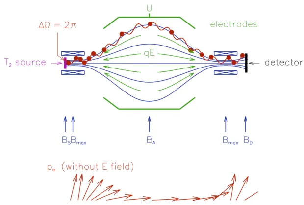
2.1 MAC-E-Filter

To measure the energy spectrum of electrons emitted in tritium β-decay very precisely the KATRIN experiment uses a method called MAC-E-Filter (Magnetic Adiabatic Collimation in combination with an Elecrostatic Filter). This technique consists of a new type of spectrom- eter that was first introduced by [BPT80]. Having a good energy resolution and providing a high luminosity at the same time this measurement principle was soon identified as a promising candidate to enhance the search for the neutrino mass in direct experiments. It was redeveloped independently for this purpose by the Troitsk and Mainz experiment [LS85;

PBB+92] and proved to be of great success.

The main tasks of the MAC-E-Filter consist of transforming the transversal energy E ⊥

of the electrons to energy in the parallel direction and providing an electric field that filters

out all the electrons with energies below a certain threshold. This transformation is of great

importance, since the electric field only acts in the longitudinal direction and therefore is not

able to influence or determine the transversal part of the electron energy. The experimental

components needed for this task together with an illustration of the electron momentum

change are depicted in fig. 2.1. The β-electrons that are created in the tritium source are

guided magnetically towards the spectrometer. Traveling with a cyclotron motion around the

magnetic field lines they can enter the MAC-E-Filter with solid angles up to 2π. To transform

their transversal energy the magnetic field acting upon them is continuously decreased from

a maximum value B max at the spectrometer entrance towards a minimal value B A at the

analyzing plane. This magnetic field gradient forces almost all of the transversal momentum

Figure 2.1: Illustration of the working principle of the MAC-E filter together with its exper- imental arrangement. Adapted from [AAB+05].

into the longitudinal direction. In case of adiabatic momentum transformation, which is valid here due to the slowly changing magnetic field, the magnetic moment µ stays constant:

µ = E ⊥

B = const. (2.1)

So by this technique the electrons that are created in the source by tritium decay are guided along the magnetic field lines through the spectrometer, where most of their transversal momentum is transformed into the longitudinal direction, and have to surpass a retarding potential in order to be reaccelerated and observed at the detector. Since for a given electric field only the electrons with an equal or higher energy can traverse the spectrometer, it acts as an integrating high-energy pass filter. Ideally it is desired to reduce all of the transversal electron energy. This is however not possible due to B _A > 0. From eq. (2.1) follows that the MAC-E-Filter has a finite energy resolution which is given by

∆E

E = B _A

B _max . (2.2)

In order to optimize the precision of the energy filter, the ratio between B _max and B _A should

be as large as possible. At the same time, to guarantee the adiabaticity of the magnetic field

the size of the spectrometer also has to become larger [AAB+05; KBD+19].

2.2 Experimental setup

2.2 Experimental setup

The aim of the KATRIN experiment to measure the neutrino mass with a sensitivity of 200 meV requires a significant reduction of the experimental uncertainties. Using the fully developed technology of the MAC-E-Filter and being provided with highly purified tritium by the TLK, the experimental configuration consists of a setup which is 70 meters long and is shown in fig. 2.2. The tritium gas is injected continuously into the windowless source and pumped out at both ends to ensure a constant amount of gas being present. On the rear side of this source a section equipped with calibration devices is situated. The task to guide the emitted β-electrons towards the detector and to reduce the amount of residual gas in the beamline is fulfilled by the transport section. Following, the pre-spectrometer filters out the lower energetic β-electrons, to reduce the background that could be induced by them in the main spectrometer. The detector at the end of the beamline measures the rate of the electrons that surpass both spectrometers.

Figure 2.2: The experimental configuration of KATRIN can be separated in: a) the rear section, containing instruments for diagnostics, b) the windowless gaseous tritium source WGTS, c) the transport section, which consists of a differential and a cryogenic pumping section, d) the pre-spectrometer, e) the main spectrometer and f) the focal plane detector (FPD).

In the following the main experimental parts of KATRIN are described in more detail, starting with the components that are related to the creation and transport of the β-electrons, described in section 2.2.1. The energy filtering and detection of the electrons is addressed in section 2.2.2.

2.2.1 Source and transport section

As we have seen in section 1.4.3 the imprint of the neutrino mass on the β-spectrum is strongest in the region near the endpoint. However, only a tiny fraction of the total β- decays produces electrons with this high energies. To perform a neutrino mass measurement with low statistical uncertainty requires therefore a strong β-electron source.

In the following the three components of the KATRIN experiment that are directly related to the tritium source are described.

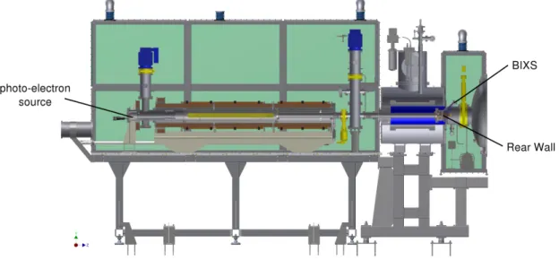
Rear Section

The rear section properly closes the WGTS on the rear side. For this task it contains a

differential pumping section, that pumps the remaining tritium gas into the Outer Loop of

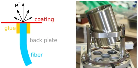
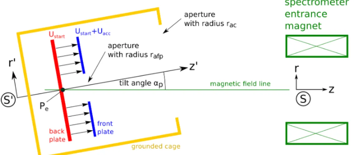
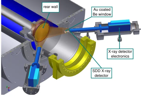
KATRIN. The rear end of the beamline is formed by the rear wall, a gold-plated stain-less steel disk, that absorbs the charged particles moving in this direction and ensures a well defined electrical potential over the full WGTS. Its location in the rear section is shown in fig. 2.3. A 5 mm wide hole in the wall enables the electrons from the photo-electron source, to pass into the beamline. By using an electromagnetic transport system, that includes steering coils in x- and y-direction, the electron beam is able to scan the whole flux tube area.

With this mono-energetic and angular-selective beam of electrons a variety of calibration measurements is possible. One of the main tasks of the photo-electron source, in the following also called electron gun, is to determine the column density ρd of the tritium source with high precision. Furthermore the study of the transmission properties of the MAC-E-Filter as well as the determination of the energy loss function are from great importance and can be achieved using this electron beam. A second calibration device monitoring the WGTS properties is located near the rear wall. It uses Beta Induced X-ray Spectrometry (BIXS) to monitor the activity of the WGTS. The β-electrons from the tritium decay are absorbed at the rear wall and create X-rays through bremsstrahlung. Measuring the intensity of these photons allows the observation of activity fluctuations of the gas in the WGTS [AAB+05;

Bab14; Beh16].

Figure 2.3: Illustration of the rear section setup. The rear wall terminates the beamline on this side. A small opening in the disk enables the electrons from the e-gun to pass into the beamline and with theses electrons dedicated calibration measurements can be performed. The BIXS detector monitors the activity of the sources by observing the emitted X-rays that are created when β-electrons reach the rear wall. Taken from [Bab14].

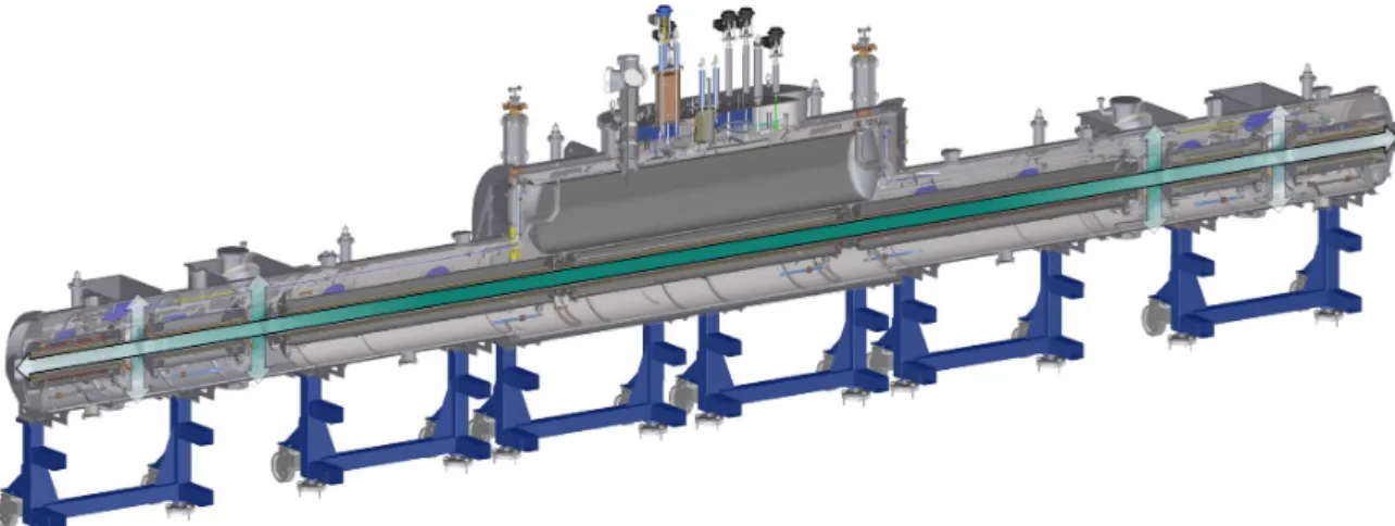
Windowless Gaseous Tritium Source

The tritium source of the KATRIN experiment consists of a windowless tube, where in the

center molecular tritium gas is injected. The gas is pumped out at both ends to form a

continuous circular flow of tritium. With this technique a constant gas column density of

5 · 10 ¹⁷ cm ⁻² can be achieved. In addition to providing this high column density the source

2.2 Experimental setup

Figure 2.4: A cross-sectional view of the 11 m long windowless gaseous tritium source (WGTS). Tritium is injected in the center and flows out at both ends of the beamline, where turbo-molecular pumps transport the tritium back into the loop system. The density profile of the tritium gas is indicated with the green color.

The β-electrons are guided magnetically to both sides, where they either enter the transport section or are absorbed at the rear wall. Taken from [Ha17].

needs to be stable on the per mille level.

Figure 2.4 displays the WGTS in an cross sectional view. The density of the tritium gas is indicated in the green color and allows the visualization of its flow inside the source.

The starting point of this loop system is the supply of molecular tritium gas with a purity of _T > 95 % by the TLK [AAB+05]. Once the gas is injected, its composition can be monitored continuously using laser Raman spectroscopy (LARA). A cryostat keeps the source tube and the contained tritium gas at a stable temperature of 30 K. This mitigates the effect of Doppler broadening, which is due to the relative motion between the tritium molecules and the beamline axis, and lowers the chance of leaving the daughter molecule of the β-decay in a highly excited final state [Mar17]. The nominal column density of 5 · 10 ¹⁷ cm ⁻² is close to the optimal, maximal value, that is limited by the increasing probability of the electrons to undergo inelastic scattering. Raising ρd above the maximal value does not increase the signal strength anymore [AAB+05]. After injection, the bulk of the tritium gas is retracted at both ends of the source tube with four turbomolecular pumps and fed back into the loop cycle. The probability of creating β-electrons follows the density profile of the gas along the beamline axis. The electrons itself are emitted isotropically, with the pitch angle θ describing the direction of the electron momentum with respect to the magnet field.

With this setup the source of the KATRIN experiment can create about 10 ¹⁰ β-decay

electrons per second. Using several superconducting magnets these electrons are guided along

the magnetic field lines towards the detector and the rear wall, respectively. Because the β-

electrons are emitted isotropically their path lengths inside the source differ in size. A longer

path increases the probability to undergo inelastic scattering. It is therefore favorable to

reject all electrons emitted with an angle above a certain value θ max . This can be achieved

by lowering the magnetic field inside the source according to the condition of magnetic

reflection, given in eq. (2.3).

sin θ _max = r B _S

B max

(2.3) To meet the KATRIN systematics budget the WGTS has to be operated with a stability on the per mille level in regard to the temperature and pressure inside the source. In addition the activity of the WGTS has to be monitored with high precision [Ha17; AAB+05].

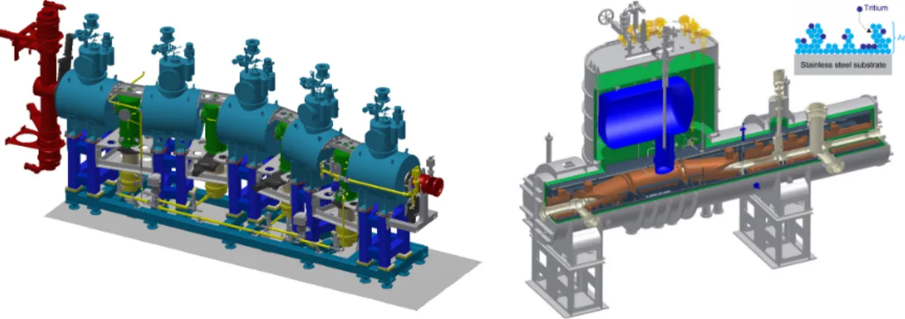
Transport Section

After being created and selected by their angle the β-electrons enter the transport section.

Here they are guided towards the entrance of the spectrometer using magnetic field coils. At the same time the flow of ions and neutral particles is drastically reduced. This is necessary due to the background that would be induced if these particles enter the spectrometer section.

Between the tritium source and the end of the transport section the flow of tritium is reduced by 14 orders of magnitude. This is possible with a combination of a Differential Pumping Section (DPS), where the electrons enter first, and a Cryogenic Pumping Section (CPS), that connects to the spectrometer section. Their experimental setup is shown in fig. 2.5.

Figure 2.5: Illustrations of the two sub systems, that form the transport secion: The Differ- ential Pumping Section (DPS) on the left and the Cryogenic Pumping Section (CPS) on the right. Images taken from [Jan15] (left) and from [Wal13] (right).

To guide the β-electrons the DPS exhibits five superconducting solenoids. Neutral particles are restraint to move in the forward direction by a 20 ^◦ chicanery. This feature improves the pumping efficiency of the four turbomolecular pumps as well. In the DPS a gas-flow reduction by at least five orders of magnitude is achievable. To further prevent the flow of ions a ring electrode as well as electric dipole moments are installed, which will block these particles from moving forward.

At the entrance of the CPS, to complete the ion blocking, an additional ring electrode is

installed. The reduction of the tritium flow by at least another seven orders of magnitude at

the CPS is achieved using a different technique. With the implementation of seven supercon-

ducting magnets the beamline is tilted twice by 15 ^◦ , forcing the remaining neutral particles

to strike the beam tube. The inner surface of this tube is covered by a 3 K argon-frost layer,

which absorbs the neutral particles [Are+18].

2.2 Experimental setup

2.2.2 Spectrometer and detector section

The selection of the electron energies in KATRIN is achieved with two spectrometers that operate with the MAC-E-Filter principle. The first spectrometer, which is called the pre- spectrometer, filters out all the electrons with lower energy. By this, the flux of particles entering the main spectrometer is drastically reduced. This mitigates the background, that is created when the β-electrons hit remaining neutral gas particles in the spectrometer volume.

The precise selection of the electron energy is performed in the main spectrometer. All the electrons that can surpass the retarding potential are collected and counted at the focal plane detector. The two spectrometers and the electron detector are described in the following in more detail.

Pre- and main spectrometer

The pre-spectrometer is located right after the CPS. In operation it rejects all electrons with an energy lower than a few hundred eV below the endpoint. This part of the β-spectrum carries almost no information about the neutrino mass. By applying this energy selection the flux of electrons is reduced, so that only a fraction of 10 ⁻⁶ of the initial particles can pass into the main spectrometer. The chance of exciting neutral residual gas atoms in the large main spectrometer volume is therefore mitigated. For this task of pre-filtering the pre-spectrometer does not require a good energy resolution. Accordingly the size of this component can be rather small.

Electrons that pass the first stage of the energy selection are guided by a 2 m long superconducting transport element towards the main spectrometer. This component of the KATRIN experiment consists of a 23.2 m long stainless-steel vessel with a diameter of 9.8 m.

With this geometric parameters and using the MAC-E-Filter technique an energy resolution of 0.93 eV can be achieved. However, the large size of the vessel makes the main spectrometer vulnerable to the creation of background. To reduce the chance of electrons scattering on molecules in the spectrometer, a high vacuum of 10 ⁻¹¹ mbar is applied. In addition an inner electrode system is installed at the inner surface of the vessel. The electrode system is held on a slightly more negative potential than the spectrometer walls. This rejects low energetic electrons originating from the wall, that fly in the direction of the flux tube.

The electrons that enter the main spectrometer are guided along the magnetic field lines through the volume. In the adiabatically changing magnetic field, that has its lowest value in the analyzing plane, the transverse energy of the electrons is transformed into the parallel direction. Depending on the retarding potential only a fraction of the electrons that entered the spectrometer have enough energy to overcome this threshold. After passing the potential, the electrons are reaccelerated towards the detector, where they are collected and counted [AAB+05; Are+18].

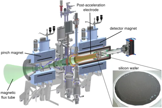
Focal Plane Detector

The focal plane detector of the KATRIN experiment consists of a multi-pixel silicon semicon-

ductor detector with a high energy resolution. The experimental system where it is embedded

can be seen in section 3.3. The electrons exiting the main spectrometer are passing into the

FDP system, where they are guided by a local magnetic field. A post-acceleration electrode

increases the energy of the β-electrons in order to detect them at the FPD in an energy

region, where the background rate from the detector is reduced. With this elevated energy

pinch magnet

detector magnet Post-acceleration

electrode

Figure 2.6: The experimental setup of the Focal Plane Detector. The flux tube is adjusted to the FPD geometry using an additional detector magnet. A post-acceleration elec- trode shifts the electron energy towards higher values. Adapted from [ABB+15;

Wal13].

the electrons from the tritium decay are absorbed at the detector. The sensitiv area of the FPD with a diameter of 90 mm is divided into 148 pixels, where every pixel covers the same area of 44 mm ² . The pixels are arranged into 12 rings, each ring consisting of 12 pixels respectively. In the center of the detector the bulls eye with 4 additional pixels is situated.

This structure allows the study of radial and axial inhomogenities, which could arise due to deviations in the electric or magnetic setup of the experiment.

For the neutrino mass measurement the rate of β-electrons is measured in dependence of the retarding potential, that is set at the main spectrometer. The FPD measures therefore an integral β-spectrum, from which the neutrino mass can be determined [ABB+15].

2.3 Model of the integral β-spectrum

Using the MAC-E-Filter method the KATRIN experiment measures an integral tritium spectrum. To determine the neutrino mass from this data the theoretical and experimental input, that leads to this spectrum, has to be known with high accuracy. The two components that contribute to this spectrum as well as the spectrum itself are addressed in the following.

2.3.1 Differential Decay Spectrum

The theoretical description of the β-decay, that was already addressed in section 1.4.3, has to

be specified to include the properties of the KATRIN tritium source. The usage of molecular

tritium leads to the possible excitation of rotational and vibrational final states in the β-

2.3 Model of the integral β-spectrum

decay. Therefore the energy of the neutrino has to be adjusted by the energy V _f of each final state:

E 0 − E → E 0 − V _f − E = _f (2.4)

Additionally, the decay spectrum has to be summed over each final state f and weighted by the probability that this state occurs. The differential decay spectrum can then be written

as dΓ

dE = C · F(Z, E) · p · (E + m e ) · X

f

·P _f · f · q

² _f − m ² _ν · Θ( f − m ν ). (2.5) Another effect that has to be taken into account is the thermal motion of the tritium molecules. This leads to a broadening of the differential spectrum by the Doppler effect.

It can be addressed by convolving the differential spectrum with a broadening function g:

dΓ dE =

∞

Z

−∞

g(E cms , E _lab ) dΓ

dE (E cms ) dE cms . (2.6)

Here, E _cms is kinetic energy of the electrons in the center-of-mass system and E _lab is the energy in the laboratory frame [KBD+19].

2.3.2 Response function

The second contribution, that has to be known with high precision, is the response function of the experiment. It describes how the β-electrons propagate from the source to the detector.

In KATRIN, the main causes for this response are the energy selection with the MAC-E- Filter and the energy loss of electrons due to scattering in the source.

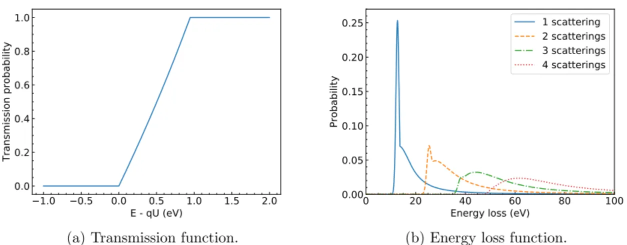
The probability of an electron with energy E to pass the spectrometer with the retarding potential U can be described by the so-called transmission function T (E, qU ) [AAB+05]. For the present isotropic electron source it is given by

T (E, qU ) =



 

 

 

 

 

 

0 E − qU < 0

1−

r

1−

·

A 2 γ+1

1−

r

1−

·

A

0 ≤ E − qU ≤ ∆E

1 E − qU > ∆E

. (2.7)

Here, for the relativistic description of the electrons, the gamma factor γ = _m ^E

e

+ 1 is used.

The relation between the transmission probability and the electron energy is shown in fig. 2.7a for the nominal KATRIN settings.

The energy loss of the electrons traversing the source can be described using an energy loss function f (), that gives the probability of a certain energy loss in a scattering reac- tion, in combination with the function P s (θ) that describes the likelihood that the electron scatters. In the WGTS the electrons can undergo elastic and inelastic scattering processes.

Since only the latter result in a mentionable energy loss, the contribution of elastic scattering is neglected.

The energy loss function is parameterized as f() =



 

 

A ₁ · exp

−2

−

ω

2

< _c A 2 · _ω

^ω

2

+ 4( −

)

≥ c

, (2.8)

1.0 0.5 0.0 0.5 1.0 1.5 2.0 E - qU (eV)

0.0 0.2 0.4 0.6 0.8 1.0

Transmission probability

(a) Transmission function.

0 20 40 60 80 100

Energy loss (eV) 0.00

0.05 0.10 0.15 0.20 0.25

Probability

1 scattering 2 scatterings 3 scatterings 4 scatterings

(b) Energy loss function.

Figure 2.7: Transmission function of the KATRIN experiment for nominal settings and the energy loss function shown for the first four scatterings.

with a Gaussian part describing the losses from excitation processes and a Lorentzian part for the losses originating from the ionization of tritium molecules [KBD+19]. For an electron, that scatters only once, this function returns accurately the energy loss spectrum of this event. In case the electron scatters N-times, the energy loss function has to be convolved (N-1)-times with itself. This is shown in fig. 2.7b on the right for up to four scatterings.

If the electrons exit the source without scattering the energy loss function simply becomes f 0 () = δ().

The probability for the electrons to undergo inelastic scattering depends on the position z in the source, where they were created. This relation can be expressed with an effective column density N _eff , that the electrons see on their way through the WGTS. In addition to the position, N _eff includes the density distribution of ρd as well as the starting angle of the electrons:

N _eff (z, θ) = 1 cos(θ) ·

L/2

Z

z

ρ(z ⁰ ) dz ⁰ . (2.9)

Furthermore, the scattering probability also depends on the inelastic cross section σ _inel [Liu87], that is given by

σ inel (T ) = 4πa ² ₀ T /R

1.5363 ln

4.72 T R

− 0.0097

. (2.10)

It can be seen, that σ _inel depends on the non-relativistic kinetic energy T of the electrons.

The constants a 0 and R are the Bohr radius and the Rydberg energy respectively. Depending on the position and the angle of the electron, the probability to scatter inelastic is determined to be

P _inel,N (z, θ) = (N _eff (z, θ) · σ _inel ) ^N

N ! · exp(−N _eff (z, θ) · σ _inel ). (2.11)

Looking at the case of multiple scattering and taking the mean over the angle and the

2.3 Model of the integral β-spectrum

position z, the probability to scatter N times is then

P N = 1 1 − cos(θ _max )

θ

Z

θ=0

sin(θ)

1

Z

0

P _inel,N (z, θ) dθ. (2.12) The total response function can be retrieved from the transmission function and the functions describing the energy loss. It is given by

R(qU, E ) =

E−qU

Z

0

T (qU, E − )

∞

X

i=0

P N · f N ()d. (2.13)

2.3.3 Integral β-spectrum

Combining the differential decay spectrum with the response function, whose main contribu- tions are the transmission function, the energy loss function and the scattering probability function, leads to the integral β-spectrum

I(qU ) = N ·

E

Z

qU

dΓ

dE (E) · R(qU, E) dE + B (2.14)

with N being a normalization factor and B a background rate of the experiment.

Column density monitoring devices

One of the strengths of the KATRIN experiment is its ability to achieve a high source activity.

Producing and detecting a high number of β-decay electrons is vital to reduce the statistical uncertainty in the neutrino mass measurement. With the ambitious goal of improving the sensitivity on the neutrino mass by one order of magnitude not only statistical but also systematic uncertainties have to be drastically reduced. It is therefore required to monitor the column density of the tritium source with high accuracy.

In this chapter the main experimental parts of KATRIN that can monitor the column density are described. At first, section 3.1 addresses the necessity of monitoring the column density. It is followed by the description of the monitoring devices. Starting in the rear section of the experiment, first the monitoring with the electron gun is outlined in section 3.2.

It is followed by the description of the BIXS detector, which is located in the rear section as well, in section 3.3. A flowmeter sensor in the tritium loop system measures the throughput of the gas and is adressed in section 3.4. Further down the beamline the Forward Beam Monitor (FBM) is able to measure the activity of the tritium source. It is described in detail in section 3.5. The chapter is concluded with section 3.6 where the monitoring of the source activity with the focal plane detector is explained.

3.1 Column density stability

The column density ρd is a major systematic effect in the KATRIN experiment. It determines the amount of gas molecules, that are inside the source. In combination with the tritium purity the column density gives the activity of the WGTS. The product of ρd with the cross section σ determines the scattering probability of the β-electons in the source.

A precise knowledge of the absolute value and the variation over time is crucial for the KATRIN analysis. The absolute value has to be known to determine the scattering probabilities of the electrons with great precision. Since the KATRIN experiment measures an integral β-spectrum, variations of the column density during a tritium scan can bias the analysis of the tritium data. To mitigate these effects the KATRIN experiment features different monitoring devices, that can measure the absolute value of the column density as well as observe fluctuations on small time scales.

3.2 Photo-electron source

One of the tasks of the photo-electron source, a calibration device that was developed to

provide a mono-energetic and angular-selective electron beam, is to determine the column

density with a precision of 0.2 % [AAB+05].

3.2 Photo-electron source

Figure 3.1: Illustration of the production of electrons with the photoelectric effect (left). A fiber guides UV light towards a photocathode, which consists of a thin metallic coating. Illuminated from behind the metal surface emits electrons with defined energy.

The setup of the electron gun (right). The grounded cage contains the accelera- tion setup, which is described in figure fig. 3.2, and is installed in a gimbal mount allowing the movement around two axes. A vacuum flange sealing the device in the rear section contains the feed-throughs needed for the optical fibers, HV and movement control. Taken from [Zac14] and [Beh16].

Situated in the rear section of the experiment, it emits electrons from a metal surface via the photoelectric effect as depicted in figure fig. 3.1 (left). The experimental setup is given in figure fig. 3.1 (right). Photons, produced by a light source, with a well defined wavelength are guided to a photocathode using optical fibers. There they create electrons with an energy E depending on the photon frequency and the work function of the cathode:

E = hν − Φ > 0. (3.1)

To reach their nominal energy E 0 , which is set to be close to the tritium endpoint the electrons are accelerated against the ground electrodes at the spectrometer entrance.

Electrons that are emitted from a flat photocathode exhibit angles that follow a cos θ- distribution [PB02]. By applying a non-adiabatic acceleration electrons with a well-defined angle can be produced. For this, the electron source features a setup as depicted in figure fig. 3.2. The potential difference between the back plate and the front plate U _acc = U _front − U _back creates a strong homogeneous electric field. Tilting the whole setup by a defined angle with respect to the magnetic field lines causes a strong non-adiabatic acceleration of the electrons narrowing their the angular distribution. This technique allows the calibration of a variety of experimental properties, for which distinct angular settings are needed [Beh16; Zac14].

To produce the electron beam the e-gun can be operated using two different light sources:

a pulsed laser that produces monochromatic UV light with a wavelength of 266 nm, and a

laser-driven light source (LDLS), which can create photons with a variable wavelength from

about 240 nm to 320 nm. To monitor the light intensity a beam splitter in combination with

a photodiode is used.

Figure 3.2: Schematic overview of the electron source setup. Created via the photo-effect from a photocathode on the back plate the electrons are accelerated in a strong electric field created by the potential difference between front plate and back plate. The grounded cage, that is shielding the potentials from outside influences, can be rotated around P e resulting in a tilt angle α _P against the direction of the magnetic field. Figure taken from [Zac14].

For the determination of the column density with the electron gun the electrons are sent through the WGTS towards the focal plane detector and the count rate is measured at different surplus energies δE = E − qU . The obtained data is fitted to a model response function and the absolute value of the column density can be extracted as a result of the fit with high precision. This method was implemented in the frame of this thesis and is explained in more detail in chapter chapter 4.

Since this determination of ρd with the e-gun can not be conducted at the same time as the measurement of the tritium spectrum it should be applied in order to maximize the time available for the measurement of the neutrino signal. In this work a study with Monte Carlo (MC) data to reduce the time needed for a precise determination of the column density with the electron gun is given in chapter chapter 6.

3.3 Beta Induced X-ray Spectrometry

The activity of the WGTS can be monitored with the technique of the Beta Induced X-ray Spectrometry (BIXS) [MWH98]. The underlying principle is the detection of bremsstrahlung X-rays, that are produced by the β-electrons from the tritium decay. The intensity of the measured photons can be translated into the tritium activity of the WGTS.

In KATRIN two BIXS detectors are located in the rear section of the experiment as

shown in fig. 3.3. They are positioned in a way to monitor the intensity of X-rays created at

the rear wall surface. Almost all of the β-electrons reach the rear wall either directly or by

being reflected back due to the filtering principle of the pre- and main spectrometer. This

high flux of β-electrons creates intense X-Ray radiation which can be monitored by the BIXS

detectors. To shield the silicon drift detectors (SDD), which detect the photon signals, from

the tritium gas of the WGTS, two transparent gold-coated beryllium windows are positioned

3.4 Tritium loop sensor

in front of the them. The coating of the windows with gold helps to reduce the detection of X-rays which are not produced at the rear wall but are created by absorbed tritium.

rear wall

SDD X-ray detector

X-ray detector electronics Au coated

Be window

Figure 3.3: Overview of the main BIXS related experimental components. Electrons created via β-decay in the WGTS reach the rear wall and produce X-rays. These photons are detected by two silicon drift detectors, which are protected from tritium contamination by transparent gold-coated beryllium windows. Adapted from [R¨ ol15].

To monitor the column density of the tritium source with the BIXS detectors in addition to the precise determination of the activity also the tritium purity has to be known accurately.

The amount of produced X-ray radiation relates to the active part of the source gas. To monitor the absolute amount of gas molecules in the WGTS the measured activity has to be corrected with the value of the tritium purity which is measured separately via laser Raman spectroscopy (LARA). Further it is important to mitigate contaminations of the rear wall and beryllium window surface, since these would affect the amount of X-rays detected and therefore influence the measurement of the activity.

Using the BIXS detectors an accurate monitoring of the relative change of the column density is possible. Due to the observation of an intense X-ray signal the fluctuation of the activity can be determined with high precision on a short timescale. However, a precise measurement of the absolute value of ρd is not possible and is also not the intention of the Beta Induced X-ray Spectrometry [R¨ ol15].

3.4 Tritium loop sensor

As explained in section 2.2.1, the tritium gas of the WGTS is circling in a closed loop system

to create a stable column density in the source. A variety of dedicated sensors is measuring

constantly parameters like the pressure, temperature and gas flow in this complex system.

By observing the relative change of the values of these parameters the column density can be monitored accurately.

One sensor that is located close to the inlet of the tritium gas into the WGTS measures the flow of the gas through the pipe ^dV _dt . Combining it with the value for the buffer vessel pressure P _buffer allows the determination of the throughput q:

q = dV

dt · P _buffer (3.2)

The column density of the tritium source can then be estimated using gas flow simulations based on the throughput value input. This allows the determination of the absolute value of ρd with a precision of ≈ 2 % [Kuc16]. In Addition the observation of the throughput with the flow meter allows the monitoring of the column density stability during tritium measurements with good accuracy.

3.5 Forward Beam Monitor

Similar to the BIXS detector the Forward Beam Monitor (FBM) can measure the activity of the tritium source. It is situated at the end of the transport section, shortly before the β-electrons enter the pre-spectrometer. With the experimental setup, as shown in fig. 3.4, it can be inserted directly into the flux tube of the beamline. Being movable radially as well as linear in the x-direction it can be positioned over the whole flux tube area. The silicon p-i-n diodes have an energy resolution of σ _FWHM ≈ 2 keV.

Figure 3.4: Schematic overview of the experimental setup of the FBM. The silicon detector consisting of two p-i-n diodes is sitting on a detector board, that is in addition equipped with a hall sensor and a temperature gauge. A 2 m long bellow enables the positioning in the flux tube. The standard monitoring position is at the outer rim of the flux tube [Are+18].

During tritium decay measurements the FBM can monitor the β-electron flux with high precision due to the large number of electrons being detected. To maximize the statistics the energy threshold can be lowered to allow also the detection of low energetic electrons.

In addition to the count rate, the FBM also measures the β-spectra, allowing further study of these data.

To monitor the column density the activity, that the FBM measures, has to be corrected

by the tritium purity. It is then possible to precisely determine relative fluctuations of ρd.

3.6 Focal Plane Detector

The absolute measurement with high precision is similar to the case of the BIXS detector not feasible.

3.6 Focal Plane Detector

The activity of the tritium source is also imprinted in the β-spectrum that is measured with the FPD. Measurement points deep in the spectrum provide a strong signal that is sensitive to activity fluctuations of the WGTS.

To accurately monitor the column density with this method corrections have to be ap- plied to the measured electron rate. One of these corrections arises due to the uncertainty of the high voltage setting. When comparing the electron rates at a certain retarding poten- tial, deviations in the rate can arise due to slightly different voltage settings. The measured electron rate therefore has to be adjusted to the underlying voltage value. Since the FPD measures the electrons that traverse both spectrometers the ability to overcome the retarding potentials depends on the energy loss in the WGTS. For higher column densities, assuming the tritium purity stays constant, the activity in the source is larger resulting in a higher electron rate measured at the FPD. At the same time the probability to undergo inelastic scattering in the source is increased reducing the chance of electrons to overcome the re- tarding potential. Hence, a correction is applied that counters this effect. As in the other activity measurements the data has to be corrected by the tritium purity to be sensitive to the whole amount of gas in the WGTS.

By monitoring the electron rate that is measured deep in the β-spectrum and applying the necessary corrections one is able to determine column density fluctuations with the FPD.

The uncertainty of this measurement depends on the total number of detected electrons as well as the uncertainties of the underlying corrections. In addition spending time at a measurement point far away from the expected neutrino signal reduces the available time for the neutrino mass measurement. Fluctuations of the column density can therefore be observed only on the time scale of hours.

Another possibility to obtain the column density, which was investigated in this thesis,

is from the tritium spectrum itself. Here the column density is treated as a free parameter

in the spectral fit. More details are given in section 7.1.

Determination of ρdσ with the photo-electron source

The goal to measure the neutrino mass with a sensitivity of 200 meV with the KATRIN experiment requires a precise knowledge of the response function of the experiment. This function describes the propagation of the β-electrons from the source to the detector. An important component of the response function is the description of the energy loss of the electrons due to inelastic scattering on the gas molecules in the source. The probability for an electron to scatter in this way depends on the column density of the source ρd and the inelastic scattering cross section of the electrons σ _inel . Hence, a precise knowledge of ρdσ is necessary to obtain an accurate description of the response function and therefore limit the systematic uncertainty of the neutrino mass measurement. To achieve the goal of the KATRIN experiment to measure the neutrino mass with a sensitivity of 200 meV requires ρdσ to be known with a precision of 0.2 % [AAB+05].

A determination of the column density and the inelastic cross section can be achieved with dedicated measurements using the photo-electron source. A mono-energetic electron beam with a high and stable rate is created in the rear section of the experiment and guided through the beamline towards the detector. Traversing the source, the electrons can undergo inelastic scattering and in the process lose energy. Only the electrons, that still have enough energy to pass the spectrometers are observed at the detector. Measuring the electron rate at different retarding potentials and fitting the model of the response function with ρdσ as a free parameter to this data allows an accurate determination of ρdσ.

This chapter describes in detail the necessary components to retrieve the column density and the inelastic scattering cross section from a measurement with the electron gun. It is structured in the following way: Section 4.1 describes the response model of the electrons created with the e-gun. The measurement principle to determine the column density with these photo-electrons is addressed in section 4.2. A brief overview of the software framework, that is used in the analysis, is given in section 4.3. The chapter is concluded with section 4.4, in which the determination of ρdσ with a response fit is explained and the results of the ρdσ determination for the first neutrino mass measurement are shown.

4.1 Response model

The electrons created with the e-gun differ from the β-electrons of the tritium decay in regard

to the starting position, the energy and the angular distribution. Since they are used in a

variety of calibration measurements, that cover different parts of the experimental setup,

they are produced at a fixed position in the rear section of the experiment, as explained

in section 2.2.1. A narrow energy distribution of the electrons as well as the ability to

4.1 Response model

produce them with a specific pitch angle θ is mainly required to investigate the transmission properties of the spectrometer. A precise description of the response function for the photo- electrons is necessary to infer the column density from the measured data. It has to include the properties of the e-gun electrons, that differ from the properties of the β-electrons, whose model was described in section 2.3.

4.1.1 Transmission function

The electrons created in the electron gun start in the rear section of the experiment and are guided magnetically towards the detector. Similar to the β-electrons they can only surpass the main spectrometer, if they possess more energy in the longitudinal direction than is required to overcome the retarding potential.

In the case of an ideal electron source, that produces mono-energetic electrons with pitch angles of 0 ^◦ , the transmission function can be described as a step function. All the electrons with a positive surplus energy E − qU in the analyzing plane are able to traverse the spectrometer and can travel towards the FPD.

The actual photo-electron source of the KATRIN experiment produces electrons with a narrow energy and angular distribution and can be adjusted to emit electrons with a certain pitch angle θ. The transmission function has to take these properties into account and can be described by

T(E, qU ) =

∞

Z

E−qU

η(E _e )

θ

Z

0

ξ(θ) dθdE _e . (4.1)

Including the integration over the energy and the angular distribution the function now accurately describes transmission of the electrons [Beh16].

4.1.2 Energy distribution

The e-gun uses the photoelectric effect to create the electrons by illumination with UV light with a frequency ν onto a metal surface. The energy of the created electrons is hence

E = hν − Φ > 0, (4.2)

where Φ is the work function of the metal surface. Because the electrons, that are situated in the metal, exhibit an energy distribution according to the properties of the photocathode material, the frequency of the illuminating light can be used to narrow the energy distribution of the emitted electrons, by tuning it to match the work function.

A simple theoretical expression of the emission of electrons via the photoelectric effect

was given more than 50 years ago by Berglund and Spicer [BS64a; BS64b] and is based

upon the work of Fowler, who studied the dependency of the photoelectric current on metal

temperatures [Fow31]. The simplified model explains the photoemission in three steps: the

excitation of the electron in the photocathode material, the transportation towards the

surface and the emission into the vacuum. Starting at the beginning of the three step

process and assuming a metallic photocathode, the electron resides in the conduction band

and is excited by a photon with a frequency in the ultraviolet region. The energy of the

excited electron depends on the photon energy as well as on the band structure of the cathode

material. On the way towards the surface the electron has a large probability to scatter with