Analysis of longitudinal variations in North Paci fi c alkalinity to improve predictive algorithms

Analysis of longitudinal variations in North Paci fi c alkalinity to improve predictive algorithms

Claudia H. Fry¹, Toby Tyrrell¹, and Eric P. Achterberg^1,2

1National Oceanography Centre Southampton, University of Southampton, Southampton, UK,²GEOMAR Helmholtz Centre for Ocean Research, Kiel, Germany

Abstract

The causes of natural variation in alkalinity in the North Pacific surface ocean need to be investigated to understand the carbon cycle and to improve predictive algorithms. We used GLODAPv2 to test hypotheses on the causes of three longitudinal phenomena in Alk*, a tracer of calcium carbonate cycling.

These phenomena are (a) an increase from east to west between 45°N and 55°N, (b) an increase from west to east between 25°N and 40°N, and (c) a minor increase from west to east in the equatorial upwelling region. Between 45°N and 55°N, Alk* is higher on the western than on the eastern side, and this is associated with denser isopycnals with higher Alk* lying at shallower depths. Between 25°N and 40°N, upwelling along the North American continental shelf causes higher Alk* in the east. Along the equator, a strong east-west trend was not observed, even though the upwelling on the eastern side of the basin is more intense, because the water brought to the surface is not high in Alk*. We created two algorithms to predict alkalinity, one for the entire Pacific Ocean north of 30°S and one for the eastern margin. The Pacific Ocean algorithm is more accurate than the commonly used algorithm published by Lee et al. (2006), of similar accuracy to the best previously published algorithm by Sasse et al. (2013), and is less biased with longitude than other algorithms in the subpolar North Pacific. Our eastern margin algorithm is more accurate than previously published algorithms.

1. Introduction

Total alkalinity, hereafter referred to as alkalinity, is typically determined as part of seawater carbonate chem- istry observations. Alkalinity is the excess of proton acceptors over proton donors [Wolf-Gladrow et al., 2007].

It is one of four measurable carbonate chemistry variables, with the others being dissolved inorganic carbon, pH, and the partial pressure of carbon dioxide (pCO₂). We can calculate the entire carbonate system with any two of these variables, along with temperature, pressure, salinity, phosphate, and silicate concentrations.

Alkalinity is useful because it behaves in a conservative manner when water masses mix and is independent of changes in temperature and pressure, unlikepCO₂and pH [Dyrssen and Sillén, 1967;Wolf-Gladrow et al., 2007]. This allows us to develop linear relationships to predict alkalinity from common hydrographic mea- surements, like temperature and salinity. These relationships can then be used to constrain the carbonate system from standard measurements when a carbonate variable is unavailable. This approach is more diffi- cult forpCO₂and pH due to their nonlinear relationship with temperature and salinity.

The main causes of variation in surface ocean alkalinity are dilution and concentration as a result of precipita- tion, evaporation, river discharge, and sea ice formation and melt [Millero et al., 1998;Friis et al., 2003;Cai et al., 2010]. Since these processes also strongly influence ocean salinity, alkalinity is often considered a function of salinity due to its strongly conservative nature [e.g.,Chen and Millero, 1979;Millero et al., 1998;Lee et al., 2006;

Land et al., 2015]. However, alkalinity is also affected by nonconservative processes, for example, biological organic matter production and calcification [Brewer and Goldman, 1976;Wolf-Gladrow et al., 2007;Kwon et al., 2009]. It is therefore important to determine the causes of local nonconservative deviations in alkalinity (variations from the relationship with salinity) to improve our understanding of the controls on ocean carbo- nate chemistry and its role in climate change and ocean acidification.

The North Pacific, from the equator to the Bering Sea, is a region of the global ocean where the controls on alkalinity are not yet well understood.Chen and Pytkowicz[1979]first identified a longitudinal gradient in salinity-normalized alkalinity in the subpolar North Pacific and in this area; unlike in other regions,Lee et al.

[2006] could not model the distribution of surface ocean alkalinity using salinity and temperature alone and used longitude as an additional predictor variable. The results matched the observed alkalinity variations, but the approach was no longer mechanistic.

Global Biogeochemical Cycles

RESEARCH ARTICLE

10.1002/2016GB005398

Key Points:

•Longitudinal variations in alkalinity in the North Pacific are influenced by physical processes

•Predictive algorithms for alkalinity are improved by using indicators of physical processes

Correspondence to:

C.H. Fry,

claudia.fry@noc.soton.ac.uk

Citation:

Fry, C. H., T. Tyrrell, and E. P. Achterberg (2016), Analysis of longitudinal varia- tions in North Pacific alkalinity to improve predictive algorithms,Global Biogeochem. Cycles,30, 1493–1508, doi:10.1002/2016GB005398.

Received 17 FEB 2016 Accepted 25 SEP 2016

Accepted article online 28 SEP 2016 Published online 15 OCT 2016

©2016. American Geophysical Union.

All Rights Reserved.

Sasse et al.[2013] improved onLee et al.[2006] by using more predictor variables (temperature, salinity, dis- solved oxygen, silicate, and phosphate), while dividing the ocean into the same regions asLee et al.[2006].

They compared the results of their multiple linear regression with a Self-Organizing Multiple Linear Output (SOMLO); however, this did not improve the prediction of alkalinity in the North Pacific. The accuracy of the SOMLO was only 2.7% greater in the North Pacific (temperature<20°C; salinity between 31 and 35) and was 2.1% less accurate in the equatorial Pacific. They commented that there are few nonlinearities in the carbonate system; therefore, using a nonlinear model does not provide an improvement. Henceforth, we only refer to the multiple linear regression bySasse et al.[2013].

In the tropical ocean, bothMillero et al.[1998] andLee et al.[2006] noted that the eastern equatorial upwelling region had a higher salinity-normalized alkalinity than the rest of the tropical oceans.Fry et al.[2015] andIshii et al.[2004], on the other hand, did not observe any longitudinal variation in salinity-normalized alkalinity in these ocean regions. However, it is possible that a different relationship from the rest of the tropical region is still required. Some of the predictor variables may be affected by the equatorial upwelling, and although alka- linity is not, the relationship between alkalinity and the predictor variables is changed by the upwelling. For example, if upwelling waters are colder than nonupwelling waters but do not contain elevated Alk* values (see below for Alk* definition), then the relationship with the predictor (temperature) may change and a new equation is necessary even though Alk* values are not different from those outside the upwelling region.

The study of the factors controlling variability of the oceanic carbonate system is important because of its central role in climate change and ocean acidification. There is, however, a limited amount of alkalinity data compared to other hydrographic measurements such as temperature, salinity, and nutrients (GLODAPv2 has about 42,000 casts, whereas the World Ocean Database contains over 3,000,000 casts). As a result of the insuf- ficient temporal and spatial coverage of the global ocean, algorithms are employed to predict alkalinity values using commonly measured variables such as temperature and salinity. These algorithms therefore provide greater alkalinity coverage of the ocean and are also of importance for verification of biogeochemical models as it is difficult to model alkalinityfields with a high level of accuracy.

We have recently introduced Alk* (equation (1)) as a tracer of calcification, dissolution of calcium carbonate, and the movement of the dissolution products via physical circulation [Fry et al., 2015]. Alk* illuminates these processes as it removes other common controlling factors of variation, namely, evaporation and precipita- tion, river inputs, and biological uptake and release of ions.

Alk*¼Alk_mþ1:36NitAlk_r

Sal 35þAlk_r2300 (1)

where Alk_mis the measured alkalinity (μmol kg¹), Nit is the nitrate concentration (μmol kg¹), Alk_ris the identified river alkalinity (μmol kg¹) in ocean areas affected by river inputs, and Sal is the salinity.

The aim of our work is to determine the factors controlling alkalinity in the surface waters of the North Pacific Ocean. We test a series of hypotheses that explore longitudinal variations in Alk* in the zonal bands 45°N–55°

N, 25°N–40°N, and 15°S–10°N. We then derive two algorithms that predict alkalinity in surface waters, for both the entire Pacific Ocean north of 30°S and also in the eastern margin of the North Pacific. Each algorithm con- sists of three equations and the relevant definitions of how to choose which equation to use for each location.

2. Hypotheses

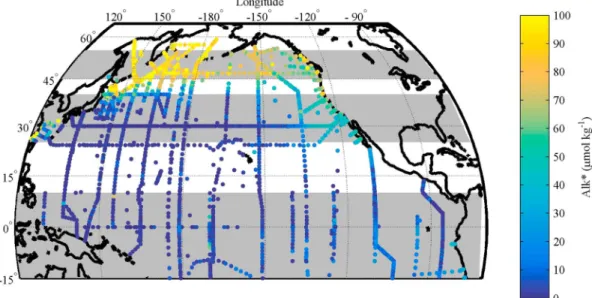
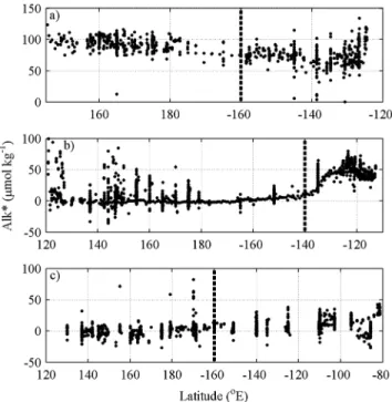
The Alk* distribution in the surface waters of the North Pacific shows distinct longitudinal gradients at differ- ent latitudes (Figure 1): (1) between 45°N and 55°N, Alk* is higher in the west than the east (Figure 2a); (2) between 25°N and 40°N, Alk* at the eastern edge of the Pacific is higher than further west (Figure 2b); and (3) in the eastern equatorial Pacific there is only a minor increase in Alk* despite a pronounced reported increase in salinity-normalized alkalinity [Millero et al., 1998;Lee et al., 2006] (Figure 2c). The differences between east and west in all three latitudinal bands are significant (Table 1). The divide is situated further east for the 30°N zonal band as we are looking to explain a localized feature and a more central divide would bias thet test results. We developed a series of hypotheses for each of the phenomena (the gradients just described) and tested the hypotheses using observational data. For all three latitudinal bands, we considered the alternative possibility of the patterns being caused by errors in data such as a bias of one cruise or random error in a few data points.

Phenomenon 1: Between 45°N and 55°N, Alk* is higher in the northwest Pacific than in the northeast Pacific.

Hypothesis 1.1. Winter mixing yields higher Alk* values to the west, as it reaches greater depths than on the eastern side.

Hypothesis 1.2. Denser isopycnals with older water containing elevated Alk* are closer to the surface on the western side.

Hypothesis 1.3. Anaerobic processes in shelf sediments (which enhance Alk*) exert a stronger influence on the western side.

Phenomenon 2: Between 25°N and 40°N, Alk* is higher toward the eastern edge of the Pacific than further west.

Hypothesis 2.1. Previously unidentified outflow from North American rivers affects Alk*.

Hypothesis 2.2. Upwelling increases Alk* along the North American coast.

Hypothesis 2.3. High Alk* waters are transported southward from the northeast Pacific by the California Current, but this process does not occur in the northwest Pacific, where the northwardflowing Kuroshio Current dominates.

Phenomenon 3: In the equatorial Pacific region, there is little increase in Alk* from the west to the east.

Hypothesis 3.1. In the majority of phases of the El Niño–Southern Oscillation (ENSO) there is limited upwelling of Alk*.

Hypothesis 3.2. The upwelled waters do not come from a sufficiently great depth to contain enhanced Alk*.

Figure 1.Alk* in the surface waters (<30 m) of the North Pacific using data from the GLODAPv2 database. No rivers were included in the calculation of the Alk* values. The three areas shaded in grey indicate the areas of the three phenomena investigated in this study.

Hypothesis 3.3. High Alk* waters are upwelled, but calcification and export rapidly remove Alk* from the sur- face ocean.

3. Methodology

Alkalinity and other variables were obtained from the GLODAPv2 database [Olsen et al., 2016]. Data from depths of less than 30 m were defined as being from the surface mixed layer. Alk* was calculated using equa- tion (1), and no correction for riverine alkalinity inputs was applied because no substantial areas influenced by rivers have previously been identified in the North Pacific [Fry et al., 2015]. Shelf areas are included in our approach, which is different to our previous study [Fry et al., 2015]. The typical accuracy of alkalinity mea- surements is 3μmol kg¹[Dickson et al., 2003] and 3.02μmol kg¹for Alk* [Fry et al., 2015]. Annual mean dis- solved oxygen and nitrate gridded to 1° were obtained from the World Ocean Atlas 2013 [Garcia et al., 2014a, 2014b]. Mixed layer depth data were obtained from the National Oceanic and Atmospheric Administration (NOAA) [Monterey and Levitus, 1997]. The mixed layer depth data were gridded to 0.5° for each month, and mixed layer depth was defined using a variable potential density criterion corresponding to a change in tem- perature of 0.5°C [Monterey and Levitus, 1997]. The maximum mixed layer depth used was the largest of the monthly values for each grid point. The resulting maximum mixed layer depths occurred in the northern hemisphere winter, with February the most common month for the deepest mixed layer. The effect and Figure 2.Longitudinal variations in Alk* along the three longitudinal bands presented in Figure 1: (a) 45°N to 55°N, (b) 25°N to 40°N, and (c) 15°S to 10°N. The dashed lines represent the longitudinal divide between east and west. For phenomenon 1 (Figure 2a) and 3 (Figure 2c), 160°W was used because is it approximately central in the basin. Phenomenon 2 (Figure 2b) is a local feature so 140°W was used to separate data in the local area from the rest of the basin.

Table 1. Alk* Difference from East to West in the North Pacific Band

Longitudinal Divide

Between East and West p^a Degrees of Freedom tStatistics^b Mean in West (μmol kg¹) Mean in East (μmol kg¹)

45°N–55°N 160°W <0.001 931 23.6 95.3 72.2

25°N–40°N 140°W <0.001 1602 24.1 9.5 46.9

15°S–10°N 160°W <0.001 1619 20.0 0.8 10.7

aProbability with the null hypothesis for each band is that the means of both boxes are equal.

bTwo-sample, two-tailedttest.

strength of the ENSO were tested using a Multivariate ENSO Index from NOAA [http://www.esrl.noaa.gov/

psd/enso/mei/]. The index is produced monthly and calculated using the current and previous month.

Unless otherwise stated, the areas analyzed are 45°N to 55°N for phenomenon 1, 25°N to 40°N for phenom- enon 2, and 15°S to 10°N for phenomenon 3. The chosen area for phenomenon 3 (equatorial region) is asym- metrical across the equator because the peak in nitrate occurs south of the equator in the Pacific Ocean [Garcia et al., 2014b] as a result of geographic asymmetry [Xie and Philander, 1994].

4. Results and Discussion

4.1. Alk* Variations Along Approximately 50°N in the North Pacific

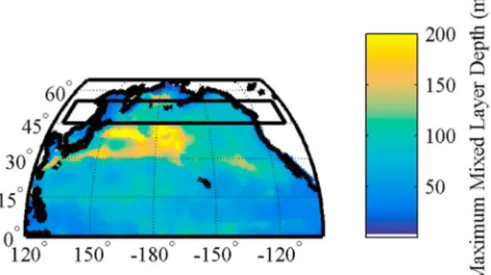
The maximum mixed layer depths at 40°N are greater in the west than the east (Figure 3). However, the area of interest (the black box) is to the north of the region of the greatest maximum mixed layer depths. The rela- tionship between maximum mixed layer depth and the surface Alk* is weak (R²= 0.0578,N= 3889) (Figure 4).

Therefore, surface Alk* appears to be unrelated to the maximum mixed layer depth (refuting hypothesis 1.1).

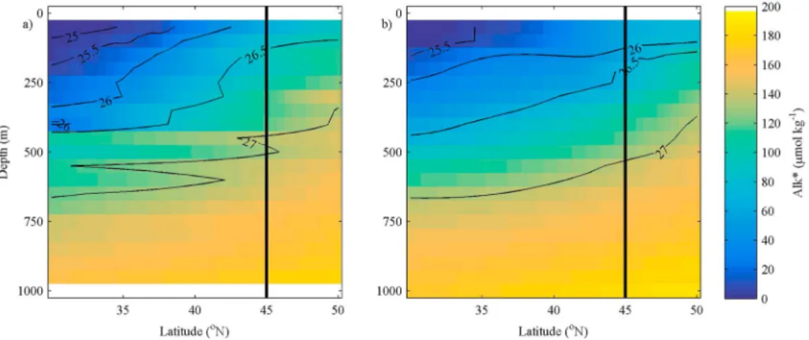
Alk* appears to follow the lines of potential density, with denser waters containing higher Alk* occurring closer to the surface in the west than in the east (right side of Figure 5a compared to right side of Figure 5b). The depths of isopycnals and Alk* concentrations in the west and the east are presented in Table 2. These show that the mean depth of isopycnals is shallower in the west than the east of the North Pacific, and this is matched by shallower mean depths of Alk* concentrations in the west than in the east. Further, the Pearson’srcorrelation coefficient between potential density and Alk* is 0.890 in the region of phenomenon 1, which shows that there Figure 3.Maximum mixed layer depths in the North Pacific Ocean. The black box marks the area defined as phenomenon 1.

Figure 4.Alk* in surface waters of the North Pacific between 45°N and 55°N as a function of maximum mixed layer depth.

is a strong positive correlation. These observations confirm hypothesis 1.2; Alk* in the surface ocean is affected by entrainment of waters from dense isopycnal layers.

Sulfate uptake affects alkalinity by changing the charge balance of seawater. This causes alkalinity to increase in order to counteract the change [Wolf-Gladrow et al., 2007]. Sulfate reduction is an anaerobic process; there- fore, if this process contributes to phenomenon 1 (hypothesis 1.3), we would also expect lower dissolved oxy- gen concentrations in the western region of the North Pacific zonal band compared with the eastern region.

However, anoxia is not prevalent in surface waters due to rapid exchange processes of oxygen with the atmo- sphere. Using the World Ocean Atlas, the dissolved oxygen concentrations in the surface waters in the west are higher (mean = 7.1 mL L¹, standard deviation = 0.4 mL L¹) than in the east (mean = 6.5 mL L¹, standard deviation = 0.6 mL L¹). The east and west North Pacific between 45°N and 55°N have different oxygen con- centrations at all depths (two-samplettests;p<0.001). However, the difference at 100 m is opposite to what is required for hypotheses 1.3 to be accepted (oxygen is higher in the west than the east). There is a band of low oxygen concentrations along the Aleutian Arc at about 200 m, a region where sulfate reduction in sedi- ments has been observed [Hein et al., 1979;Elvert et al., 2000]. However, the Aleutian Arc is not where the highest Alk* is observed and the area seems to have decreased oxygen levels (<2 mL L¹) only below 200 m.

The east-west Alk* gradient occurs in measurements from many cruises. The gradient is therefore unlikely to be an artifact caused by measurement error on any single cruise. However, all Japanese cruises in GLODAPv2 had a systematic adjustment applied to their alkalinity data of +6μmol kg¹. This was done in order to make the deepwater values of the Japanese cruises consistent with data from other countries at crossover stations.

If this adjustment was incorrect then it could have created the observed east-west trend, as the Japanese cruises took place mainly in the western North Pacific. To test this possibility, we subtracted 6μmol kg¹from all the Japanese alkalinity data, reversing the adjustment in GLODAPv2. This reduced the mean Alk* value in the west from 95.8 (Table 1) to 89.9μmol kg¹ and the mean Alk* value in the east from 72.2 to 71.0μmol kg¹. Therefore, a significant east-west gradient remained, showing that the adjustment in GLODAPv2 was not the cause of the east-west trend.

Our data suggest that the alkalinity variation in the surface waters of the North Pacific, between 45°N and 55°N, is caused by denser isopycnals with higher Alk* occurring at shallower depths on the western side than on Figure 5.Meridional sections of Alk* (μmol kg¹; color) and potential density (σθ; contours) at (a) 165°E (WOCE cruise P13N in 1992) and (b) 135°W (WOCE cruise P16N in 2006) obtained from GLODAPv2. The vertical black line represents the southern edge of the area of phenomenon 1.

Table 2. Mean Depths (m) of Differentσθand Alk* Values^ain the East Compared with the West for the Latitudinal Region Between 45°N and 55°N

Mean Depth at Whichσθ= 26 Mean Depth at Whichσθ= 27 Mean Depth at Which Alk* = 100 Mean Depth at Which Alk* = 150

West of 160°W 28 328 46 399

East of 160°W 101 412 172 528

aData were interpolated using a smoothing spline, where the smoothing parameter isp= 0.5.

the eastern side (hypothesis 1.2). This east-west difference is likely driven by Ekman pumping, which brings deeper water closer to the surface on the western side [Talley, 1985, 1988].

4.2. Alk* Variations Along About 30°N in the North Pacific

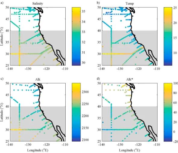
Between 25°N and 40°N, Alk* concentrations are higher in the eastern coastal region than in the open ocean (Figure 6). Along the coast at about 45°N, the Alk* is elevated (approximately 80μmol kg¹) and the salinity and alkalinity are low (about 32 and 2180μmol kg¹, respectively), suggesting that this enhanced Alk* is caused by unaccounted for riverine inputs. But in the area of interest along the coast (25–40°N), the salinity and alkalinity are both higher than the average of all the data between 25 and 50°N (33.5 versus a mean of 32.7 and 2244μmol kg¹versus a mean of 2216μmol kg¹) and the temperature is lower than offshore (14.3°C versus 17.9°C offshore). This indicates that the enhanced Alk* is caused by upwelling.

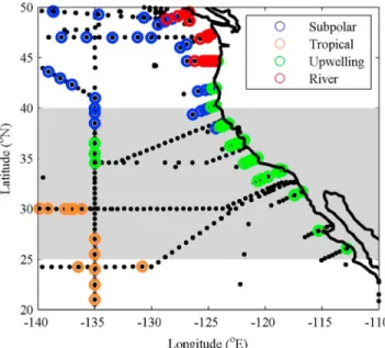
We partitioned the eastern data into four groups to represent subpolar, tropical, upwelling, and river- influenced waters (Table 3 and Figure 7). The properties of offshore subpolar and tropical water were derived Figure 6.The distribution of (a) salinity, (b) temperature (°C), (c) alkalinity (μmol kg¹), and (d) Alk* (μmol kg¹) in the sur- face waters of the North Pacific Ocean close to the North American continent. The grey shaded area represents the area of phenomenon 2.

Table 3. The Criteria for Delineation of Surface Waters

Area Salinity Alkalinity (μmol kg¹) Alk* (μmol kg¹)

Subpolar 32.5 ± 0.2 2184 ± 18 68 ± 17

Tropical 35.0 ± 0.3 2304 ± 23 9 ± 9

Upwelling >33 >50

River <32 <2170

by using data within regional boxes and calculating the mean and standard deviations. These boxes were defined as between 45°N and 55°N and 130°W and 150°W for the subpolar box and between 15°N and 25°N and 120°W and 150°W for the tropical box. Water wasflagged as subpolar or tropical influenced if its salinity, alkalinity, and Alk* were all within 1 standard deviation of the mean of the defined box.

Figure 7 shows that the groups are distributed in geographical clusters according to where each set of forcing factors had the strongest influence. For example, river-influenced points are situated in the coastal region.

This provides evidence that all three factors enhance Alk* in different areas. Away from the coast, a small amount of mixing between subpolar water and tropical gyre waters takes place (hypothesis 2.3). In the coastal region, upwelling increases Alk* in the south (25–42°N) and river inputs increases Alk* in the north (42–50°N; Figure 7). However, the river-influenced waters are to the north of the area we have highlighted as anomalous, hence ruling out hypothesis 2.1 for the latitudinal region under investigation.

Phenomenon 2 is unlikely to be due to random error because it is derived from a large and coherent data set from a range of cruises. The different surface waters identified in this data set also agree with those reported byJiang et al.[2014]: low-temperature, high-salinity water upwelling off the tropical coast and water from the Columbia and Fraser Rivers (both with alkalinities of about 1000μmol kg¹[Park et al., 1969;Dahm et al., 1981; Amiotte Suchet et al., 2003; de Mora, 2008]), influencing regions near the coastline further north.

Jiang et al.[2014] also reported lower salinities (<32.5) in the California Current than in the open ocean (>32.5), which is in agreement with our definitions of subpolar and tropical waters (Table 3).

Figures 1 and 2 show a few anomalously high Alk* values adjacent to the East China Sea at 30°N (21 points with an Alk* greater than 100μmol kg¹), although the average is not much different from elsewhere, unlike toward the eastern side. Alk* in the East China Sea is likely to be influenced by the river alkalinity inputs from the Yangtze and Yellow Rivers [Chen, 1996;Tsunogai et al., 1997;Kang et al., 2013] and sulfate reduction due to eutrophication [Chen and Wang, 1999;Chen, 2002;Lin et al., 2002;Cai et al., 2011].

In conclusion, wefind that Alk* is enhanced in the eastern North Pacific around 30°N through upwelling of dee- per waters with enhanced dissolved calcium carbonate concentrations (Alk*>50μmol kg¹; hypothesis 2.2).

Previous research indicated that the upwelling may be seasonal in spring and summer around 35°N [Huyer, 1983;Hauri et al., 2013] and is caused by Ekman transport from wind stress [Huyer, 1983] and is linked to the North Pacific Gyre Oscillation [Di Lorenzo et al., 2008]. Studies project that strengthening of the North Pacific Gyre Oscillation, caused by climate change, will increase future wind stress [Bond et al., 2003;Douglass et al., 2006;Cummins and Freeland, 2007]. This implies that enhanced Alk* may occur in this region in the future due to increased upwelling.

Figure 7.The distribution of data points determined by waters of different origin: subpolar, tropical, upwelling, and river.

The grey shaded area represents the area of investigated for phenomenon 2.

4.3. Alk* Variations in the Equatorial Pacific

In the equatorial Pacific, the Alk* increases from the west to the east by 9.1μmol kg¹(Table 1). There is a significant difference in Alk* (greater than the uncertainty in Alk*: 3.02μmol kg¹) between El Niño (ENSO index>0.5) and La Niña years (ENSO index<0.5), which is also observed in the nitrate and silicate concen- trations (Table 4). However, there is only a weak correlation between ENSO index and Alk* (R²= 0.12,N= 810) while temperature (x) is a strong predictor (R²= 0.63,N= 810) of Alk* (y) (equation (2)). This strong correlation between Alk* and temperature indicates that sea surface temperature is a better indicator than the ENSO index for the upwelling strength in this region.

y¼ 2:76xþ81:95 (2)

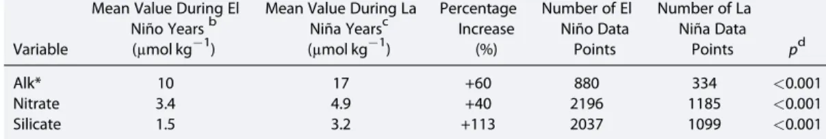
Variations in nutrients and Alk* concentrations can be observed in a meridional section across the known area of upwelling (Figure 8). The absence of a meridional increase in Alk* (decrease of 10% in the grey area in Figure 8 compared with outside the grey area (20–15°S and 10–20°N)) despite a significant increase in nitrate (increase of 490%) in the equatorial region supports hypothesis 3.2 that the upwelling is not usually from a sufficient depth to supply significant Alk*. There is also little increase in silicate concentration Table 4. T Test Results for the Effect of El Niño/La Niña Status on Properties of Surface Waters of the Eastern Equatorial Pacific^a

Variable

Mean Value During El Niño Years^b (μmol kg¹)

Mean Value During La Niña Years^c (μmol kg¹)

Percentage Increase

(%)

Number of El Niño Data Points

Number of La Niña Data

Points p^d

Alk* 10 17 +60 880 334 <0.001

Nitrate 3.4 4.9 +40 2196 1185 <0.001

Silicate 1.5 3.2 +113 2037 1099 <0.001

aTwo-sample, two-tailedttest, in the east equatorial Pacific (east of 160°W), (15°S<latitude<10°N).

bENSO index is greater than 0.5.

cENSO index is less than0.5.

dThe null hypothesis is that the mean Alk* or nutrient values from both time periods are equal; it is rejected for all three variables.

Figure 8.Surface (a) Alk* (μmol kg¹), (b) nitrate (μmol kg¹), and (c) silicate (μmol kg¹) in the eastern (east of 160°W) equatorial Pacific Ocean plotted versus latitude. The grey bar indicates the area of phenomenon 3. Values at ~5°S corre- spond to values from a short cruise into the center of the intense Chile-Peru upwelling (Figure 1).

(<1%), which indicates that the upwelled waters are derived from depths where remineralization of organic matter has supplied nitrate, but the depths are not sufficient to provide enhanced Alk* (derived from sinking calcium carbonate) and silicate (derived from sinking opal). These results can be compared to those in Table 4.

The surface concentrations of silicate and Alk* are typically low and similar to those outside the area of upwelling. However, strong upwelling during negative ENSO phases supplies waters from greater depths, increasing surface silicate and Alk*.

Thisfinding is different to that for the eastern North Pacific margin around 30°N, where upwelling has a stron- ger effect on Alk* than in the eastern equatorial Pacific. This is because the upwelled waters are older in the eastern North Pacific margin around 30°N.Feely et al.[2008] reported that the upwelled waters are derived from the potential density layer of 26.2–26.6, which has a depth of about 175 m offshore. Water at this depth has high nitrate and silicate concentrations, unlike at the equator (Figure 8 [Garcia et al., 2014b]).

In contrast to reports of a short turnover time (<10 days) for calcite in the surface ocean [Balch and Kilpatrick, 1996], there is little increase in Alk* in the surface compared with nitrate concentration (Figures 8 and 9), hence ruling against hypothesis 3.3. It is unlikely that waters high in both nitrate and Alk* are upwelled and then calcification and export rapidly remove the Alk* before the nitrate.

An increase in nitrate is apparent at around 200 m depth in the meridional section (Figure 9), whereas Alk*

increases more gradually with depth. It is therefore likely that waters are usually upwelled with enhanced nitrate concentrations but low Alk*.

In conclusion, the evidence indicates that the cause for the small average increase in Alk* from west to east (10μmol kg¹) is that the shallow depths from which waters are usually upwelled contain low concentrations of Alk* (hypothesis 3.2). The significant difference between El Niño and La Niña conditions (Table 4) indicates that stronger upwelling during La Niña years brings up deeper water, resulting in increased surface Alk*

(hypothesis 3.2). Thesefindings are similar to observations byIshii et al.[2004], who observed no increase in normalized alkalinity from west to east, possibly because the years they sampled featured positive ENSO index values (lowest ENSO index =0.21 but most months above 1).

4.4. Improved Predictive Algorithms

Our investigation shows that the enhanced Alk* in the northwestern compared with the northeastern subarc- tic Pacific at about 50°N is associated with denser isopycnals (e.g.,σθ= 27.0) reaching closer to the surface, which is probably caused by more intense Ekman pumping [Talley, 1985, 1988]. A predictive algorithm for surface alkalinity that identifies supply of deep waters should therefore improve predictive skill compared to an algorithm that does not identify recently entrained deep waters. To incorporate this mechanistic under- standing into predictive algorithms, we propose potential density (σθ), or some other measure of seawater Figure 9.Meridional sections of (a) Alk* (μmol kg¹) and (b) nitrate concentration (μmol kg¹) across the equator on WOCE cruise P18 in 1994 (along approximately 105°W). Potential density (σθ) contours are added. The black lines show the limits to the area of phenomenon 3.

density, as a predictor variable rather than temperature alone. Subsurface potential density is likely to give more accurate results because physical processes acting on the surface (e.g., evaporation, precipitation, warming, and cooling) can change the water density; however, the algorithm would be more difficult to apply if it depended on variables obtained at other depths.

Our analysis of 30°N shows that upwelling of deep waters increases surface alkalinity and highlights the diffi- culty in predicting alkalinity in regions where multiple water bodies meet, such as offshore of California and Mexico, as shown byJiang et al.[2014]. More complex algorithms should be used in order to accurately predict the alkalinity when studying this area. Previous attempts to characterize the carbonate system have been made in this region using temperature, oxygen, salinity, and potential temperature [Juranek et al., 2009;Alin et al., 2012]. However, these algorithms did not include surface waters because they are more difficult to predict.

Finally, in the equatorial Pacific we argued that the surface Alk* is affected only by the strength of upwelling as this determines the depth from which the upwelled water is derived. Because nitrate and silicate are also affected by the strength of the upwelling (as indicated by the ENSO index; e.g., see Table 4) it is possible to parameterize the variations in Alk* using more commonly measured nutrient concentrations.

Using the GLODAPv2 database, we created two algorithms using predictive equations; one algorithm of three equations covers the entire Pacific Ocean between 30°S and 65°N, and another separate algorithm, also of three equations, covers the region between 25°N and 50°N and 140°W and 110°W (Table 5).

We divided each algorithm into regions with different equations. For the basin-wide Pacific Ocean algorithm, wefirst split the basin into above or below 10°N. We then optimized the way to divide each area into two regions by sequentially splitting all the data by temperature for every degree from 0°C to 30°C and calculating the Pearson’srcorrelation coefficient (r) of a simple multiple linear regression (using nitrate, phosphate, sili- cate, salinity, potential density, and temperature) for each temperature. In the eastern North Pacific margin, we separated the areas into river influenced (salinity<32), upwelling influenced (salinity>33 and temperature<20°C), and open ocean (remaining data) as identified in section 4.2.

We transformed the nitrate, phosphate, and silicate concentrations to a normal distribution by taking natural logarithms. We transformed the other predictor variables by subtracting the mean values from salinity, potential density, and temperature (34.02, 23.4, and 21.20°C, respectively, for the Pacific Ocean algorithm or 32.76, 24.6, and 12.80°C, respectively, for the eastern margin). All subsequent analysis was performed on the transformed variables.

Table 5. Predictions of Surface Water Alkalinity in the North Pacific

Algorithm Equations^a

Measure of Algorithm Predictive Capability^b

n RMS r

Pacific Ocean^c 4541 14.1 0.970

>24°C 2246.4 + 0.20 N + 65.58 S + 2.31σθ+ 0.50σθ2 1513 7.2 0.989

≤24°C and>10°N 2281.6 + 1.93 N + 45.23 S11.98σθ+ 4.68σθ2

2623 16.9 0.910

≤24°C and≤10°N 2248.1 + 0.56 N + 67.11 S + 4.77σθ1.42σθ2 405 8.4 0.973

Sasse et al. [2013] 4 equations using salinity, temperature, oxygen, silicate, and phosphate^e 4626 12.4 0.977

Lee et al. [2006] 4 equations using salinity, temperature, and longitude^e 5773 14.2 0.969

Millero et al. [1998] 3 equations using salinity and temperature^f 5977 25.0 0.928

Eastern margin^d 477 7.03 0.991

<32 Sal 2191.2 + 2.27 N + 43.69 S19.64σθ1.55σθ2 58 8.55 0.936

>33 Sal and<20°C 2194.80.19 N + 59.19 S + 0.13σθ+ 3.77σθ2

361 6.17 0.946

Other data 2191.6 + 2.42 N + 44.22 S22.32σθ2.99σθ2 58 8.92 0.910

Sasse et al. [2013] 2 equations using salinity, temperature, oxygen, silicate, and phosphate^e 745 13.0 0.953

Lee et al. [2006] 2 equations using salinity, temperature, and longitude^e 770 22.1 0.945

Millero et al. [1998] 2 equations using salinity and temperature^f 831 27.1 0.912

aIn whichSis the salinity minus the mean (34.14 for the North Pacific and 32.76 for the eastern margin),Nis the natural logarithm of the nitrate concentration, andσθis the surface potential density minus the mean (23.2 or 24.6 for the North Pacific or eastern margin, respectively).

bnis the number of data points, RMSE is the root-mean-square error, andris the Pearson’s product moment correlation coefficient.

cFrom 30°S to 65°N and<30 m depth.

dFrom 25 to 50°N and 140 to 110°W and<30 m depth.

eEquations for the North Pacific, the (sub)tropics, the equatorial Pacific, and Southern Ocean depending on latitude, longitude, and temperature.

fEquations for the North Pacific, the gyres, and the equatorial Pacific depending on latitude, longitude, and temperature.

potential density, 1.46 for salinity, and 3.55 for silicate. We then correlated the combinations of predictor vari- ables with longitude in the subpolar North Pacific (north of 40°N) and chose to include potential density squared as it had the most significant (furthest from zero) correlation with longitude in this region (r=0.362). This value supports our conclusions in section 4.1 that the variation in Alk* is influenced by den- ser, deeper water containing dissolved calcium carbonate products. When using the predictor variables of nitrate, salinity, surface potential density, potential density squared, and silicate all the coefficients are signif- icant with a probability value smaller than 0.001, which reduces to less than 1 × 10¹⁰ when silicate is removed due to the covariance between nitrate and silicate. These probabilities indicate that all the predictor variables help to constrain alkalinity; however, there is moderate covariance between nitrate and silicate.

Table 6 summarizes the input variables and their uncertainty.

Then in each region for each algorithm, we ran a tenfold cross validation using least squares multiple linear regression both with and without silicate. This was done to produce a robustfit of the predictor variables to alkalinity. For the tenfold cross validation, we randomly split the data 10 times into two groups. Group 1 con- sisted of 90% of the data in the region, and this was used to produce the multiple linear regressions both including and excluding silicate. Group 2, containing 10% of the data in the region, was used to test the accu- racy of the equations which we measured using the root-mean-square (RMS) deviation and thercoefficient.

The inclusion of silicate did not improve thefit of the multiple linear regression, so we used the equation without it. We also increased the multiple linear regression coefficient of salinity in the northern low- temperature region to reduce the bias with longitude. This increased the RMS; however, it also increased therin the region. Thefinal statistical results were then compared with previously reported algorithms by Millero et al.[1998],Lee et al.[2006], andSasse et al.[2013] using the GLODAPv2 database (Table 5).

Our prediction for the Pacific Ocean accounts for more variability than the algorithms byLee et al.[2006]

andMillero et al.[1998] but not more than the algorithm bySasse et al.[2013]. For the entire Pacific, the rof our algorithm is 0.970 compared to 0.928, 0.969, and 0.977 for algorithms byMillero et al.[1998],Lee et al.[2006], andSasse et al.[2013], respectively, and the RMS of our algorithm is 14.1μmol kg¹compared to 25.0, 14.2, and 12.4μmol kg¹ for algorithms byMillero et al.[1998],Lee et al.[2006], andSasse et al.

[2013], respectively.

The algorithm for the whole Pacific is also an improvement in terms of simplicity; it uses only three equations to cover the Pacific Ocean north of 30°S, rather than the four equations used byLee et al.[2006] andSasse et al.[2013]. The ability to make predictions of similar accuracy (first two significantfigures of thervalue are the same) as previous attempts, with fewer equations, and without using longitude as an artificial predic- tor as used byLee et al.[2006], suggests that our algorithm corresponds more closely to the underlying mechanistic reality. Because our algorithm for the Pacific Ocean has fewer equations, it is also simpler and therefore easier to apply.

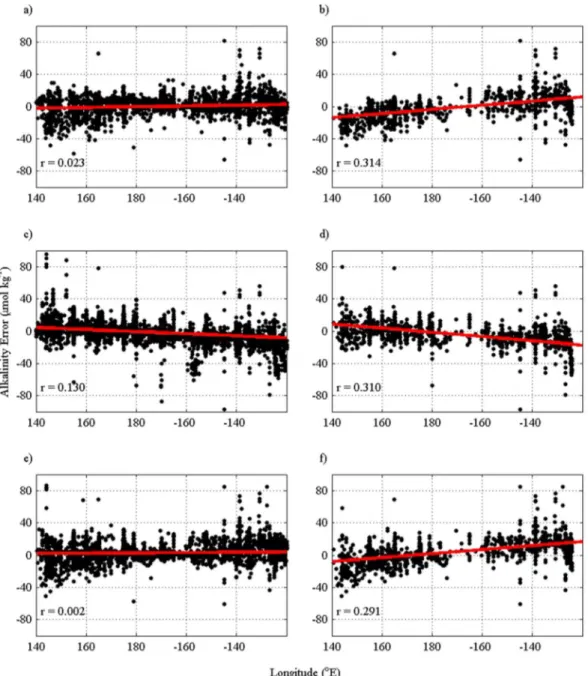
Residuals for our Pacific Ocean algorithm show no relationship with year (R²= 0.020,N= 860) or with ENSO index (R²= 0.014,N= 860) in equatorial waters, showing that it performs well in both El Niño and La Niña years. Our Pacific Ocean algorithm, without longitude as a predictor variable, is not biased (r= 0.002, N= 4541) with longitude for the whole area (Figure 10e). But, the same algorithm applied in the subpolar North Pacific is biased (r= 0.291,N= 1662) with longitude (Figure 10f). However, thervalue (Alk* residual ver- sus longitude) is less than that for both the algorithms bySasse et al.[2013] and byLee et al.[2006]. When

using theLee et al.[2006] algorithm, the residuals (Figures 10c and 10d) increase from east to west even in the subpolar North Pacific where longitude was used as an additional variable to reduce this bias.

Figure 11 shows the relationship between the residuals and longitude in the areas of each of the phenomena.

The subpolar North Pacific (45–55°N) has the strongest bias (r= 0.635) with longitude despite the use of squared potential density and an increased salinity coefficient to specifically reduce bias in this region.

This bias is still less than the bias of theSasse et al.[2013] algorithm in the same region (r= 0.874). The result- ing gradient in the residuals from west to east is an increase of 19μmol kg¹, which is 4μmol kg¹less than the magnitude of the original gradient in alkalinity in the subpolar North Pacific. The increase from west to east is because our algorithm underpredicts in the high alkalinity north-west and overpredicts in the lower alkalinity north-east. The direction of our bias is similar to the bias from the algorithm bySasse et al.[2013]

but opposite to the algorithm byLee et al.[2006], which underpredicts the low alkalinity in the west. We Figure 10.Predicted alkalinity minus measured alkalinity from theSasse et al.[2013] algorithm in (a) the entire Pacific Ocean (north of 30°S) and (b) the high-latitude subarctic North Pacific (north 40°N). (c and d) The same areas using the algorithm byLee et al.[2006] and (e and f) the same areas using our algorithm for the entire Pacific Ocean algorithm. The solid red lines are the bestfit straight lines.

5.3μmol kg¹), and the residuals along the equator increase by 0.56μmol kg¹(from0.6μmol kg¹ to0.04μmol kg¹). These statistics show little bias, and therefore, our entire Pacific Ocean algorithm models the natural variation in these regions.

For the eastern margin, our algorithm is more accurate than previous algo- rithms; the r increased from 0.912, 0.945, and 0.953 (for the algorithms byMillero et al.[1998],Lee et al.[2006], andSasse et al.[2013], respectively) to 0.991, and RMS error decreased from 27.1, 22.1, and 13.0μmol kg¹to 7.03μmol kg¹. This is partly because our algorithm is designed spe- cifically for the area, whereas the others were not.

4.5. Possible Future Changes in Alkalinity

An improved mechanistic understanding of carbonate chemistry in the North Pacific will be helpful for esti- mating future changes in alkalinity and calcium carbonate saturation state. There is evidence that climate change is causing winds to strengthen, which may increase upwelling along the North American coast [Bakun, 1990;Hauri et al., 2013;Sydeman et al., 2014]. Upwelled waters in this area have enhanced Alk* from dissolution of calcium carbonate minerals at depth (Figure 6); therefore, future increases in wind strength could cause a local increase in Alk*. Changes in ocean circulation could also affect alkalinity concentrations in the equatorial Pacific; climate change may cause El Niño conditions to occur more frequently by strength- ening of the equatorial thermocline [Timmermann et al., 1999;Yeh et al., 2009]. Because upwelling of alkalinity seems to occur only during La Niña events, if they occur less frequently in future then it is likely that less alka- linity will be upwelled in the equatorial Pacific.

5. Conclusions

Analysis of data from GLODAPv2 and other data sets allowed us to test a series of hypotheses on the causes of longitudinal variations in Alk* in the North Pacific. At 50°N, the major cause of variation was found to be denser isopycnals (with higher Alk*) coming closer to the surface on the western side. At about 30°N, the higher Alk*

close to the eastern margin is caused predominantly by upwelling off the North American continent. But in the eastern equatorial Pacific, upwelling does not increase the surface Alk* to significantly higher than in the west.

Alk* is, however, higher in the east during La Niña years, probably because stronger upwelling during these periods brings water to the surface from greater depths, depths at which Alk* is elevated.

We created two algorithms (entire Pacific Ocean and eastern margin of the North Pacific) to predict alkalinity using salinity, nitrate, and potential density. The Pacific Ocean algorithm is of similar accuracy to the best pre- vious algorithm bySasse et al.[2013] (rvalue of 0.970 for our algorithm versus 0.977 for their algorithm).

However, our algorithm is less biased with longitude in the subpolar North Pacific (north of 40°N) with anr Figure 11.Residual alkalinity (predicted alkalinity minus measured alkali-

nity) using the Pacific Ocean algorithm in (a) the region of phenomenon 1 (45–55°N), (b) the region of phenomenon 2 (25–40°N), and (c) the region of phenomenon 3 (15°S–10°N).

value of 0.291 between the residuals and longitude compared to 0.314 bySasse et al.’s [2013] algorithm. Our algorithm for the eastern margin of the North Pacific is more accurate than previously published algorithms (r= 0.991 compared to 0.953 fromSasse et al.[2013]).

References

Alin, S. R., R. A. Feely, A. G. Dickson, J. M. Hernández-Ayón, L. W. Juranek, M. D. Ohman, and R. Goericke (2012), Robust empirical relationships for estimating the carbonate system in the southern California Current System and application to CalCOFI hydrographic cruise data (2005–2011),J. Geophys. Res.,117, C05033, doi:10.1029/2011JC007511.

Amiotte Suchet, P., J.-K. Probst, and W. Ludwig (2003), Worldwide distribution of continental rock lithology: Implications for the atmospheric/soil CO2uptake by continental weathering and alkalinity river transport to the oceans,Global Biogeochem. Cycles,17(2), 1038, doi:10.1029/2002GB001891.

Bakun, A. (1990), Global climate change and intensification of coastal ocean upwelling,Science,247, 198–201, doi:10.1126/

science.247.4939.198.

Balch, W. M., and K. Kilpatrick (1996), Calcification rates in the equatorial Pacific along 140°W,Deep Sea Res., Part II,43(4–6), 971–993, doi:10.1016/0967-0645(96)00032-X.

Bond, N. A., J. E. Overland, M. Spillane, and P. Stabeno (2003), Recent shifts in the state of the North Pacific,Geophys. Res. Lett.,30(23), 2183, doi:10.1029/2003GL018597.

Brewer, P. G., and J. C. Goldman (1976), Alkalinity changes generated by phytoplankton growth,Limnol. Oceanogr.,21(1), 108–117, doi:10.4319/lo.1976.21.1.0108.

Cai, W.-J., X. Hu, W.-J. Huang, L.-Q. Jiang, Y. Wang, T.-H. Peng, and X. Zhang (2010), Alkalinity distribution in the western North Atlantic Ocean margins,J. Geophys. Res.,115, C08014, doi:10.1029/2009JC005482.

Cai, W.-J., et al. (2011), Acidification of subsurface coastal waters enhanced by eutrophication,Nat. Geosci.,4(11), 766–770, doi:10.1038/

ngeo1297.

Chen, C.-T. A. (1996), The Kuroshio intermediate water is the major source of nutrients on the East China Sea continental shelf,Oceanol. Acta, 19(5), 523–527.

Chen, C.-T. A. (2002), Shelf-vs. dissolution-generated alkalinity above the chemical lysocline,Deep Sea Res. Part II Top. Stud. Oceanogr., 49(24–25), 5365–5375, doi:10.1016/S0967-0645(02)00196-0.

Chen, C.-T. A., and R. M. Pytkowicz (1979), On the total CO2-tritation alkalinity oxygen system in the Pacific Ocean,Nature,281, 362–365, doi:10.1038/281362a0.

Chen, C.-T. A., and S.-L. Wang (1999), Carbon, alkalinity and nutrient budgets on the East China Sea continental shelf,J. Geophys. Res.,104, 20,675–20,686, doi:10.1029/1999JC900055.

Chen, G.-T., and F. J. Millero (1979), Gradual increase of oceanic CO2,Nature,277, 205–206, doi:10.1038/277205a0.

Cummins, P. F., and H. J. Freeland (2007), Variability of the North Pacific Current and its bifurcation,Prog. Oceanogr.,75(2), 253–265, doi:10.1016/j.pocean.2007.08.006.

Dahm, C. N., S. V. Gregory, and P. Kilho Park (1981), Organic carbon transport in the Columbia River,Estuarine Coastal Shelf Sci.,13, 645–658, doi:10.1016/S0302-3524(81)80046-1.

de Mora, S. J. (2008), The distribution of alkalinity and pH in the Fraser estuary,Environ. Technol. Lett.,4(1), 35–46, doi:10.1080/

09593338309384169.

Di Lorenzo, E., et al. (2008), North Pacific Gyre Oscillation links ocean climate and ecosystem change,Geophys. Res. Lett.,35, L08607, doi:10.1029/2007GL032838.

Dickson, A. G., J. D. Afghan, and G. C. Anderson (2003), Reference materials for oceanic CO2analysis: A method for the certification of total alkalinity,Mar. Chem.,80, 185–197, doi:10.1016/S0304-4203(02)00133-0.

Douglass, E., D. Roemmich, and D. Stammer (2006), Interannual variability in northeast Pacific circulation,J. Geophys. Res.,111, C04001, doi:10.1029/2005JC003015.

Dyrssen, D., and L. G. Sillén (1967), Alkalinity and total carbonate in sea water. A plea forp-T-independent data,Tellus A,1, 113–121, doi:10.3402/tellusa.v19i1.9755.

Elvert, M., E. Suess, J. Greinert, and M. J. Whiticar (2000), Archaea mediating anaerobic methane oxidation in deep-sea sediments at cold seeps of the eastern Aleutian subduction zone,Org. Geochem.,31, 1175–1187, doi:10.1016/S0146-6380(00)00111-X.

Feely, R. A., C. L. Sabine, J. M. Hernandez-Ayon, D. Ianson, and B. Hales (2008), Evidence for upwelling of corrosive“acidified”water onto the continental shelf,Science,320, 1490–1492, doi:10.1126/science.1155676.

Friis, K., A. Körtzinger, and D. W. R. Wallace (2003), The salinity normalization of marine inorganic carbon chemistry data,Geophys. Res. Lett., 30(2), 1085, doi:10.1029/2002GL015898.

Fry, C. H., T. Tyrrell, M. P. Hain, N. R. Bates, and E. P. Achterberg (2015), Analysis of global surface ocean alkalinity to determine controlling processes,Mar. Chem.,174, 46–57, doi:10.1016/j.marchem.2015.05.003.

Garcia, H. E., R. A. Locarnini, T. P. Boyer, J. I. Antonov, O. K. Baranova, M. M. Zweng, J. R. Reagan, and D. R. Johnson (2014a), Volume 2: Dissolved oxygen, apparent oxygen utilization, and oxygen saturation, inWorld Ocean Atlas 2013,NOAA Atlas NESDIS 75, edited by S. Levitus and A.

Mishonov, pp. 27, Silver Spring, Md.

Garcia, H. E., R. A. Locarnini, T. P. Boyer, J. I. Antonov, O. K. Baranova, M. M. Zweng, J. R. Reagan, and D. R. Johnson (2014b), Volume 4: Dissolved inorganic nutrients (phosphate, nitrate, silicate), inWorld Ocean Atlas 2013,NOAA Atlas NESDIS 76, edited by S. Levitus and A. Mishonov, pp. 25, Silver Spring, Md.

Hauri, C., N. Gruber, M. Vogt, S. C. Doney, R. A. Feely, Z. Lachkar, A. Leinweber, A. M. P. McDonnell, M. Munnich, and G.-K. Plattner (2013), Spatiotemporal variability and long-term trends of ocean acidification in the California Current System,Biogeosciences,10, 193–216, doi:10.5194/bg-10-193-2013.

Hein, J. R., J. R. O’Neil, and M. G. Jones (1979), Origin of authigenic carbonates in sediment from the deep Bering Sea,Sedimentology,26, 681–705, doi:10.1111/j.1365-3091.1979.tb00937.x.

Huyer, A. (1983), Coastal upwelling in the California Current System,Prog. Oceanogr.,12, 259–284, doi:10.1016/0079-6611(83)90010-1.

Ishii, M., S. Saito, T. Tokieda, T. Kawano, K. Matsumoto, and H. Y. Inoue (2004), Variability of surface layer CO2parameters in the western and central equatorial Pacific, inGlobal Environmental Change in the Ocean and on Land, edited by M. Shiyomi et al., pp. 59–94, Terrapub, Tokyo.

Acknowledgments

We thank all those who contributed to the collection, analysis, and synthesis of the GLODAPv2. The data used in this paper are referenced. This study was financially supported by a NERC doc- toral training grant to C.H. Fry (NE/

K500926/1).

slope sediment,Deep Sea Res., Part I,49(10), 1837–1852, doi:10.1016/S0967-0637(02)00092-4.

Millero, F. J., K. Lee, and M. Roche (1998), Distribution of alkalinity in the surface waters of the major oceans,Mar. Chem.,60, 111–130, doi:10.1016/S0304-4203(97)00084-4.

Monterey, G., and S. Levitus (1997),Seasonal Variability of Mixed Layer Depth for the World Ocean, U.S. Government Printing Office, Washington D. C.

Olsen, A., et al. (2016), An internally consistent data product for the world ocean: The Global Ocean Data Analysis Project, version 2 (GLODAPv2),Earth Syst. Sci. Data Discuss., 1–78, doi:10.5194/essd-2015-42.

Park, P. K., G. R. Webster, and R. Yamamoto (1969), Alkalinity budget of the Columbia River,Limnol. Oceanogr.,14(4), 559–567.

Sasse, T. P., B. I. McNeil, and G. Abramowitz (2013), A novel method for diagnosing seasonal to inter-annual surface ocean carbon dynamics from bottle data using neural networks,Biogeosciences,10(6), 4319–4340, doi:10.5194/bg-10-4319-2013.

Sydeman, W. J., M. García-Reyes, D. S. Schoeman, R. R. Rykaczewski, S. A. Thompson, B. A. Black, and S. J. Bograd (2014), Climate change and wind intensification in coastal upwelling ecosystems,Science,345, 77–80, doi:10.1126/science.1251635.

Takatani, Y., K. Enyo, Y. Iida, A. Kojima, T. Nakano, D. Sasano, N. Kosugi, T. Midorikawa, T. Suzuki, and M. Ishii (2014), Relationship between total alkalinity in surface water and sea surface dynamic height in the Pacific Ocean,J. Geophys. Res. Ocean.,199, 2806–2814, doi:10.1002/

2013JC009739.

Talley, L. D. (1985), Ventilation of the subtropical North Pacific: The shallow salinity minimum,J. Phys. Oceanogr.,15, 633–649, doi:10.1175/

1520-0485(1985)015<0633:VOTSNP>2.0.CO;2.

Talley, L. D. (1988), Potential vorticity distribution in the North Pacific,J. Phys. Oceanogr.,18, 89–106, doi:10.1175/1520-0485(1988)018<0089:

PVDITN>2.0.CO;2.

Timmermann, A., J. Oberhuber, A. Bacher, M. Esch, M. Latif, and E. Roeckner (1999), Increased El Niño frequency in a climate model forced by future greenhouse warming,Nature,398, 694–697, doi:10.1038/19505.

Tsunogai, S., S. Watanabe, J. Nakamura, T. Ono, and T. Sato (1997), A preliminary study of carbon system in the east,J. Oceanogr.,53, 9–17, doi:10.1007/BF02700744.

Wolf-Gladrow, D. A., R. E. Zeebe, C. Klaas, A. Körtzinger, and A. G. Dickson (2007), Total alkalinity: The explicit conservative expression and its application to biogeochemical processes,Mar. Chem.,106(1–2), 287–300, doi:10.1016/j.marchem.2007.01.006.

Xie, S.-P., and S. G. H. Philander (1994), A coupled ocean-atmosphere model of relevance to the ITCZ in the eastern Pacific,Tellus A,46, 340–350, doi:10.3402/tellusa.v46i4.15484.

Yeh, S.-W., J.-S. Kug, B. Dewitte, M.-H. Kwon, B. P. Kirtman, and F.-F. Jin (2009), El Niño in a changing climate,Nature,461, 511–514, doi:10.1038/nature08316.