Generalized Satisﬁability Problems

(1)

Generalized Satisfiability Problems

Dissertation zur Erlangung des naturwissenschaftlichen Doktorgrades

der Bayerischen Julius-Maximilians-Universit¨at W¨urzburg

vorgelegt von

Steffen Reith

aus

W¨urzburg

W¨urzburg, 2001

(2)

1. Gutachter: Prof. Dr. Klaus W. Wagner 2. Gutachter: Prof. Dr. Nadia Creignou Tag der m¨undlichen Pr¨ufung: 16. 07. 2001

(3)

Ich möchte allen danken, die mit Rat, Unterstützung und Hilfe dazu beigetra- gen haben, dass diese Arbeit gedeihen konnte. Insbesondere möchte ich Klaus W. Wagner danken, der mir diese Arbeit ermöglichte. Auch meinen Freunden und Kollegen Herbert Baier, Elmar Böhler, Helmut Celina, Matthias Galota, Sven Kosub und Heribert Vollmer möchte ich für die vielen Diskussionen, Ideen, Tipps, Hilfen und Aufmunterungen danken, ohne die diese Arbeit nie entstanden wäre.

(4)

(5)

F¨ur Christiane

(6)

(7)

List of Figures

2.1 The polynomial time hierarchy and some other important complexity

classes. . . 20

2.2 Graph of all classes of Boolean functions being closed under superposition. 24 2.3 Some Boolean functions and their dual function. . . 26

3.1 A polynomial-time algorithm for VAL^C(B). . . 34

3.2 All closed classes of Boolean functions containing id, 0, and 1. . . 35

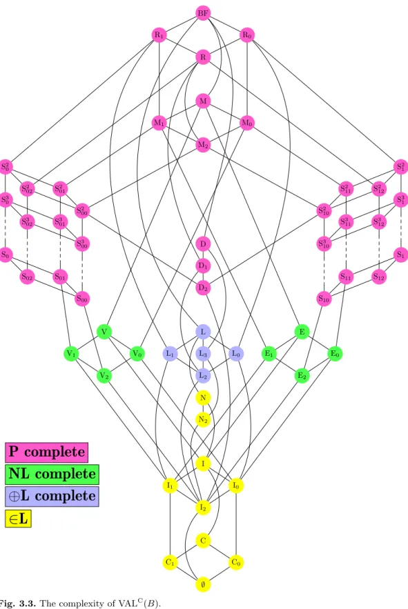
3.3 The complexity of VAL^C(B). . . 37

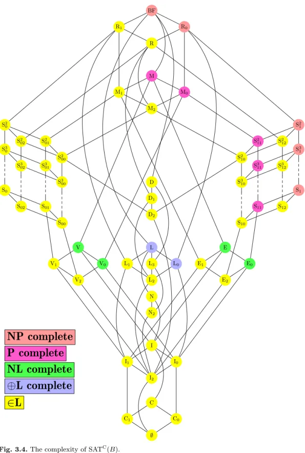
3.4 The complexity of SAT^C(B). . . 41

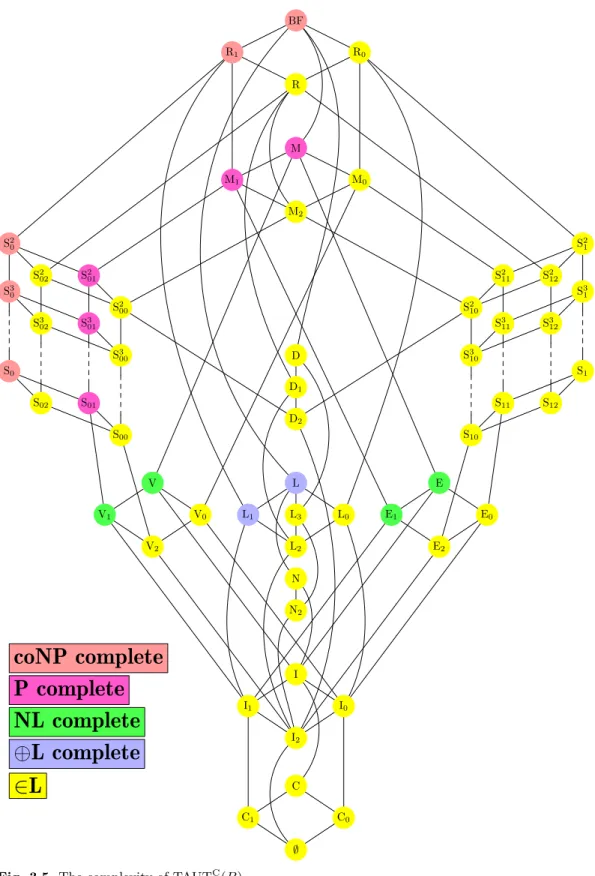
3.5 The complexity of TAUT^C(B). . . 43

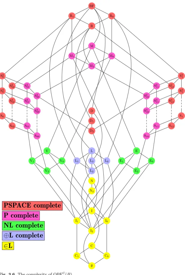
3.6 The complexity of QBF^C(B). . . 47

3.7 The complexity of THR^C(B). . . 54

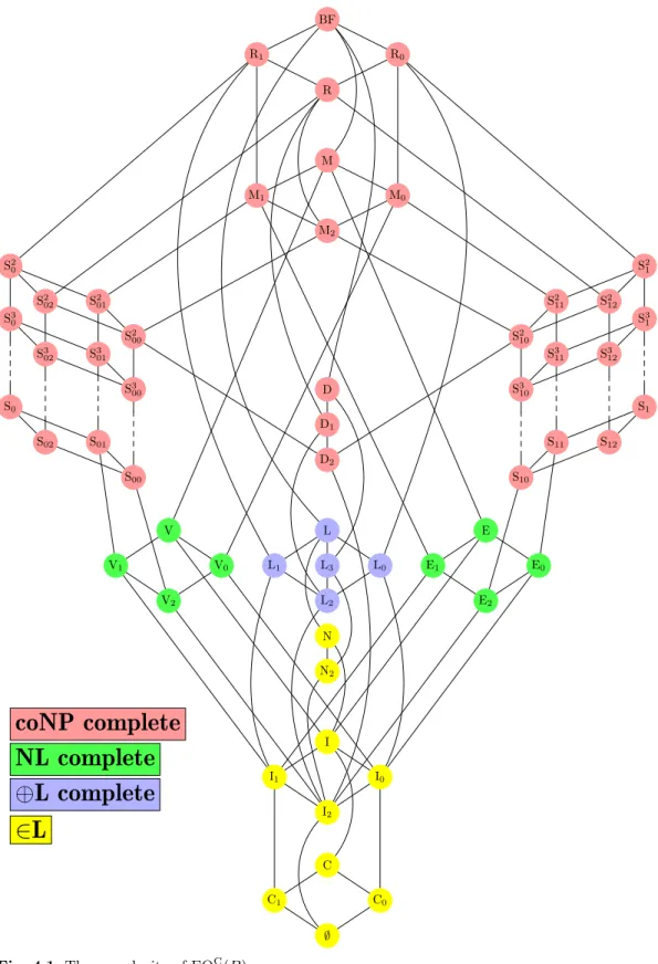
4.1 The complexity of EQ^C(B). . . 74

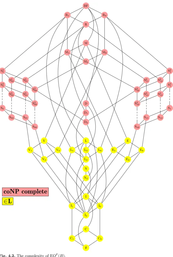
4.2 The complexity of EQ^F(B). . . 75

5.1 An algorithm to calculate the lexicographically minimal satisfying assignment. . . 80

5.2 The complexity of LexMinSAT(B). . . 84

5.3 The complexity of LexMaxSAT(B). . . 86

(10)

(11)

1. Overview

In the last 40 years, complexity theory has grown to a rich and powerful field in theoretical computer science. The main task of complexity theory is the classifi- cation of problems with respect to their consumption of resources (e.g., running time, required memory or number of needed processors).

To study the computational complexity (i.e., consumption of resources) of problems, all “similar” problems are grouped into a “complexity class”. The main intention behind this is the hope to get a better insight into the common properties of these problems and therefore to obtain a better understanding of why some problems are easy to solve, whereas for others practical algorithms are either not known or are even proven not to exist.

Clearly, when we want to measure the consumption of resources which are needed to solve a problem, we have to talk about the computing device we want to use. In the history of complexity theory, the Turing-machine in various modifications has proven to be a good, robust, and realistic model for this task. Hence all results in this thesis are based on Turing-machines as computational devices.

Everybody who is familiar with the task of finding an algorithm for a given problem is aware of the following dilemma: Often one is able to find a suitable algorithm very fast, others are trickier to find. In some other cases no fast algorithm is known despite tremendous efforts to find one. This led to the situation that by 1970, many problems with no known fast algorithm had been discovered, and it was unknown, whether fast algorithms either did not exist or whether so far nobody had been clever enough to find one.

A major breakthrough in this situation was the introduction of the complexity classes P and NP, which were introduced by Stephan A. Cook in 1971 (cf. [Coo71]). (Implicitly Leonid Levin achieved the same results independently in [Lev73].) WhileP is the class of problems which can be solved efficiently, i.e., in polynomial time, the class NP consists of all problems which can be solved by a non deterministic Turing-machine in polynomial time. Today the class P is used as a “definition” of computational “easiness” or “tractability”; we call a problem, which is solvable in polynomial time by a deterministic Turing-machine

“easy”, whereas all other problems are called “intractable”. Hence the classesP and NPare of immense importance.

The problem whether these two classes coincide or differ is known nowadays as the famousP=^? NP problem. Nearly everybody who is aware of the basics of algorithms is familiar with this problem, showing that it has a huge influence on

(12)

all aspects of theoretical computer science and especially on complexity theory.

Therefore it is not astonishing, that nearly all results in complexity theory are related to this question and also the present thesis is connected to the P =^? NP problem.

Interestingly, the P =^? NP problem has a history at least reaching back to 1956, when G¨odel sent a letter to von Neumann, in which he stated the following problem:

Given a first-order formula¹ F and a natural numbern, determine if there is a proof of F of length n.

G¨odel was interested in the number of steps needed by a Turing-machine to solve this problem and asked whether there is an algorithm for this problem running in linear or quadratic time².

Nowadays, a problem which is closely related to G¨odel’s problem is known as SAT and is used in varying contexts of complexity theory. Moreover SAT was identified by Cook as an example for a problem which is most likely not solvable by any polynomial time algorithm. To justify this statement, he proved the completeness of SAT for NP, which means that SAT is one of the hardest problems in the class NP. To classify problems in NP we have to compare them with all other problems inNP. As a tool for comparing the computational complexity of problems Cook introduced the concept ofreductions. The intention behind reduc- tions is to partially order problems (out ofNP) with respect to the computational power needed to solve them. Informally, a reduction compares the complexity of two problems in the following way: a problem A can be reduced to a problemB if there is an easy transformation which converts an inputx for A into an inputx⁰ for B and x belongs to A iff x⁰ belongs to B. This means that we can solve A with the help of B and the easy transformation, hence B cannot be easier than A. If we are able to find a problem inside NP, which has the property that it is not easier than any other problem inNP, then this problem is one of the hardest in NP. In Cook’s terminology such a problem is called NP-complete and has a very special property: If we are able to find a polynomial time algorithm for an NP-complete problem, then P= NP and if we are able to show that P6= NP then we know that there cannot exist an efficient method for solving such anNP- complete problem. Because of this property we can imagine that we have distilled all substantial properties from all problems of NP into one problem. This fact makesNP-complete problems so important for complexity theory.

Another important way of looking at theP=^? NPproblem comes from proof- theory. It is known that Pcan be considered as the class of all problems A such that, for any inputx forA, we can find aproof orwitness for the membership of x efficiently, if x ∈ A holds. On the other hand, NP is the class of all problems

1 Formel des “engeren Funktionenkalk¨uls”.

2 Such an algorithm would mean “dass die Anzahl der Schritte gegen¨uber dem blossen Probieren von N auf logN (oder (logN)²) verringert werden kann”.

(13)

1. Overview 13

B such that there exists a short proof of membership, which can be checked efficiently. Take as an example the problem SAT. The input of this problem is a propositional formula H. If H ∈ SAT we know that there is an assignment of all variables occurring in H, such that this assignment satisfies H. Since we can efficiently check for an arbitrary assignment whether it satisfies a given formula or not, the existence of a satisfying assignment is a proof of the membership ofH to SAT. Since such an assignment is short with respect to the length of the formula H, this shows that SAT belongs to NP. In contrast to this use the problem HORN-SAT, where we have to check the existence of a satisfying assignment of a Horn-formula. There exists a well known fast algorithm to determine a satisfying assignment of a Horn-formula iff one exists (see [Pap94]), hence a witness for H ∈ HORN-SAT can be easily computed, showing that HORN-SAT belongs to the classP.

But the concept of NP-completeness is also important for the design of algorithms. If we can prove that a given problem isNP-complete, we have shown that all known tools for designing algorithms cannot help us to manage it, because nobody was able to showP=NPup to now. Moreover, it is likely that we will never find an efficient algorithm, because it is widely believed in complexity theory that P 6= NP. The importance for practical purposes is supported by a steadily growing list of NP-complete problems, which belong to logics, network- ing, storage and retrieval, graph theory, algebra, and number theory. An early collection of more than 300 NP-complete problems can be found in [GJ79].

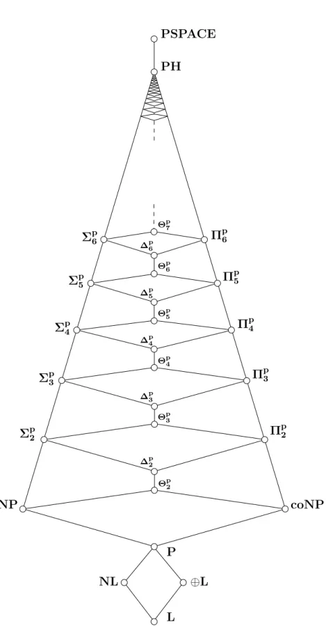
In complexity theory, the study of NP led to numerous related classes, e.g., the classes of the polynomial-time hierarchy PH, PP, L, #P, and #L. (For a diagram showing some inclusional relationships see Fig. 2.1.) The concept of completeness is not only restricted to the class NP. Less well known as NP- complete problems, there are also many P-complete problems examined today.

Many of these problems are related to Boolean formulas and Boolean circuits, e.g., the problem of finding a satisfying assignment of a Horn-formula, which plays an important role in the theory of databases and programming languages. A source of P-complete problems having a similar intention as [GJ79] is [GHR95]. Today we know complete problems for subclasses ofP, like NL, ⊕L and L, too.

As mentioned above, Cook showed that SAT is an NP-complete problem and various modifications and restrictions of SAT were used to show completeness results, not only for NP, but, e.g., for P, NL, ⊕L, PP, Σ^p_k, and #P. Hence some questions arise: Why is SAT so hard to solve? Are there restrictions of SAT which are not so hard to solve? Can we prove that these restricted versions of SAT are complete for well-known subclasses of NP? And the other way around: How do we have to generalize the SAT-problem to obtain completeness results beyond NP, maybe for the classes of the polynomial time hierarchy, PP orPSPACE?

And finally: Do the results for circuits and formulas differ? The present work will focus on these questions.

(14)

Boolean functions

In the 1920s, Emil Leon Post extensively studied Boolean functions. Almost twenty years later he published his work in [Pos41], where he presented his results comprehensively. Today these superb results are not widely known and the only other source for his results is the monograph [JGK70], which is a German translation of a Russian original, giving a summary of [Pos41]. One of his main outcomes was the identification of all closed sets of Boolean functions, showing that all those classes are generated by a finite base. For this, he used the super- position of Boolean functions as the operation to combine them, where we are allowed to identify, permute, and substitute variables to construct a new function.

Intuitively, this is the same as combining Boolean functions by soldering inputs and outputs together, forming a new Boolean function.

This impressive result is not widely known, but the resulting completeness test for Boolean functions can be found in basic textbooks about theoretical computer science (e.g., [Wag94]). We call a set of Boolean functionscomplete iff its closure under superposition is the set of all Boolean functions. Post showed that there are five maximal closed classes of Boolean function; these are circled bold in Figure 2.2 (these maximal closed classes are known as “Post’s classes”). Hence we know that a set of Boolean functions, which does not belong to any of these five classes, must be a complete set (cf. Corollary 2.10).

Generalized propositional formulas and circuits

When we define propositional formulas inductively, we start with propositional variables. In the induction step, we are allowed to combine smaller propositional formulas with connector symbols. It is common to use symbols for the Boolean and, or and not function, since it is known that all Boolean functions can be represented in this way. Similarly, this technique is used to introduce Boolean circuits. The only difference between circuits and formulas is that circuits have the structure of an acyclic directed graph, whereas we restrict formulas to a tree-like form. We will see later that this restriction of formulas leads to different results in some cases. Now it is natural to generalize circuits and formulas in the following way: We are allowed to use connection symbols which represent Boolean functions out of a fixed set B of Boolean functions. Later we will use the term B-circuit or B-formula for these generalized Boolean formulas and circuits. Moreover, we will see that B-circuits and B-formulas represent all Boolean functions out of the closure under superposition ofB. Because of this, we can make use of Post’s results to study our generalized circuits and formulas. Since all closed sets of Boolean functions are known, we are able to give results about “all definable generalized propositional logics” by varying the used set B. Similarly, we are able to study problems related to circuits built over arbitrary bases, i.e., sets of Boolean functions used as gate-types (cf. Chapter 3 and Chapter 4).

(15)

1. Overview 15

Boolean constraint satisfaction problems

Let us start with a prototypical example for constraint satisfaction problems.

3 -SAT is a very well-known restriction of SAT, which is still NP-complete. Here we have to search for satisfying assignments of a propositional formula in conjunc- tive normal form, i.e., all inputs are of the formC1∧C2∧ · · · ∧Cm, where eachCi

(clause) consists of a disjunction of Boolean variables, which might be negated.

Hence a satisfying assignment has to fulfill each clause in parallel. Therefore, each clause is called a “constraint” for our overall solution. But such clauses are not very general and they are hardly useful to model “natural” constraints. To over- come this restriction, in 1978, Thomas Schaefer invented a strong generalization of this concept. He replaced the clauses with an arbitrary Boolean predicate out of a fixed set S and called the resulting formulas S-formulas. Now it is easy to define satisfiability problems, like, e.g., EXACTLY-ONE-IN-THREE-SAT, where we require that a satisfying assignment assigns exactly one variable of each clause to true. While studying this kind of formulas, he gave a broad criterion to de- cide the complexity of this family of satisfiability problems and was able to show that the complexity only depends on the used set of predicates. Very surprisingly, Schaefer proved that the satisfiability problem forS-formulas is either decideable inP or complete for NP. Hence he called this theorem a dichotomy theorem for generalized constraint satisfaction. This is an interesting, surprising, and not very obvious property, because Ladner showed in [Lad75] that there are infinitely many degrees between P and NP, under the assumption that P6=NP, hence there is no evident reason why none of Schaefers problems can be found in one of these in- termediate degrees. Influenced by Schaefers results, many other problems related to S-formulas were studied (see [Cre95, CH96, KST97, KSW97, CKS99, KK01]

and Section 5.4.), leading to a wealth of completeness results for e.g.,PSPACE,

#P, and MAXSNP. Following this branch of complexity theory, in Section 5.4 we will study the problem of finding the smallest (largest, resp.) satisfying assignment of an S-formula.

A short summary

In Chapter 2 we will give a short introduction into the topics of complexity theory which will be needed here. For a comprehensive introduction into complexity theory see [Pap94, BDG95, BDG90]. After that we advance to Boolean functions and give a short summary about closed classes of Boolean functions.

This section heavily hinges on results achieved by Emil Leon Post already in the twenties of the 20^th century (see [Pos41]). We finish this chapter with the introduction of generalized Boolean circuits and formulas and some basic notations for them.

In Chapter 3 we will study various problems related to generalized Boolean circuits and formulas. First we will study the circuit value problem for generalized Boolean circuits in Section 3.2, since it plays a central role for all other problems

(16)

which will be considered in this work. After that we will completely classify the satisfiability and tautology problem for generalized circuits, which leads various completeness results forNP,coNPand classes below them (cf. Section 3.3). As a natural generalization we will study quantified generalized Boolean circuits in Section 3.4 and obtain results for quantified circuits having a bounded or un- bounded number of quantifiers. Additionally there can be found results about the complexity of determining the number of satisfying assignments of generalized circuits and of checking whether a given circuit has more than k satisfying assignments. At the end of this chapter we present a beautiful result by Harry Lewis about generalized formulas and we use it to study the satisfiability problem related to B-formulas.

In Chapter 4 we will present results for the equivalence problem and the iso- morphism problem of B-circuits and B-formulas. This means that we completely clarify the complexity whether two given circuits or formulas represent the same Boolean function. In the isomorphism case, this is beyond the means of present techniques, hence in some cases we only give lower bounds, which are as good as the trivial lower bounds known for the unrestricted isomorphism problem.

Finally in Chapter 5 we study the complexity of finding the lexicographically smallest and largest satisfying assignment for a given generalized formula. In contrast to the other chapters we study two different kinds of formulas, namely B-formulas andS-formulas. After a brief introduction into relevant known results, we turn to the generalized formulas in the Post context. After that we conclude with formulas initially introduced by Thomas Schaefer in [Sch78].

Finally note that Chapter 3 is based on [RW00] and that Chapter 5 was published in [RV00]. The material which will be presented in Chapter 4 was not published before.

(17)

2. Basics

2.1 Complexity theory

In this section we will informally introduce some standard notations and results from complexity theory. For more details see [BDG95, BDG90, Pap94].

The complexity classes P, NP, L, NL, and PSPACE are defined as the classes of languages (problems) which can be accepted by deterministic polynomially time bounded Turing-machines, nondeterministic polynomially time bounded Turing-machines, deterministic logarithmically space bounded Turing-machines, nondeterministic logarithmically space bounded Turing-machines, and deterministic polynomially space bounded Turing-machines, resp. Let PP be the class of languages which can be accepted by a nondeterministic polynomially time bounded Turing-machineM in the following manner: An input (x, k) is accepted byM iff more thank of M’s computation paths on input xare accepting paths.

Let ⊕L be the class of languages which can be accepted by a nondeterministic logarithmically space bounded Turing-machine M in the following manner: An input x is accepted by M iff the number of M’s accepting paths on input x is odd.

Following the notation from [BDG95, BDG90] we use a generic notation for time- and space-bounded classes of problems, which can be solved by deterministic and nondeterministic multi-tape Turing-machines;DTIME(s),DSPACE(s), NTIME(s) and NSPACE(s), where s: N → N is the given bound for time or space. NowL=DSPACE(logn),NL=NSPACE(logn),P=DTIME(nÔ(1)), NP=NTIME(nÔ(1)) and PSPACE=DSPACE(nÔ(1)).

For a class K of languages let coK =def {A | A ∈ K}. Furthermore let P^K, NP^K,L^K, andNL^K be the classes of languages accepted by the type of machines used for the classes P, NP, L, and NL, resp., but which have the additional ability to ask queries to languages from K free of charge (such machines are called oracle Turing machines). If we want to restrict the number of queries to s, we will write P^K[s], NP^K[s],L^K[s], and NL^K[s].

The classes of the polynomial time hierarchy are inductively defined as follows: Σ^p₀ = Π^p₀ = Θ^p₀ = ∆^p₀ =def P. For k ≥ 1 we define Σ^p_k =def NP^Σ^p^k⁻¹, Π^p_k =def coΣ^p_k = coNP^Σ^p^k⁻¹, Θ^p_k =def P^Σ^p^k⁻¹[logn], ∆^p_k =def P^Σ^p^k⁻¹ and PH=def

S

k≥0Σ^p_k.

LetFL(FP, resp.) be the class of functions which can be computed by a deterministic logarithmically space (deterministic polynomially time, resp.) bounded

(18)

Turing-machine. For a nondeterministic polynomially time bounded machineM let #M(x) be the number of accepting paths of M on input x. Let #P be the class of all such functions #M. For a classKof sets and a functions: N→N, let FL^K_k[s] be the class of all functions which are computable by a logspace bounded Turing-machine which, for inputs of length n, can make at most s(n) parallel queries (i.e., the list of all queries is formed before any of them is asked) to a language fromK.

Here are some basic facts on the complexity classes defined above. A graphical overview is given in Figure 2.1.

Theorem 2.1 ([Sav70]). Let s(n) ≥ logn be a space constructible function.

Then the following inclusion holds:

NSPACE(s)⊆DSPACE(s²).

A proof for Theorem 2.1 can also be found in [BDG95], Corollary 2.28.

Theorem 2.2 ([Sze87, Imm88]). Let s(n) ≥ logn be a space constructible function. Then the following equality holds:

NSPACE(s) = coNSPACE(s).

A proof for Theorem 2.2 can also be found in [BDG95], Theorem 2.26.

Theorem 2.3. 1. L⊆NL∩ ⊕L ⊆NL∪ ⊕L⊆P⊆NP⊆PSPACE.

2. NL∪ ⊕L⊆DSPACE(log²n).

3. The classes L, NL,⊕L, P, PP, andPSPACEare closed under complemen- tation.

4. Σ^p_k∪Π^p_k ⊆Σ^p_k_{+ 1}∩Π^p_k_{+ 1} for k ≥1 and S

k≥1(Σ^p_k∪Π^p_k)⊆PSPACE.

5. FP ⊆#P.

6. For every f ∈#P there exist f⁰ ∈#P and a logspace computable function g such that f(x) = g(x)−f⁰(x) for all x.

Proof. The first inclusion of Statement 1 is obvious. For the other inclusions see [BDG95], Theorem 2.26.

The inclusion NL ⊆ DSPACE(log²n) is a direct consequence of Theorem 2.1. The other inclusion follows by ⊕L ⊆ NC² (cf. [BDHM92]) and NC² ⊆ DSPACE(log²n) (cf. [Vol99], Theorem 2.32). Note that NC² is the class of all problems which can be solved by circuits of polynomial size and log²ndepth (for details see [Vol99]).

Clearly any class of languages which can be solved by a deterministic Turing- machine is closed under complement (cf. [BDG95], Proposition 3.2). Hence the statement follows immediately forL,P, andPSPACE. ThatNLis closed under complement is a direct consequence of Theorem 2.2. For the closure of⊕Lsimply add one accepting path to the ⊕L-computation (for details see [BDHM92]) and to show the closure of PP simply interchange the accepting and rejecting states of the used polynomial time Turing-machine (see [BDG95], Proposition 6.6).

(19)

2.1 Complexity theory 19

For Statement 4 see [BDG95], Proposition 8.4 and Theorem 8.5.

For Statement 5 let f ∈ FP. To show that f ∈ #P simply compute f(x) in polynomial time and branch nondeterministically into f(x) accepting states (cf. [Val79]).

For the last statement letf ∈#Pand M the corresponding polynomial time Turing-machine forf. Without loss of generality each path ofM has lengthp(|x|) for a suitable polynom p. Now let M⁰ be the polynomial time Turing-machine that emerges if we interchange the accepting and rejecting states of M. Clearly

#M = 2^p(|x|)−#M⁰. Now define g(x) =def 2^p(|x|) and f⁰(x) =def #M⁰(x). ut To compare the complexity of languages or functions we use reducibilities.

For languages A and B we write A ≤^log_m B if there exists a logspace computable functiong such that x∈A iff g(x)∈B for all x. For functionsf and hwe write f ≤^log_m hif there exists a logspace computable functiong such thatf(x) = h(g(x)) for allx. A functionf is logspace1-Turing reducible toh (f ≤^log_1-Th) if there exist two functionsg₁, g₂ ∈FLsuch that for all x we have: f(x) =g₁(h(g₂(x)), x). We say that g₁, g₂ establish the 1-Turing reduction from f to h. When we claim a 1-Turing reducibility below, we will always witness this by constructing suitable functionsg₁, g₂. All these reduction are reflexive and transitive relations.

A language A is called ≤^log_m -hard (≤^log_m -complete, resp.) for a class K of languages iffB ≤^log_m Afor everyB ∈ K(A∈ KandB ≤^log_m Afor everyB ∈ K, resp.).

In the same way one defines hardness and completeness for the reducibilities≤^log_m and ≤^log_1-T for functions.

The next proposition will be used in varying contexts in this work.

Proposition 2.4 ([Sze87, HRV00]). 1. L^L = L 2. L^NL = NL

3. L^⊕L = ⊕L

Proof. The first statement follows by the technique of recomputation. The second statement is a direct consequence of Theorem 2.2, because due to this result the logspace alternation hierarchy collapses to NL. For the third statement see

[HRV00]. ut

In this work we need the following problems, which are complete for the classes NLand ⊕L, resp.

Problem: Graph Accessibility Problem (GAP)

Instance: A directed acyclic graph G whose vertices have outdegree 0 or 2, a start vertex s and a target vertex t

Output: Is there a path in G which leads from s tot?

Problem: Graph Odd Accessibility Problem (GOAP)

Instance: A directed acyclic graph G whose vertices have outdegree 0 or 2, a start vertex s and a target vertex t

Output: Is the number of paths in G, which lead froms to t, odd?

(20)

Σ^p₆ Σ^p₅

Σ^p₄

Σ^p₃

∆^p₂

∆^p₃

∆^p₄

∆^p₅

∆^p₆

NL Σ^p₂

NP

Π^p₆ Π^p₅ PH

Π^p₄

Θ^p₇

Θ^p₆

Θ^p₅

Π^p₃

Π^p₂

⊕L

Θ^p₃ Θ^p₄

PSPACE

Θ^p₂

coNP

P

L

Fig. 2.1.The polynomial time hierarchy and some other important complexity classes.

(21)

2.1 Complexity theory 21

Theorem 2.5. 1. GAP and GAP are ≤^log_m -complete for NL.

2. GOAP and GOAP are ≤^log_m -complete for ⊕L.

Proof. Upper bounds. Obviously GAP∈NLand GOAP∈ ⊕L.

Lower bounds. LetM be aO(logn) space bounded Turing-machine, which accepts a languageA ∈NL(A∈ ⊕L, resp.).

We will call the complete description of the current state ofM aconfiguration (see [Pap94], p. 21). Intuitively a configuration is a “snapshot” or “core-dump” of a Turing-machine while computing. So a configuration ofM includes the current state, contents of the working tapes and the position of the heads on the working tape. Clearly a configuration ofM needs at mostclognspace for a suitablec > 0.

We can assume without loss of generality that M has exactly one accepting configuration and that every step of the computation nondeterministically branches exactly to two successor configurations. Moreover we can assume without loss of generality thatM never reaches the same configuration two times. For this simply add a counter to M, which counts the performed steps during the computation.

Now we can construct in logarithmic space the configuration graph G_M_(x) of M on input x as follows: The set of vertices of G_M_(x) is the set of all possible configurations ofM with inputx. Two vertices C₁, C₂ of G_M(x) are connected by a directed edge iff C2 is a direct successor of C1 in the computation of M on x. Note that because of the special nature of M each vertex of G_M_(x) has either outdegree 0 or 2 and G_M_(x) is clearly acyclic. Moreover we have a special start vertexs, the start configuration and a target vertext, the accepting configuration.

Case 1: A ∈NL.

Clearly x∈A iff M accepts x iff there is a path from s to t in G_M_(x) iff (G_M(x), s, t)∈GAP.

Case 2: A ∈ ⊕L.

Clearly x∈A iff M acceptsx iff there is a odd number of paths froms to t in G_M(x) iff (G_M_(x), s, t)∈GOAP.

This shows that for all A ∈ NL (A ∈ ⊕L, resp.) it holds that A ≤^log_m GAP (A≤^log_m GOAP, resp.). Since NL is closed under complement (see Theorem 2.3) also GAP is complete for NL. Additionally it is easy to show that ⊕L is closed under complement (see Theorem 2.3). Hence GOAP is complete for⊕L too. ut Later we use thecoNP-complete problem 3 -TAUT, which is defined as follows:

Problem: 3 -TAUT

Instance: A propositional formula H in 3 -DNF Question: Is H a tautology?

In this work we will restrict ourselves to the case that each disjunct has exactly 3 literals.

Proposition 2.6 ([GJ79], LO8). 3-TAUT is ≤^log_m -complete for coNP.

(22)

2.2 Boolean functions and closed classes

A function f: {0,1}ⁿ → {0,1} with n ≥ 0 is called an n-ary Boolean function.

By BF we denote the class of all Boolean functions. In particular, let 0 and 1 be the 0-ary constant functions having value 0 and 1, resp., let id and non be the unary functions defined by id(a) = a and non(a) = 1 iff a = 0 and let et, vel, aeq, and aut be the binary functions defined by et(a, b) = 1 iff a = b = 1, vel(a, b) = 0 iffa = b = 0, aeq(a, b) = 1 iff a = b, and aut(a, b) = 1 iff a 6= b.

We also write 0 instead of 0 (note that we use 0 as the symbol for the constant Boolean function 0), 1 instead of 1 (note that we use 1 as the symbol for the constant Boolean function 1),xor¬xinstead of non(x),x∧y,x·y, orxy instead of et(x, y),x∨y instead of vel(x, y),x↔yinstead of aeq(x, y), andx⊕y instead of aut(x, y). For i∈ {1, . . . , n}, the i-th variable of the n-ary Boolean function f is said to befictive ifff(a₁, . . . a_i−1,0, a_i+1, . . . , a_n) = f(a₁, . . . a_i−1,1, a_i+1, . . . , a_n) for all a1, . . . ai−1, ai+1, . . . , an ∈ {0,1}.

For a set B of Boolean functions let [B] be the smallest class which contains B and which is closed under superposition (i.e., substitution, permutation of variables and identification of variables, introduction of fictive variables). More precisely we define these operations as follows:

– Substitution: Let fⁿ and g^m be Boolean functions. Then we define h^n+m−1 as h(a₁, . . . , a_n−1, b₁, . . . , b_m) =def f(a₁, . . . , a_n−1, g(b₁, . . . , b_m)) for alla₁, . . . , a_n−1, b₁, . . . , b_m ∈ {0,1}.

– Permutation of variables: Let fⁿ be a Boolean function and π: {1, . . . , n} → {1, . . . , n}be a permutation. Then we defineg(a₁, . . . , a_n) =def f(a_π(1), . . . , a_π(n)) for all a₁, . . . , a_n∈ {0,1}.

– Identification of the last variables:Letfⁿbe a Boolean function. Then we define gⁿ⁻¹ as g(a₁, . . . , a_n−1) =def f(a₁, . . . , a_n−1, a_n−1) for all a₁, . . . , a_n−1 ∈ {0,1}.

– Introduction of a fictive variable: Letfⁿ be a Boolean function. Then we define gⁿ⁺¹ as g(a₁, . . . , a_n+1) =def f(a₁, . . . , a_n) for all a₁, . . . , a_n+1 ∈ {0,1}.

A setB of Boolean functions is called abase of the classF of Boolean functions if [B] = F and it is called complete if [B] = BF. A class F of Boolean functions is calledclosed if [F] =F.

We will see that the closed classes of Boolean functions are tightly related to the sets of Boolean functions computed byB-circuits andB-formulas (cf. Section 2.3).

Now consider some special properties of Boolean functions. Let n ≥ 0. An n-ary Boolean function f is said to be

– a-reproducing iff f(a, a, . . . , a) = a (a∈ {0,1}), – linear iff there exista₀, a₁, . . . , a_n ∈ {0,1} such that

f(b₁, . . . , b_n) =a₀⊕(a₁∧b₁)⊕(a₂∧b₂)⊕· · ·⊕(a_n∧b_n) for allb₀, b₁, . . . , b_n∈ {0,1}, – self-dual iff f(a₁, . . . , a_n) = f(a₁, . . . a_n) for alla₁, . . . , a_n ∈ {0,1},

– monotone iff f_m(a₁, . . . , a_n) ≤ f_m(b₁, . . . , b_n) for all a₁, . . . , a_n, b₁, . . . , b_n ∈ {0,1} such that a₁ ≤b₁, a₂ ≤b₂, . . . , a_n ≤b_n,

(23)

2.2 Boolean functions and closed classes 23

– a-separating iff there exists an i ∈ {1, . . . , n} such that f⁻¹(a) ⊆ {0,1}ⁱ⁻¹ × {a} × {0,1}ⁿ⁻ⁱ (a ∈ {0,1}),

– a-separating of degree m iff for everyU ⊆f⁻¹(a) such that|U|=mthere exists ani∈ {1, . . . , n}such that U ⊆ {0,1}ⁱ⁻¹× {a} × {0,1}ⁿ⁻ⁱ (a∈ {0,1},m ≥2).

For a set B of Boolean functions we define B to be 0-reproducing, 1- reproducing, linear, self-dual, monotone, 0-separating, 1-separating, 0-separating of degreemor 1-separating of degreemif all functionsf ∈Bare 0-reproducing, 1- reproducing, linear, self-dual, monotone, 0-separating, 1-separating, 0-separating of degreem or 1-separating of degreem, resp.

The classes of all Boolean functions which are 0-reproducing, 1-reproducing, linear, self-dual, monotone, 0-separating, 1-separating, 0-separating of degreem, and 1-separating of degree m, resp., are denoted by R₀, R₁, L, D, M, S₀, S₁, S^m₀ , and S^m₁ , resp.

The closed classes of Boolean functions were intensively studied by E. L. Post already at the beginning of the twenties of the 20^th century, where he gave a complete characterization of these classes (cf. [Pos41]). In this work we will make substantial use of his main results, which are presented in the following two theorems. For a detailed presentation see also the monograph [JGK70].

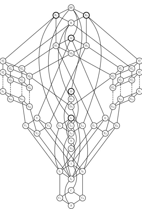
Theorem 2.7 ([Pos41]). 1. The complete list of closed classes of Boolean func- tions is:

– BF, R₀, R₁, R =def R₀ ∩R₁,

– M, M0 =def M∩R0, M1 =def M∩R1, M2 =def M∩R, – D, D₁ =def D∩R, D₂ =def D∩M,

– L, L₀ =def L∩R₀, L₁ =def L∩R₁, L₂ =def L∩R, L₃ =def L∩D, – S0, S02 =def S0∩R, S01=def S0∩M, S00=def S0 ∩R∩M, – S₁, S₁₂ =def S₁∩R, S₁₁=def S₁∩M, S₁₀=def S₁ ∩R∩M,

– S^m₀ , S^m₀₂ =def S^m₀ ∩R, S^m₀₁ =def S^m₀ ∩M, S^m₀₀ =def S^m₀ ∩R∩M for m ≥2, – S^m₁ , S^m₁₂ =def S^m₁ ∩R, S^m₁₁ =def S^m₁ ∩M, S^m₁₀ =def S^m₁ ∩R∩M for m ≥2, – E =def [et]∪[0]∪[1], E₀ =def [et]∪[0], E₁ =def [et]∪[1], E₂ =def [et], – V =def [vel]∪[0]∪[1], V₀ =def [vel]∪[0], V₁ =def [vel]∪[1], V₂ =def [vel], – N =def [non]∪[0], N2 =def [non],

– I =def [id]∪[0]∪[1], I₀ =def [id]∪[0], I₁ =def [id]∪[1], I₂ =def [id], – C =def [0]∪[1], C₀ =def [0], C₁ =def [1] and ∅.

2. All inclusional relationships between the closed classes of Boolean functions are presented in Figure 2.2.

3. There exists an algorithm which, given a finite set B ⊆ BF, determines the closed class of Boolean functions from the list above which coincides with [B].

4. There exists an algorithm which, given f ∈ BF and a finite set B ⊆ BF, decides whether f ∈[B] or not.

Now let us consider two examples:

(24)

R1 R0

BF

R

M

M1 M0

M2

S²0

S³₀

S0

S²₀₂

S³₀₂

S02

S²₀₁

S³₀₁

S01

S²₀₀

S³₀₀

S00

S²1

S³₁

S1

S²₁₂

S³₁₂

S12

S²₁₁

S³₁₁

S11

S²₁₀

S³₁₀

S10

D D1

D2

L

L1 L0

L2

L3

V

V1 V0

V2

E E0

E1

E2

I

I1 I0

I2

N2

C

C1 C0

N

∅

Fig. 2.2.Graph of all classes of Boolean functions being closed under superposition.

(25)

2.2 Boolean functions and closed classes 25

Example 2.8. We define the Boolean function f³ such that f(x, y, z) = 1 iff exactly one argument has the value 1. Clearly, f is 0-reproducing but not 1- reproducing. Now assume that f is a linear function, i.e.,f(x, y, z) =a₀⊕(a₁∧ x)⊕(a₂∧y)⊕(a₃∧z) for suitablea₀, a₁, a₂, a₃ ∈ {0,1}. Sincef(0,0,0) = 0 we know a0 = 0 and it follows that a1 =a2 =a3 = 1, because of f(1,0,0) = f(0,1,0) = f(0,0,1) = 1. But this is a contradiction because f(1,1,1) = 0, showing that f is not linear. Furthermore f is not monotone sincef(1,0,0) = 1 and f(1,1,1) = 0, and it is not self-dual because of f(0,0,0) = f(1,1,1). Finally, f cannot be 1- separating of degree 2 because of f(0,0,1) = f(0,1,0) = 1. Summarizing the above,f is not in R₁, L, M, D, and S²₁ but it is in R₀. A short look at Figure 2.2 shows [{f}] = R0.

Example 2.9. Set B =def {vel, g}, whereg(x, y) = non(aut(x, y)). Now we want to determine [B]. Clearly B is not in R₀, since g(0,0) = 1, but in R₁, because g(1,1) = vel(1,1) = 1. The set B is not linear, because vel is not linear. For this suppose that vel is linear and therefore vel(x, y) = a₀ ⊕(a₁∧x)⊕(a₂∧y), where a₀, a₁, a₂ ∈ {0,1}. Hence a₀ = 0 and a₁ =a₂ = 1, because of vel(0,0) = 0 and vel(0,1) = vel(1,0) = 1. But this is a contradiction, since vel(1,1) = 1 too.

AlsoB is not monotone, since (0,0)<(1,0), butg(0,0) = 1 and g(1,0) = 0 and not selfdual, because vel(0,1) = vel(1,0). Moreover B is not S²₀, since g⁻¹(0) = {(0,1),(1,0)}. By Figure 2.2 we obtain that [B] = R₁.

Because of Theorem 2.7 there exist five maximal non-complete closed classes of Boolean functions, which are circled bold in Figure 2.2. Using these classes the well-known result follows:

Corollary 2.10. A class B of Boolean functions is complete if and only if B 6⊆

R₀, B 6⊆R₁, B 6⊆L, B 6⊆D, and B 6⊆M.

The following theorem gives us some information about bases of closed classes of Boolean functions.

Theorem 2.11 ([Pos41]). Every closed class of Boolean functions has a finite base. In particular:

1. {et,vel,non} is a base of BF.

2. {vel, x∧(y⊕z⊕1)}

is a base of R.

3. {et,aut} is a base of R₀.

4. {vel, x⊕y⊕1} is a base of R₁. 5. {et,vel,0,1} is a base of M.

6. {et,vel,1} is a base of M1. 7. {et,vel,0} is a base of M₀. 8. {et,vel} is a base of M₂. 9. {(x∧y)∨(x∧z)∨(y∧z)}

is a base of D.

10. {(x∧y)∨(x∧z)∨(y∧z)}

is a base of D1.

11. {(x∧y)∨(y∧z)∨(x∧z)}

is a base of D₂.

12. {aut,1} is a base of L.

13. {aut} is a base of L₀. 14. {x⊕y⊕1} is a base of L₁. 15. {x⊕y⊕z} is a base of L₂. 16. {x⊕y⊕z⊕1} is a base of L3. 17. {x∨y} is a base of S₀.

18. {x∧y} is a base of S₁.

(26)

19. {x∨(y∧z)} is a base of S₀₂. 20. {x∧(y∨z)} is a base of S12. 21. {x∨(y∧z)} is a base of S₀₀. 22. {x∧(y∨z)} is a base of S₁₀. 23. {0, x∧(y∨z)} is a base of S11. 24. {1, x∨(y∧z)} is a base of S₀₁. 25. {x∨y,dual(h_m)} is a base of S^m₀ . 26. {x∧y, hm} is a base of S^m₁ . 27. {x∨(y∧z),dual(h_m)}

is a base of S^m₀₂.

28. {x∧(y∨z), hm} is a base of S^m₁₂. 29. {x∨(y∧z),dual(h₂)}

is a base of S²₀₀.

30. {dual(h_m)} is a base of S^m₀₀, where m≥3.

31. {x∧(y∨z), h₂} is a base of S²₁₀. 32. {h_m} is a base of S^m₁₀,

where m≥3.

33. {1,dual(h_m)} is a base of S^m₀₁.

34. {0, h_m} is a base of S^m₁₁. 35. {et,0,1} is a base of E.

36. {et,1} is a base of E₁. 37. {et,0} is a base of E₀. 38. {et} is a base of E2. 39. {vel,0,1} is a base of V.

40. {vel,1} is a base of V₁. 41. {vel,0} is a base of V0. 42. {vel} is a base of V₂. 43. {non,1} is a base of N.

44. {non} is a base of N2. 45. {id,0,1} is a base of I.

46. {id,1} is a base of I₁. 47. {id,0} is a base of I₀. 48. {id} is a base of I₂. 49. {0,1} is a base of C.

50. {1} is a base of C₁. 51. {0} is a base of C₀.

We define hm(x1, . . . , xm+1) =def

m+1W

i=1

(x1∧ · · · ∧xi−1∧xi+1∧ · · · ∧xm+1).

For an n-ary Boolean function f define the Boolean function dual(f) by dual(f)(x₁, . . . , x_n) =def f(x₁, . . . , x_n). The functions f and dual(f) are said to be dual. Obviously, dual(dual(f)) = f. Furthermore, f is self-dual iff dual(f) = f.

For a class F of Boolean functions define dual(F) =def {dual(f) | f ∈ F}. The classes F and dual(F) are called dual.

For some examples of Boolean functions and their dual function see Figure 2.3.

f dual(f) 0 1 1 0 et(x, y) vel(x, y) vel(x, y) et(x, y)

non(x) non(x) id(x) id(x) aut(x, y) aeq(x, y) et(x,non(y)) vel(x,non(y)) Fig. 2.3.Some Boolean functions and their dual function.

Proposition 2.12 (Duality principle). 1. Let g be a Boolean function such thatg(x₁, . . . , x_n) =f(f₁(x¹₁, . . . , x¹_m₁), . . . , f_l(x^l₁, . . . , x^l_m_l)). For the dual func- tion of g it holds that dual(g) = dual(f)(dual(f₁), . . . ,dual(f_l)).

2. If B is a finite set of Boolean functions then [dual(B)] = dual([B]).

(27)

2.3 Generalized circuits and formulas 27

3. Every closed class is dual to its “mirror class” (via the symmetry axis in Figure 2.2).

4. Let F be a closed class. Then dual(F) is a closed class too.

Proof. For the first statement observe the following:

dual(g) = dual(f(f₁(x¹₁, . . . , x¹_m₁), . . . , f_l(x^l₁, . . . , x^l_m_l)))

=¬f(f₁(¬x¹₁, . . . ,¬x¹_m₁), . . . , f_l(¬x^l₁, . . . ,¬x^l_m_l))

=¬f(¬¬f1(¬x¹₁, . . . ,¬x¹_m₁), . . . ,¬¬fl(¬x^l₁, . . . ,¬x^l_m_l))

=¬f(¬dual(f₁(x¹₁, . . . , x¹_m₁)), . . . ,¬dual(f_l(x^l₁, . . . , x^l_m_l)))

= dual(f)(dual(f₁(x¹₁, . . . , x¹_m₁)), . . . ,dual(f_l(x^l₁, . . . , x^l_m_l))) The second statement is a direct consequence of the first statement.

For the third statement use the base B of an arbitrary closed class, given by Theorem 2.11, and calculate dual(B). Again by Theorem 2.11 we obtain that dual(B) is a base of the “mirror class”, which proves the claim by the second statement.

Finally note that the last statement is also a direct consequence of the second

statement. ut

2.3 Generalized circuits and formulas

In the present work we focus on the study of computational problems related to generalized circuits and formulas, which are closely related to Post’s framework (cf. Section 2.2). Hence we will introduce them in this section.

In basic textbooks propositional logic is always introduced in two steps. First we define the syntax by specifying propositional variables and connectors for combining them and the second step is the definition of the semantic of the defined formulas. In this step we associate a Boolean function to each connector.

It is common to use ∧, ∨ and ¬ as symbols for the Boolean functions et, vel and non, because {et,vel,non} is a complete set (cf. Corollary 2.10), and thus we can represent all Boolean functions by using formulas, which are build by making use of ∧, ∨ and ¬ as connectors for propositional variables. A natural generalization would be the following approach. Choose a finite set of Boolean functions, not necessarily complete, and symbols for them. Now define formulas by using these symbols as connectors and their corresponding Boolean function as the semantic of them. By doing so, we can introduce for each fixed setB another generalized propositional logic. In a similar way we can introduce circuits. Here we only use gate-types which represent Boolean functions out of the fixed set of Boolean functions to build our circuits.

In the following chapters we will study various problems related to such generalized circuits and formulas, but due to the overwhelming number of them we have to restrict ourselves to a special subset of these problems. To have an easy to use definition we will first introduce our generalized circuits and after that we will consider the generalized formulas as a special case of them.