Effects of inflation expectations on macroeconomic dynamics:
extrapolative versus regressive expectations
Marji Lines and Frank Westerhoff
Working Paper No. 68 December 2009
k*
b
0 k
B A M
AMBERG CONOMIC
ESEARCH ROUP
B E R G
Working Paper Series BERG
on Government and Growth
Bamberg Economic Research Group on Government and Growth
Bamberg University Feldkirchenstraße 21
D-96045 Bamberg Telefax: (0951) 863 5547 Telephone: (0951) 863 2547 E-mail: public-finance@uni-bamberg.de http://www.uni-bamberg.de/vwl-fiwi/forschung/berg/
ISBN 978-3-931052-76-8
Reihenherausgeber: BERG Heinz-Dieter Wenzel Redaktion
Felix Stübben ∗
Effects of inflation expectations on macroeconomic dynamics:
extrapolative versus regressive expectations
Marji Lines
aand Frank Westerhoff
ba
Department of Statistics, University of Udine, Via Treppo 18, 33100 Udine, Italy Email: lines@dss.uniud.it
b
Department of Economics, University of Bamberg, Feldkirchenstrasse 21, 96045 Bamberg, Germany Email: frank.westerhoff@uni-bamberg.de
Abstract
In this paper we integrate heterogeneous inflation expectations into a simple monetary model. Guided by empirical evidence we assume that boundedly rational agents, selecting between extrapolative and regressive forecasting rules to predict the future inflation rate, prefer rules that have produced low prediction errors in the past. We show that integrating this behavioral expectation formation process into the monetary model leads to the possibility of endogenous macroeconomic dynamics. For instance, our model replicates certain empirical regularities such as irregular growth cycles or inflation persistence.
Moreover, we observe multi-stability via a Chenciner bifurcation.
Keywords
Extrapolative and regressive expectations; dynamic predictor selection; macroeconomic dynamics; nonlinearities and chaos; bifurcation analysis.
JEL classification
C62; C63; E31; E32.
1 Introduction
Many macroeconomic models restrict their attention to the behavior of a representative agent which, when it comes to the formation of expectations, relies on a single strategy to forecast macroeconomic variables. For some time this strategy was given by an extrapolative, adaptive or regressive prediction rule but after the late 1970s rational expectations became the leading paradigm. However, empirical evidence makes it obvious that views about future economic variables may differ considerably among economic agents. A study by Mankiw et al. (2003), who analyze survey data on inflation expectations, illustrates this aspect quite clearly. Their data set reveals that the interquartile range of inflation expectations for 2003 among economists ranges from 1.5 to 2.5 percent and that among the general public, the interquartile range of expected inflation ranges between 0 and 5 percent. Similar results are reported, for instance, by Carroll (2003) and Pesaran and Weale (2006). It seems that inflation expectations are neither consistent with the notion of a fully rational behavior nor by the representative agent assumption.
An important question for macroeconomic theory thus is how agents form
expectations in reality. First of all, a number of empirical papers (Simon 1955, Kahneman,
Slovic and Tversky 1986, Smith 1991) indicate that people should be regarded as
boundedly rational and that they display in many situations a rule-governed behavior. In
particular, people seem to rely on a limited number of heuristic principles which have
proven to be useful in the past. Further empirical evidence by Hommes et al. (2005) and
Heemeijer et al. (2009) even tells us that agents use rather simple linear forecasting rules
to form predictions. For instance, agents used extrapolative and regressive expectation
formation rules in their experiments. Also Branch (2004) finds from the analysis of survey
data on inflation expectations that agents rely on heuristic forecasting principles.
Interestingly, agents do not hold on to a particular rule but select rules which have generated low prediction errors in the past. The choice of a predictor may furthermore be biased by a predisposition effect, i.e. a behavioral preference for a certain type of rule.
More empirical evidence on heterogeneous expectations and dynamic predictor selection in different economic contexts is provided by Chavas (2000), Alfarano et al. (2005), Boswijk et al. (2007) and Goldbaum and Mizrach (2008), Lux (2009), among others.
The main goal of this paper is to improve our understanding about the relation between heterogeneous inflation expectations and macroeconomic dynamics. We use a well-known monetary model as a workhorse and try to ground our modeling of heterogeneous inflation expectations on empirical observations. The basic structure of our model is as follows. We use Okun’s law and the expectations-augmented Phillips curve to describe the supply side of the economy. In addition, we employ an aggregate demand relation in which output growth is driven by both changes in nominal money growth and inflation. Of key importance is how we treat the agents’ expectation formation process.
Guided by empirical evidence, agents select between competing forecasting strategies based on an evolutionary fitness measure. To be precise, we assume that the agents prefer predictors with a high forecasting accuracy, measured in terms of squared forecasting errors. Moreover, agents either form extrapolative expectations, that is, they believe that the current inflation trend will continue, or they form regressive expectations, that is, they guess that the inflation rate will return towards its normal value.
Analytical and numerical investigations reveal that our four-dimensional nonlinear
deterministic model has the potential to generate complex macroeconomic dynamics and
thus provides intuitions on how irregular inflation, growth and unemployment cycles
might emerge in real economies. The main economic reason is that there prevails, for a
broad range of parameter combinations, a permanent evolutionary competition between
stabilizing and destabilizing prediction rules. Suppose that the majority of agents rely on the regressive predictor. Then the dynamics is stable and a convergence towards a
“normal” steady state sets in. However, the system does not necessarily settle down on this fixed point. Close to the steady state the forecasting accuracies of both predictors become similar. If a sufficient number of agents switch to the extrapolative predictor, the steady state becomes unstable and oscillations in key macroeconomic variables are triggered. Regressive expectations may gain in popularity again when the prediction errors of extrapolative expectations become strong. The dynamics get complicated due to further macroeconomic feedback processes.
Another interesting finding is that part of the parameter space is characterized by multi-stability, a phenomenon with important consequences for macroeconomic policy design. Numerical simulations suggest that a locally stable steady state coexists with locally stable limit sets on closed curves or even chaotic attractors. As a result, the model variables are driven towards the steady state for some initial conditions and remain there as long as exogenous shocks are not too large. However, significant exogenous disturbances may kick the economy out of the steady state’s basin of attraction, and only another kick (e.g. performed via monetary or fiscal policies) will get the economy back into that basin. Otherwise, the economy is destined to some sort of “endogenous”
fluctuation, even though an equilibrium exists and is locally stable. Macroeconomic policy interventions, if they are well designed, may keep the system close to the steady state.
Our paper is closely related to Lines and Westerhoff (2009) where we also use a
monetary model as a starting point for their analysis but concentrate on the case of
rational and extrapolative expectations. One result of that paper is that macroeconomic
dynamics may be subject to a phenomenon called intermittency, i.e. the inflation rate may
stay very close to its normal value for an extended period of time, but then, apparently out of the blue, wild inflation rate changes emerge. Numerical studies of the model presented in this paper suggest that the dynamics have a stronger cyclical nature which seems to be more consistent with real macroeconomic dynamics. Moreover, rational expectations can only be regarded as a theoretical benchmark scenario since there is no empirical evidence for such behavior in real data. The object of this paper is to work with forecasting rules which are empirically observable.
Note that there are several other interesting papers in this area and we mention a few of them here. For instance, Branch and McGough (2008, 2009) investigate the role of heterogeneous expectation formation within a New Keynesian framework. In their model, agents have to predict both the future inflation rate and the future output level. Franke (2007) also considers a model in which agents use different forecasting rules to predict the inflation rate. An interesting insight of his paper is that the average of these inflation forecasts may be interpreted as a proxy for the current inflation climate (which circumvents a more or less open aggregation problem to which we come back later). The papers by Anufriev et al. (2008) and de Grauwe (2008) explore how monetary policy rules may work in such approaches. Westerhoff (2006) does the same but with a focus on the effectiveness of some common fiscal policy rules. Some contributions stress the agents’
learning behavior more strongly. For instance, Berardi (2007) considers a model which is populated by two different types of agents who learn through recursive least squares techniques the parameter values of their forecasting strategies. Tuinstra and Wagener (2006) come up with an interesting setup which includes an evolutionary competition between two different estimation procedures.
This brief survey illustrates the extent to which heterogeneous expectations have
come to matter in explanations of the behavior of macroeconomic variables. We hope that
the present paper adds to this interesting and relevant stream of literature. From a broader point of view, our work is directly related to the theory of nonlinear macroeconomic dynamics as developed and surveyed by, among others, Day (1999), Rosser (2000), Puu and Sushko (2006) and Chiarella et al. (2005, 2009).
The remainder of the paper is organized as follows. In section 2, we present our model and discuss some properties of its dynamical system, including the local stability of the model’s unique fixed point. In Section 3, we determine a basic parameter setting via a rough calibration of the model and discuss the functioning of our approach. In Section 4, we check the robustness of our findings and point out some interesting dynamical features of our model. Finally, Section 5 concludes the paper.
2 A monetary model with heterogeneous expectations
In this section, we develop a monetary model with heterogeneous expectations. Our model
comprises four building blocks. The first three building blocks, i.e. Okun’s law, an
expectations-augmented Phillips curve and an aggregate demand relation, constitute the
macroeconomic environment of the model (see, for instance, Blanchard 2009). The novel
feature of our model is the forth building block which describes how agents form inflation
expectations. As in the predictor choice framework of Brock and Hommes (1997, 1998),
agents select between different types of forecasting rules with respect to the rules past
performance. Note that agents display a boundedly rational learning behavior in the sense
that they tend to select forecasting rules which have produced low forecasting errors in the
recent past. At the end of this section, we show that the dynamics of our model is due to a
four-dimensional nonlinear dynamical system. As it turns out, the model has a unique
steady state and we are able to determine its (local) stability properties (mathematical
details are presented in the Appendix).
We begin with Okun’s law, according to which, a change in the unemployment rate from period t to period t-1 can be explained by the current deviation of the output growth rate from its normal value . Okun’s law, which is empirically supported and mainly driven by (labor) productivity growth, may be expressed as
u t
g t g n
)
1 ( t n
t
t u g g
u − − = − β − , (1) where β is a positive parameter. Notice that output growth above normal leads to a decrease in the unemployment rate. To maintain a stable unemployment rate, output growth obviously must be equal to the normal output growth. The unemployment rate increases if output growth drops below normal output growth.
Within the expectations-augmented Phillips curve, the inflation rate π t depends on the expected inflation rate and on the deviation of the unemployment rate from its natural rate . A standard formulation is
t e
π
u n
) ( t n
t e
t π α u u
π = − − , (2) where is a positive parameter. The intuition of (2) is as follows. First, workers expecting a high inflation rate will request a wage raise. Mark up pricing of firms then increases the inflation rate. Second, if the unemployment rate decreases, workers have a stronger bargaining power and are able to negotiate higher wages. Mark up pricing of the firms again drives the inflation rate upwards.
α
We apply a standard aggregate demand relation in which the output growth rate depends on the difference between nominal money growth and the inflation rate. Since we assume that the nominal money growth rate is constant over time, we obtain for the output growth rate
m
t
t m π
g = − . (3)
As is well-known, (3) is consistent with the classical IS-LM framework. The argument is as follows. If money growth exceeds inflation, the real money stock increases. As a result, the interest rate decreases which, in turn, stimulates the demand for goods. Hence, output also increases.
The three building blocks of this monetary model have some important implications which we briefly mention here. Note first that by combining (1)-(3) it is possible to write
αβ π π αβ π αβ
g m
π t αβ n t t e t e
+ + − + +
+
= − − −
1 1
1
)
( 1 1
, (4) i.e. the inflation rate in period t depends on the inflation rate in period t-1 and on the expected inflation rates in periods t and t-1. Let π stand for the equilibrium inflation rate.
Then, (4) implies that
) (
)
( m − g n + t e − t e − 1
= αβ π π
π . (5) Moreover, if there are no further changes in expectations we obtain from (5) that the equilibrium inflation rate is given by the distance between the (constant) money growth rate and the normal output growth rate. The equilibrium inflation rate is also called the normal inflation rate π n and formally given by
n n = π = m − g
π . (6) It is reasonable to assume in the following that the agents expect the inflation rate correctly in equilibrium. Doing this, we have that the steady state unemployment rate is equal to the natural unemployment rate (via the Phillips curve) and that the steady state output growth rate is equal to the normal output growth rate (via Okun’s law).
Let us now turn to the last and decisive building block of our model, the
expectation formation behavior of heterogeneous boundedly rational agents. As indicated
in the introduction, empirical evidence suggests that agents apply different strategies to forecast the inflation rate. This is exactly what happens in our model. Agents select between competing prediction strategies on the basis the strategies’ squared prediction errors which means they are characterized by boundedly rational learning behavior. We concentrate on two competing prediction rules: a simple and cheap extrapolative predictor and a more sophisticated but costly regressive predictor. The average expected value of the inflation rate thus is defined as
t R t R t E t E
t e w π w π
π = + , (7) where is the relative weight of extrapolative expectations and is the relative weight of regressive expectations , respectively.
t E
w π t E w t R
t R
π
1Agents forecast the inflation rate for period t conditional on the information set available at period t-1. Simple extrapolative expectations may be expressed as
)
( 1 2
1 − −
− + −
= t t t
t E π γ π π
π , (8) where γ > 0 indicates how strong the agents extrapolate past inflation trends into the future. Regressive expectations, in turn, are usually formalized as
)
( 1
1 −
− + −
= t n t
t R π δ π π
π . (9) Hence, the agents expect that the inflation rate will return towards its normal value over time. The expected adjustment speed depends on 0 < δ < 1 .
The agents do not stick to a certain rule but compare their relative performance.
We assume that the agents prefer heuristics with a high forecasting accuracy and rely on
1
Note that we include heterogeneous expectations in form of a weighted average of individual expectations
into an otherwise linear macroeconomic model which has no explicit microfoundation. Although Anufriev
et al. (2008) conclude that this is the most natural way to do, it is clear that this aggregation aspect deserves
more attention in the future.
squared prediction errors as a (publicly observable) fitness measure. The attractiveness of extrapolative expectations is defined as
1 2
1 )
( − − −
−
= t E t
t E
a π π , (10) while the attractiveness of the regressive expectation is given as
κ π
π − −
−
= ( t R − 1 t − 1 ) 2
t R
a . (11) Note first that forming regressive expectations may in fact be costly since one has to develop some kind of general knowledge about the working of the economy. In particular, the agents have to consider what is the normal inflation rate and how quickly does the actual inflation rate converge towards that value. Moreover, agents may have a behavioral bias for a certain type of predictor. In our model agents have a preference/predisposition for simple extrapolative rules. The term κ ≥ 0 in (11) captures both aspects (note the negative sign in front of κ which reduces the fitness of regressive expectations).
As in Brock and Hommes (1997, 1998), we update the fractions of agents using the one or the other predictor via a discrete-choice model. The weights of the two predictors are given as
] [ ]
[
] [
t R t E
t E t E
a Exp a
Exp
a w Exp
λ λ
λ
= + (12) and
] [ ] [
] [
t R t E
t R t R
a Exp a
Exp
a w Exp
λ λ
λ
= + . (13)
Parameter λ ≥ 0 is called the intensity of choice since it describes how sensitive the mass
of agents is to selecting the most attractive predictor. Loosely speaking, an increase in λ
may be regarded as an increase in the (bounded) rationality of the agents. To see this note
first that for λ = 0 , half of the agents relies on the extrapolative predictor and the other
half on the regressive predictor, i.e. they do not discriminate between differently performing predictors. As λ increase, however, more and more agents select the predictor with the higher fitness. In the extreme case in which λ goes to plus infinity, all agents select the best performing predictor.
Inserting (7)-(13) into (4) gives the evolution of the inflation rate as a fourth-order nonlinear difference equation, that is
) , , ,
( − 1 − 2 − 3 − 4
= t t t t
t f π π π π
π . (14) Auxiliary variables can be introduced and (14) can be written and simulated as a four- dimensional first-order system. Fortunately, the Jacobian matrix and the characteristic equation can be written explicitly for the unique fixed point, so that local stability of π n can be directly determined. Using the coefficients of the resulting third-degree polynomial (one eigenvalue is always zero), the relevant inequalities associated with loss of hyperbolicity and specific bifurcations suggest that the only loss of local stability is through the modulus of a pair of complex conjugate eigenvalues crossing the unit circle, that is, the Neimark-Sacker (henceforth N-S) bifurcations. Our analytical results are summarized in the following proposition.
Proposition: The monetary model (1)-(3), expanded to include heterogeneous expectations and a dynamic predictor selection (7)-(13), has a unique steady state in which the inflation rate, the unemployment rate and the output growth rate correspond to their natural values. Moreover, the steady state of the underlying four-dimensional nonlinear dynamical system loses stability through a Neimark-Sacker bifurcation for a given constellation of parameter values. In terms of the extrapolation parameter the critical value is
)) 1 ( 2 ) 1 ( (
) 1 ( 1
− +
−
− +
= −
i i
i
i
c μ i δ μ
μ
γ δ , setting = + αβ
1
i 1 and μ − λκ
= + e 1
1 . (15)
Proof of the Proposition is given in the mathematical appendix, where the stability conditions of the steady state are given. It is possible to then determine how specific parameters influence the inequality condition associated with the N-S bifurcation. The higher the extrapolation coefficient γ the closer the stability inequality is to zero, that is, to the critical value of the bifurcation. The effects of the other parameters are not uniquely determined. For the relevant part of parameter space, however, we have the following relations. The higher the regressive predictor coefficient δ the larger the parameter subspace leading to local steady state stability. The selection criterion parameters λ and κ are inversely related to the inequality condition, that is, more sensitivity to performance or higher costs for the regressive predictor lead to a smaller subspace of local stability for the steady state. The monetary model parameters, α and β , are directly related to the inequality, so that increasing either the sensitivity of the inflation rate to distance from normal unemployment rate or that of unemployment changes to distance from normal output growth rate will shrink the parameter subspace of local stability. All of these results make sense and all are confirmed in numerical simulations.
We were not able to determine the condition that would permit us to state the
stability of the curves emerging from the N-S bifurcation. Numerical exercises indicate
that the N-S bifurcation is of subcritical type so that in a sufficiently small left
neighborhood of γ c the curves bifurcating from (and enclosing) π n are repelling. That is,
the invariant curves appearing before the critical parameter value form a boundary for the
basin of attraction of the steady state inflation rate. This situation is called “corridor
stability” and trajectories starting from initial values falling outside of the closed curve
either explode to infinity or are attracted to some other limit set. The corridor, the basin of
attraction of the equilibrium, decreases until, at the critical parameter value, it disappears altogether.
However, simulations suggest that the global dynamical behavior over much of the relevant parameter space is motion on, or close to, stable closed curves and that part of the parameter space characterized by the coexistence of these limit sets and the stable π n . This combination of analytical results and numerical experiments suggest that the subcritical N-S bifurcation is accompanied by a two-parameter bifurcation known as a Chenciner bifurcation (for economic applications and technical references see Neugart and Tuinstra 2003, Agliari 2006, Agliari et al. 2006, Gaunersdorfer et al. 2008). These intriguing features will be discussed in more detail in Section 4.
3 Calibration and functioning of the model
The aim of this section is to conduct a rough, first-order calibration to obtain an initial, basic parameter setting for our subsequent numerical analysis and discuss the functioning of the model. We focus on calibration in order to ensure that our simple deterministic model has some potential to generate reasonable macroeconomic dynamics. Then, in Section 4, we discuss the robustness of our findings and mention interesting model properties under different sets of parameter values.
In total, there are nine parameters in the model. Five parameters are related to the macroeconomic part of the model while four belong to the expectation formation part of the model. The basic macroeconomic parameter values are
02 . 0
n =
g , u n = 0 . 05 , m = 0 . 05 , α = 1 , β = 0 . 35 ,
i.e. the normal output growth rate is 2 percent, the normal rate of unemployment is 5
percent and the nominal money growth is 5 percent, which seem to be reasonable values.
Note that the slope parameters of the Phillips curve and Okun’s law are in line with empirical observations (they are taken from Blanchard 2009) and the same as in the companion paper of Lines and Westerhoff (2009).
We experimented extensively with the expectation related parameters and finally chose this representative set of values:
95 . 0
γ = , δ = 0 . 5 , κ = 0 . 0001 and λ = 30000 .
Accordingly, agents either believe that 95 percent of the current inflation trend will persist or expect a mean reversion of 50 percent. Prediction costs and behavioral bias towards extrapolative expectations jointly correspond to a one percent squared prediction error.
The impact of parameter λ on the strategy selection behavior of the agents can be understood in conjunction with parameter κ . A value of λ = 30000 for the intensity of choice parameter implies that for our value of κ we have about 95 percent of the agents relying on extrapolative expectations when the squared prediction errors of both strategies are identical (as, e.g., in the steady state). Of course, if the squared prediction error of the extrapolative rule is 0.0001 units larger than the squared prediction error of the regressive rule (say, the actual inflation rate is 1 percent, the extrapolative prediction is 3 percent and the regressive prediction is 2.733 percent) the weights of both strategies are equal to 50 percent. Finally, a 0.0002 units larger squared prediction error of the extrapolative rule versus the regressive rule implies a reduction in the weight of extrapolators to about 5 percent.
All in all, our assumptions about κ and λ imply that agents prefer extrapolative
rules over regressive rules. For a turn-around from 95 percent extrapolators to 5 percent
extrapolators the rules’ squared prediction error differential has to be 0.0002 units. At first
sight, a value of 30000 for λ may seem high but we think that the examples illustrate that
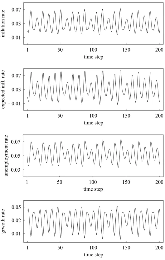
We now turn to an exploration of the dynamics of the model. In Figure 1, the panels display from top to bottom the evolution of the inflation rate, the expected inflation rate, the unemployment rate and the output growth rate. We observe, for instance, irregular growth cycles with varying amplitudes. Similar, there are periods where changes in the unemployment rate are rather low, followed by some larger swings. Note also that output and unemployment fluctuate countercyclical. A reduction in growth rates drives the unemployment rate up (and vive versa), as we would expect in reality. Since the forecasting errors are obviously not dramatic (the correlation coefficient is 0.92) the agents’ behavior should not be regarded as irrational.
PLACE FIGURE 1 ABOUT HERE
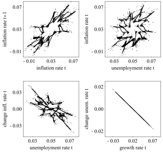
In Figure 2 we look at the behavior of, and relations between, economic variables.
The top left panel shows the inflation rate in period t+1 versus the inflation rate in period t. As in actual economies there is clear evidence for persistence of inflation: if inflation is high (low) in period t, it is quite likely that inflation will also be high (low) in period t+1.
Next, the panel in the top right depicts the inflation rate in period t versus the
unemployment rate in period t. Interestingly, the “original” Phillips curve does not appear
in our artificial data, as is the case for real data since the 1970s. However, there is
evidence of a “modified” (plump) Phillips curve, in the panel at the bottom left, in which a
decrease in the unemployment rate leads to an acceleration of the inflation rate. We find it
quite remarkable that our simple deterministic model may jointly generate these two
important and much debated stylized facts. Finally, in Figure 2, bottom right, the
simulated data points follow Okun’s law. Overall, our model seems to be able to replicate
some prominent empirical relations between key macroeconomic variables and we may
thus conclude that our basic parameter setting appears to be reasonable, at least at first
sight.
PLACE FIGURE 2 ABOUT HERE
Let us next try to understand how the model works. Consider the beginning of an upturn. At the steady state, both predictors are perfect, but because reversion predictors have associated costs, the majority of the agents relies on extrapolative expectations. As the inflation rate starts to deviate from equilibrium, errors of regressive expectations start to exceed those of extrapolative expectations and agents prefer the cheaper predictor even more. There follows an exponential expansion as more agents switch to extrapolation, increasing its weight in the aggregate expectation which gives a higher inflation rate. The switching is exasperated by larger errors for reversion expectations as the inflation rate moves further away from the steady state inflation rate.
Near the end of the expansion phase most agents are trend-followers. On the one hand, with movement to extrapolation having fallen off, the push on the inflation rate through the aggregate expectation slows. On the other hand, a few agents still use the reversion predictor and their expectation is that of a heavy turn-around. These two effects work through the aggregate expectation to slow the expansion. Moreover, at some distance from equilibrium, a stabilizing macroeconomic feedback kicks in. As the inflation rate increases, real money growth declines which, in turn, reduces aggregate demand (via the aggregate demand relation). The reduction in output increases the unemployment rate (via Okun’s law). Since this decreases the wage pressure, inflation declines (via the Phillips curve).
At the turning point extrapolation produces larger errors and agents begin to
switch back to the reversion expectation. Once the turning point is past, the direction of
motion changes, and in the return to equilibrium, extrapolative and reversion predictors
are heading in the same direction. The result is a quick return to the vicinity of the steady
state inflation rate. Near this value both predictors make small errors but the sophisticated
predictor costs. Extrapolators outnumber agents using the reversion predictor and the trend continues downward, past the equilibrium, with the same dynamics described above, a phase of decline followed by a turn-around.
This long run fluctuating behavior may be characterized by periodic, quasiperiodic or chaotic motion and we next use further numerical methods to explore the sensitivity of the dynamics with respect to the various parameters introduced through the heterogeneous expectations framework.
4 Sensitivity analysis and dynamic properties of the model
Now we explore how the model parameters related to the expectation formation behavior of the agents impact on the dynamics. For this task we make use of a powerful numerical tool that allows a pairwise analysis of parameters, namely two-dimensional bifurcation diagrams. In particular, we compare parameters κ versus λ (figure 3), γ versus δ (figure 4), and γ versus λ (figure 5). These numerical exercises are indispensable for understanding the role played by parameters. We finally also illustrate the phenomenon of bistability found in the Chenciner bifurcation (figures 5 to 7).
Consider first the two parameters characterizing the dynamic predictor selection part of the model: κ , the actual and behavioral costs involved in forming regressive expectations, and λ , the agents sensitivity to performance differentials. In Figure 3, limit sets are represented over parameter space ( κ , λ ) with the standard set of values, but
) 0002 . 0 , 0 (
κ ∈ and λ ∈ ( 0 , 60000 ) , that is, from zero to twice the standard values.
2PLACE FIGURE 3 ABOUT HERE
2
Figures 3 to 7 are produced with the open-source software iDMC which is available at
http://code.google.com/p/idmc/, along with the model system used in this paper.
In double bifurcation diagrams a trajectory is generated for every coordinate couple of parameter values and the long-run dynamics associated with that couple is designated by a color (using the standard set of other parameter values, and from a given initial point). If asymptotic dynamics are a stable fixed point, the coordinate is colored red (gray area in southwest corner). The other colored areas represent parameter combinations for which stable cycles composed of the indicated number of periodic points exist. The white area represents combinations for which the dynamics are either: periodic but of period higher than the maximum cycle sought; quasiperiodic (and like periodic cycles the sequences lie on an invariant curve); chaotic (and points lie on a strange attractor). A black area represents combinations for which the trajectories tend to infinity.
Figure 3 suggests a sensitive dependency on parameter values, that is, nearby parameter values can give rise to completely different types of long-run dynamics. In general, for small values of both parameters, the inflation rate is stable, but even if costs are very low, endogenous fluctuations may result if agents are very sensitive to performance. There appears to be a smooth boundary between fixed point and fluctuating long-run dynamics, except for what appears to be a quasiperiodic island occurring in the fixed point zone. The island suggests that multi-stability exists even for low costs and/or weak predisposition effects and that initial conditions will determine the limit set to which the trajectory is eventually attracted. It should be noted that, under the standard set of values, neither high κ nor high λ ever cause the system to lose stability.
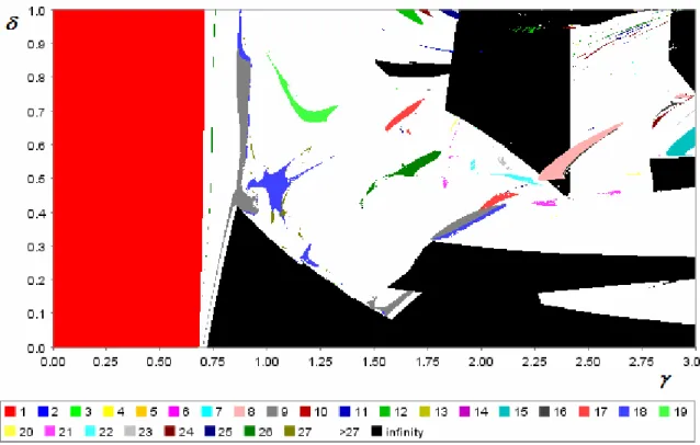
Consider next Figure 4, with the standard set of values except γ ∈ ( 0 , 3 ) and )
1 , 0 (
δ ∈ (the full hypothesized range for δ ). The essential role of the extrapolation
parameter is clear. In order that the equilibrium inflation rate attracts trajectories from the
given initial value, γ must be smaller than a threshold value. For this constellation of
parameters and initial values the threshold appears to be around 0.68. However, the critical value of the N-S bifurcation (15), at which the equilibrium value loses local stability, is larger, γ c = 0 . 732 . Apparently there is again multi-stability for some parts of this parameter space and another limit set attracts trajectories beginning at sufficient distance from the normal inflation rate, even if the critical value of γ has not been reached. Above the threshold value asymptotic dynamics are characterized by quasiperiodic, periodic or chaotic dynamics.
PLACE FIGURE 4 ABOUT HERE
The regression expectation parameter δ , appears to influence dynamics only once the threshold value is crossed and the inflation rate has lost stability. However, there is a positive slope, barely visible in Figure 4 due to the exaggerated interval for γ . Along the slope, as trend followers reach the threshold values for γ , the agents with regressive expectations will counterbalance that destabilization if they believe the return is quick enough ( δ high).
Overall, if the inflation rate is expected to return only slowly to normal ( δ low) and/or trend followers are aggressive ( γ high) the system is more likely to lose all stability (black areas). Even in cases where attractors exist beyond γ = 2 , the inflation rate typically fluctuates wildly and in such an economy some changes in macroeconomic policy would be forthcoming.
Our numerical simulations suggest that of the parameters introduced through the
heterogeneous expectations framework, γ the extent to which trend followers expect the
trend to continue and λ , the switching parameter, are those that most influence the limit
sets to which the economic variables converge. We thus take a closer look at dynamic
scenarios for intervals of these parameters. We begin, in Figure 5 top, with a bifurcation
diagram, representing the limit sets for γ ∈ ( 0 . 65 , 1 . 3 ) and λ ∈ ( 0 , 40000 ) . Again, stable fixed points are in red, on the lower left, colored areas are periodic cycles, the white area represents either high period cycles, quasiperiodic or chaotic motion. Clearly there is sensitive dependency on parameter values.
PLACE FIGURE 5 ABOUT HERE
As in the previous two figures, there are again multiple attractors visible so that initial conditions matter. For example, the curve representing critical parameter values for the N-S (local) bifurcation of the fixed point has been superimposed in black on the plot.
The N-S curve, independent of initial conditions, lies to the right of the curve separating fixed point from non-fixed point dynamical behavior. The latter curve, which we call a fluctuation border, is particular to the given set of parameter values and, importantly, to the given initial value. For instance, take λ constant at 30000, starting from γ = 0 . 68 on the left. The change in limit set represented by the fluctuation border is a global bifurcation. The inflation rate loses stability before reaching the N-S curve which is an indicator of local loss of stability. The fixed point is still stable in the area between the fluctuation border and the N-S curve, but is attracting only for initial conditions within the corridor (see also discussion of Figure 6).
In order to distinguish the limit sets in the white area we make use of plots that indicate the Lyapunov characteristic exponents spectrum over the same parameter space, in Figure 5 bottom. For this model the spectrum is composed of 4 Lyapunov exponents, one for each dimension. Periodic (including period 1) behavior is characterized by 4 negative values; quasiperiodic behavior by the largest exponent zero; chaotic behavior by at least one positive exponent.
Certain general aspects are immediately obvious. The fluctuation border in Figure
5 top appears as the curve that separates parameter combinations leading to limit sets with
a negative spectrum from those leading to 1 zero and 3 negative exponents, that is, the curve separates fixed point dynamics from quasiperiodic dynamics on a closed curve.
Moving further to the right a porous curve separates the area with one zero from that of one positive exponent (the others negative), that is, separates quasiperiodic from chaotic dynamics. To the right of this porous curve (we call it the torus-breakdown border) we see the areas of periodic behavior marked with negative spectra, some of which were visible in Figure 5 top (those with periodicity higher than 32 were not). These periodic islands lie in a sea of chaotic attractors with rare cases of quasiperiodicity.
It should be noted that the presentation of Lyapunov exponents over parameter space requires a definition of zero. The figure changes slightly as the extremes of zero vary. In Figure 5 bottom, zero is defined as 0 ∈ ( − 0 . 005 , 0 . 005 ) . If we loosen the definition, to say 0 ∈ ( − 0 . 01 , 0 . 01 ) , the largest negative or smallest positive Lyapunov exponent may be redefined as a zero. These changes occur, in particular, around the edges of the periodic islands and along the fluctuation and torus-breakdown borders.
It is a common occurrence in nonlinear systems for multiple attractors to exist for the same parameter constellation, and initial values determine to which attractor trajectories converge. Although basins of attraction are in a four-dimensional space, we project the basin of attraction to give an idea of the co-existing basins of attraction.
Consider parameter pairs, in Figure 5, to the left of the N-S critical curve, but to the right of fixed point stability. For these values there are two coexisting equilibrium sets in the state space: a closed curve , on which dynamics are quasiperiodic or periodic; the unique fixed point of the model
Γ s
π n . These are separated by the unstable closed curve of
the N-S bifurcation, the outer boundary of the corridor, call it Γ U , which lies inside of the
larger radius curve Γ s . Only initial conditions lying inside Γ U that is, inside the corridor, converge to π n .
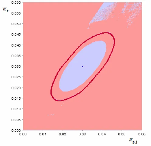
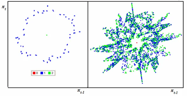
This is the case represented in Figure 6, with γ = 0 . 7 in the state space ( π t − 1 , π t ).
The projection is obtained by letting values of the current and first lag inflation rate vary over (0.00, 0.06), but setting the second and third lags at 0.01. The plot is a two- dimensional slice of the four-dimensional state space. The equilibrium inflation rate basin of attraction is the area immediately around π n . Most of the trajectories starting in the rest of the state space converge to the quasiperiodic attractor on the invariant curve Γ s (burgundy color). The unstable curve Γ U forms the boundary of the basin of attraction of
π n (in blue). It will be observed that there are initial values in the northeast corner that are high for current and first lag inflation rate, yet converge to equilibrium. This is due to having fixed the second and third lag inflation rate values so low.
PLACE FIGURE 6 ABOUT HERE
This basin configuration in the state space has some intriguing dynamical aspects for policy analysis. There exists a neighborhood of the equilibrium value which is attracted to it, while initial value pairs further from equilibrium converge to a curve implying fluctuations. If exogenous disturbances kick the economy out of the basin of π n , only another kick will get the economy back into the equilibrium basin. Otherwise, the economy is destined to some sort of “endogenous” fluctuation, even though an equilibrium exists and is locally stable.
Multi-stability disappears for parameter values beyond the N-S curve. As values
are changed to be closer to the bifurcation, the corridor ring Γ U shrinks until, at the N-S
critical value, it merges with π n , which becomes unstable. That is, once past the N-S
curve the fixed point is unstable and no longer attracts any initial conditions, leaving the only attractor . From an initial value in the state space near Γ s π n , it is observed that the long run dynamics jump from the stable fixed point to a curve which encloses it, as the N- S curve is past. This sequence characterizes the sub-critical N-S bifurcation, accompanied by a Chenciner bifurcation, and contrasts with the slow increase of amplitude observable in a supercritical N-S bifurcation.
Other examples of multi-stability and the resulting sensitivity to initial conditions are represented in Figure 7, for the standard set except the value of the switching parameter. For λ = 6500 , Figure 7 left, there are three initial conditions, the first and third converge to the equilibrium inflation value, the second leads to a periodic attractor (with largest Lyapunov exponent converging to a value smaller than -0.08). On the right,
12500
λ = , and only the first initial condition, in red, leads to the fixed point. The other two converge to a strange attractor with largest Lyapunov exponent around 0.06.
PLACE FIGURE 7 ABOUT HERE
5 Conclusions
According to survey data, expectations about future inflation rates vary strongly among agents, indicating that they use heterogeneous forecasting rules to predict the evolution of the inflation rate. Interestingly, several empirical papers suggest that people dynamically switch between simple forecasting rules, typically with respect to an evolutionary fitness measure, such as squared prediction errors. The goal of this paper is to integrate these empirical regularities into a macroeconomic model. Since macroeconomic dynamics may be quite volatile at times, we study how this may be caused by inflation expectations.
For our approach, a monetary model with switching between regressive and
extrapolative expectations, we find that if reversion expectations are heavy handed,
extrapolative expectations give little weight to the trend, and/or moving between expectations is slow, costly or obstructed, the model may remain characterized only by a point attractor. But in most “realistic” cases, persistent fluctuating long-run behavior is to be expected. For a significant subspace of parameter values the locally stable fixed point may also coexist with more complex attractors. Multi-stability, due to the subcritical N-S bifurcation and accompanying Chenciner bifurcation, is particularly important for macroeconomic policy design. There are, however, parameter values for which the system no longer has any form of stability. This possibility depends on all of the heterogeneous expectations parameters but, in particular, on the parameter of the extrapolation strategy.
Our paper is part of a recent trend that integrates heterogeneous expectations and dynamic predictor selection into macroeconomic models. From our point of view it is important to base the modeling of the expectation formation behavior of the agents closely on empirical observations. Even simple models with two types of forecasting rules are apparently sufficient to generate complex endogenous dynamics. Of course, much more work is needed. One challenge for future research is given by the aggregation problem.
That problem may be overcome through the computationally oriented agent-based models
which are also showing promise in modeling macroeconomic dynamical behavior.
Appendix
In this appendix, we provide mathematical details for our analytical results presented in Section 2. First (4) is obtained from (1)-(3) by solving (2) for and , calculating the difference and substituting it back into (1). Solving this expression for and making use of (3) gives us (4).
u t u t − 1
1
− t −
t u
u π
tTo expand (4) we need the factor ( π t e − π t e − 1 ) in terms of past values of variable π . Given (7) and only two strategies we have w t E + w t R = 1 and
) ( t E t R
t E t R
t e π w π π
π = + − . (A1) Substituting the predictors (8) and (9) into (A1) gives
) )
( (
) 1
( 1 2
1 − −
− − + + − + + −
= t n t E n t t
t e π δ δπ w δπ δ γ π γπ
π . (A2)
Note that (12) can be expressed as
)
1 (
1
tE tR