Identification of Interaction Effects in Survey Expectations:

Identification of Interaction Effects in Survey Expectations:

A Cautionary Note

Simone Alfarano and Mishael Milaković

Working Paper No. 75 October 2010

k*

b

0 _k

BA M

AMBERG CONOMIC

ESEARCH ROUP

BE RG

Working Paper Series BERG

on Government and Growth

Bamberg Economic Research Group on Government and Growth

Bamberg University Feldkirchenstraße 21

D-96045 Bamberg Telefax: (0951) 863 5547 Telephone: (0951) 863 2547 E-mail: public-finance@uni-bamberg.de http://www.uni-bamberg.de/vwl-fiwi/forschung/berg/

Reihenherausgeber: BERG Heinz-Dieter Wenzel Redaktion

Felix Stübben^∗

Identification of Interaction Effects in Survey Expectations: A Cautionary Note ^∗

Simone Alfarano

Mishael Milakovi´ c

October 2010

Abstract

A growing body of literature reports evidence of social interaction effects in survey expectations. In this note, we argue that evidence in favor of social interaction effects should be treated with caution, or could even be spurious.

Utilizing a parsimonious stochastic model of expectation formation and dy- namics, we show that the existing sample sizes of survey expectations are about two orders of magnitude too small to reasonably distinguish between noise and interaction effects. Moreover, we argue that the problem is com- pounded by the fact that highly correlated responses among agents might not be caused by interaction effects at all, but instead by model-consistent beliefs. Ultimately, these results suggest that existing survey data cannot facilitate our understanding of theprocess of expectations formation.

Keywords: Survey expectations; model-consistent beliefs; social interaction;

networks.

JEL codes: D84, D85, C83.

∗Financial support by the Volkswagen Foundation through its grant program on “Complex Networks As Interdisciplinary Phenomena”is gratefully acknowledged.

†Department of Economics, University of Castell´on, Spain

‡Department of Economics, University of Bamberg, Germany

1 Introduction

Expectations play a central role in economic theory, yet we know rather little about the actual process of expectation formation. A growing body of literature empha- sizes the importance of social interactions in the process of expectation formation, and mostly finds empirical support for interaction effects in reported survey data.

These survey expectations typically consist of several hundred monthly responses by several hundred agents. Here we consider a generic stochastic model of expecta- tion dynamics that contains both a social interaction component and an exogenous signal that represents model-consistent beliefs. The purpose of this note is to show that it is essentially not possible to disentangle the two effects in survey data, and that even if social interactions were present, the required sample size to identify interaction effects is about two orders of magnitude larger than existing sample sizes. Even if we are willing to make strong assumptions about the structure of multidimensional responses, existing survey data will probably remain a very frag- ile source for the identification of interaction effects or model-consistent beliefs.

Modern macroeconomics assumes that agents know the ‘true’ model underlying the macroeconomic laws of motion, and that their predictions of the future are on average correct. In their extensive review, Pesaran and Weale (2006) find little if any evidence that survey expectations are model-consistent in this strong sense, which is hardly surprising given the complexity of our macroscopic environment.

Weaker forms of macroeconomic rationality acknowledge that agents face model uncertainty and instead focus on learning (see, e.g., Evans and Honkapohja, 2001;

Milani, 2010), informational rigidities (see, e.g., Mankiw and Reis, 2002; Mankiw et al., 2004; Coibion and Gorodnichenko, 2008), imperfect information (see, e.g., Woodford, 2001; Del Negro and Eusepi, 2009), and ‘rational inattention’ (see, e.g., Sims, 2003). While details of the forward-looking behavior of agents are crucial for the qualitative differences among these approaches, neither of them considers the actual process of expectations formation.

Recent econometric approaches are discussing the existence of heterogeneity in the updating behavior of forecasters (see, e.g., Clements, 2010), and laboratory experiments equally indicate heterogeneity in expectations (see, e.g., Hommes, 2010). The focus on heterogeneity intersects with another strand of research that

emphasizes the importance ofsocial interactions in the process of expectations for- mation. Empirical work on social interactions has traditionally employed discrete choice frameworks that allow for social spillovers in agents’ utility (see, e.g., Brock and Durlauf, 2001), but this approach has been rather static in the sense that cross-sectional configurations are viewed as self-consistent equilibria. The discrete choice framework has also been investigated in the context of macroeconomic ex- pectations formation, for instance by positing that agents choose between forming extrapolative expectations and (costly) rational expectations (see, e.g., Lines and Westerhoff, 2010), which can lead to endogenous fluctuations in macroeconomic variables.

Carroll (2003) suggests an alternative route to social interactions, hypothesiz- ing that the diffusion of news from professional forecasters to the rest of the public leads to ‘stickyness’ in aggregate expectations. The diffusion of expectations is also a defining characteristic in several recent contributions that place greater em- phasis on social interactions than on individual concepts of rationality in their study of (survey) expectations. These probabilistic approaches by and large aim forpositive models of expectations formation, but yield mixed results so far. Bow- den and McDonald (2008) study the diffusion of information in various network structures and find a trade-off between volatility in aggregate expectations and the speed at which agents learn the correct state of the world. Secondly, they argue that certain network structures can lead to information cascades. This would be consistent with the empirical results of Flieth and Foster (2002), who find that survey expectations are characterized with protracted periods of inertia punctu- ated by occasional switches from aggregate optimism to pessimism or vice versa.

They also calibrate a model of ‘interactive expectations’ with multiple probabilis- tic equilibria from the data, which indicates that social interactions would have become less important over time. Lux (2009) confirms the empirical quality of survey expectations, with their pronounced swings in aggregate opinions, but he claims evidence in favor of strong interaction effects. Since both consider German survey expectations and utilize similar probabilistic formalizations of the expecta- tions process, the question why they find conflicting results on the importance of interaction effects warrants some attention.

The source of the different findings might, at least in part, be due to the de-

tails of the probabilistic processes that the authors employ to model expectations formation. Both approaches formalize changes in expectations through transition probabilities that additively combine an autonomous and an interactive element.

Flieth and Foster (2002) use a three-state model that can only be solved numer- ically, while Lux (2009) uses a two-state model that exploits well-known results in Markov chain theory and allows for closed-form solutions not only of the limit- ing distribution but, in principle, of the entire time evolution of the expectations process. Yet irrespective of a model’s probabilistic details, we want to argue here that these differences are likely to originate from size limitations of existing sur- veys, because even if we knew the details of the interaction mechanism, including the exact parameterization of the expectations process and the network structure among agents, we would still not be capable of distinguishing between interaction effects and essentially random correlations in survey responses, nor would we be able to distinguish model-consistent beliefs from social interactions.

We place a premium on analytical tractability and thus conduct our investiga- tion in the probabilistic tradition employed by Lux (2009). A number of results are known in this parsimonious modeling tradition, including (statistical) equilib- rium properties for a wide range of model parameters and the time evolution of the probability density of beliefs. Understanding how the qualitative nature of the model changes with the parameters permits us to isolate the behavioral de- tails of the expectations process from the question whether it is feasible to detect interaction and network effects from existing survey data.

2 Stochastic Model of Expectation Dynamics

The model utilized by Lux (2009) traces back to earlier contributions by Weidlich and Haag (1983) and Weidlich (2006), and is very similar, both formally and qualitatively, to the herding model of Kirman (1991, 1993). A prototypical setup in this tradition considers a population of agents of sizeN that is divided into two groups, say, X and Y of sizes n and N −n, respectively. In the context of survey expectations, the two groups would correspond to agents who have optimistic or pessimistic beliefs regarding the future state of an economic or financial indicator.

The basic idea is that agents change state (i) because they follow an exogenous

signal, corresponding for instance to model-consistent beliefs, or (ii) because of the social interaction with their neighbors, i.e. agents they are communicating with during a given time period. The transition rate for an agenti to switch from state X to stateY is

ρ_i(X →Y) =a_i+λ_iX

j6=i

D_Y(i, j), (1)

where a_i governs the possibility of self-conversion caused by model-consistent be- liefs, and the sum captures the influence of the neighbors. The parameter λ_i governs the interaction strength between i and its neighbors, indexed by j, while D_Y(i, j) is an indicator function serving to count the number of i’s neighbors that are in state Y,

D_Y(i, j) =

( 1 if j is a Y-neighbor of i, 0 otherwise.

Analogously the transition rates in the opposite direction, from a pessimistic to an optimistic state, are given by

ρ_i(Y →X) =a_i+λ_i X

j6=i

D_X(i, j). (2)

Defining n_Y(i,J) =P

j6=iD_Y(i, j) and n_X(i,J) = P

j6=iD_X(i, j), where J denotes particular configurations of the neighbors, and using shorthandsπ_i⁻ =ρ_i(X →Y) and π_i⁺=ρ_i(Y →X), equations (1) and (2) can be written more compactly as

π_i⁻ =a_i+λ_in_Y(i,J), (3) π⁺_i =a_i+λ_in_X(i,J). (4) As a consequence of the interactions between neighboring agents, the rates π^±_i still depend on the particular configurations of neighbors J, making it difficult to handle (3) and (4) analytically, but we can employ a mean-field approximation in order to simplify the problem from a many-agent system to one with a sum of agents who are independently acting in an “external field” (see, e.g., Chap. 5 in Aoki, 1998) created by the opinions of other agents. In other words, we assume

that individual agents are influenced by the average opinion of their neighbors, and that their behavioral parameters can be aggregated by averaging over all agents.

On the individual level, the instantaneous probability for agent i to switch from X to Y is given by (3). When the attitudes of i’s neighbors fluctuate, π⁻_i fluctuates around its mean

π_i⁻

=a_i+λ_ihn_Y(i)i, (5)

where the dependence on J gets lost if we assume that inhomogeneities among the different configurations of neighbors are solely due to the fluctuations. Then we can replace the number of Y-neighbors around each agent i with the average number of neighbors that agents are linked to, say,DandhnY(i)i=D PY, withPY

being the probability that an i-neighbor is in state Y, which we can approximate with the unconditional fraction (N −n)/N of agents in state Y, yielding

π_i⁻

=a_i+λ_iDN −n

N , (6)

and the quantity π⁻_i

becomes independent of the particular configuration of neighbors. Symmetrically, the expression for agents currently in state Y becomes

π_i⁺

=a_i+λ_iD n

N. (7)

Basically, the mean-field approximation reduces a complex system of heterogeneous interacting agents to a collection of independent agents who are acting “in the field”

that is created by other agents’ beliefs and their average behavior.

On the aggregate level, we are interested in the probability of observing a single switch on the system-wide level during some time interval ∆t, hence we have to sum (7) over all agents in state Y in order to find the aggregate probability that an agent is switching from state Y to state X during ∆t, assuming that ∆t is small enough to constrain the switch to a single agent. Summing (7), which is permissible since the agents are now independent, we obtain

π⁺ = (N −n)

a+ λD N n

, (8)

for a switch from Y toX, and π⁻ =n

a+λD

N (N −n)

, (9)

for the reverse switch, where a, b are the mean values of ai, bi averaged over all agents. It turns out that replacement of behavioral parameters by their ensemble averages is only sensible if the network structure observes some regularity condi- tions and if the fraction of agents with strictly positiveb_i is very large, i.e. as long as the fraction of isolated nodes in the agent network is very small (see Alfarano and Milakovi´c, 2009, for details). We will return to the implications of this point in the final scenario of Section 3.

For notational convenience, we set

b ≡λD/N, (10)

while setting c ≡ λD would recover the original formulation of Kirman’s ant model.¹ The equilibrium concept associated with the generic transition rates (8) and (9) is a statistical equilibrium outcome: at any time, the state of the system refers to the concentration of agents in one of the two states. We define the state of the system through the concentration z = n/N of agents that are in state X.

For large N, the concentration can be treated as a continuous variable. Notice that none of the possible states of z ∈ [0,1] is an equilibrium in itself, nor are there multiple equilibria in the usual economic meaning of the term.

The notion of equilibrium instead refers to a statistical distribution that de- scribes the proportion of time the system spends in each state. Utilizing the Fokker-Planck equation, we can show that for large N the equilibrium distribu- tion of z is a beta distribution (see Alfarano et al., 2008, for details)

p_e(z) = 1

B(, )z⁻¹(1−z)⁻¹, (11)

1It is well-known that the original formulation of the ant model suffers from the problem of N-dependence (or ‘self-averaging’ in the jargon of Aoki), i.e.the fact that the system converges to a unimodal equilibrium when the number of agents is enlarged while keeping the number of neighbors constant.

whereB(, ) = Γ()²/Γ(2) is Euler’s beta function, while the shape parameter of the distribution is given by

=a/b=aN/λD. (12)

Sinceis a ratio of quantities that depend (i) on the time scale at which the process operates (1/a and 1/λ), and (ii) on the spatial characteristics of the underlying network (DandN), the parameter of the equilibrium distribution is a well-defined dimensionless quantity. If < 1 the distribution is bimodal, with probability mass having maxima at z = 0 and z = 1. Conversely, if > 1 the distribution is unimodal, and in the “knife-edge” scenario = 1 the distribution becomes uniform. The mean value of z, E[z] = 1/2, is independent of , and intuitively follows from the difference of the transition rates (8) and (9),a(N −2n), showing that in equilibrium the system approachesn =N/2.

Notice, nevertheless, that the system exhibits very different characteristics de- pending on the modality of the distribution. In the bimodal case, the system spends least of the time around the mean, mostly exhibiting very pronounced herding in either of the extreme states, while mild fluctuations around the mean characterize the unimodal case. The bimodal case is apparently in line with the empirical finding of protracted periods of inertia with sudden switches in aggregate opinion. Since in that case <1 implies b > a, the model would seem to suggest that social interactions on average carry greater weight than idiosyncratic factors in the expectations formation of agents. The model can also be extended to ac- count for asymmetries in the average aggregate state with the following transition rates

π⁺= (N −n)(a₁+bn) and π⁻ =n(a₂+b(N −n)), (13) where the constantsa₁anda₂now allow agents to have a ‘bias’ towards either state, for instance if a₁ > a₂ they will exhibit more optimistic than pessimistic beliefs on average. In this case (see Alfarano et al., 2005, for details), the corresponding equilibrium distribution is the beta distribution

qe(z) = 1

B(₁, ₂) z¹⁻¹(1−z)²⁻¹, (14)

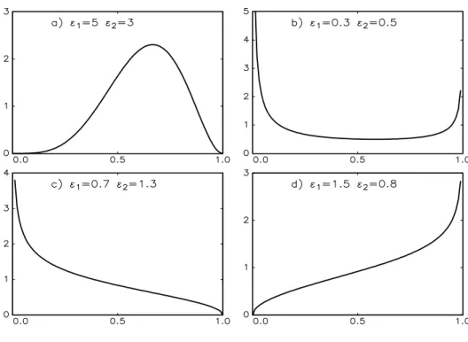
Figure 1: Beta distribution for various parameter combinations.

whereB(₁, ₂) = Γ(₁)Γ(₂)/Γ(₁+₂) is again the beta function, while the shape parameters are now given by

₁ =a₁/b and ₂ =a₂/b. (15) Figure 1 illustrates the flexibility in the shape of the beta distribution, with unimodal and bimodal cases similar to the symmetric case (11) in the top panel (a,b), but also including monotonically increasing or decreasing cases in situations where agents have a strong idiosyncratic signal in one direction, yet still exhibit a relatively pronounced herding tendency relative to the other state, i.e. a₁/b <1<

a₂/b or vice versa, as shown in the bottom panel (c,d).

In summary, the model provides quite a generic description of a stochastic ex- pectations formation process that contains only a few behavioral parametersa₁, a₂, and b, yet allows for a large degree of agent heterogeneity. Despite its parsimony, the model produces a wide range of qualitatively different statistical equilibria,

including endogenous cycles in expectations caused by herding or imitation, but also equilibria where the vast majority of agents ‘learns a correct state’ in spite of being surrounded by noise that is created through the social interaction with neighboring agents. The qualitative features of the process are also parsimoniously summarized by the ratios (12) or (15), putting us in a position to isolate behavioral aspects from the question whether it is feasible to identify the communication or network structure among agents from survey data.

In the next section we argue that an ‘omniscient modeler’, endowed with per- fect knowledge of the behavioral parameters and network structure among agents, would not be able to reliably recover this network structure based merely on the correlations in survey responses. Perhaps more troubling, if our knowledge is confined to the time evolution of survey responses, we will not even be able to reliably detect whether survey correlations originate from social interactions or model-consistent beliefs.

3 Random Benchmark and Simulation

We start with a thought experiment, putting ourselves in the position of an om- niscient modeler (OM) who chooses a particular behavioral setup and network structure for the model in Section 2. Utilizing the individual transition rates (1) and (2), the OM simulates and records the time evolution of beliefs for all N agents in the system. Afterwards, the OM presents us with data on the individual histories of agents’ beliefs (oroutput for short), from which we have to determine the network structure among agents based on correlations in the time evolution of their beliefs.

In actual data on survey expectations, with typically two to three hundred agents reporting monthly beliefs over roughly two hundred periods, we have no intrinsic knowledge of the network structure whatsoever. So to make life easier for us, the OM even informs us of the exact number D_i of neighbors for each agent i = 1, . . . , N. We then compute the D_i highest correlations for each agent from the output and report it back to the OM as our best guess of the network structure in the output. In return, the OM checks our guesses against the actual identity of neighbors and reveals the fraction of correctly identified neighbors to

us. The central question is: how many of the D_i neighbors do we expect to guess correctly by pure chance, i.e. irrespective of the correlation among responses?

This establishes a random benchmark against which we have to judge the success of correlation-based procedures.²

In order to explain the random benchmark, it is instructive to consider a simple urn model. Let us draw d (read: D_i) colored balls without replacement from an urn containing a total of N balls, m of which are white (read: the true neighbors of agent i). The probability of drawingk ≤m white balls in d draws from a total of N balls is given by the hypergeometric distribution

P(k) =

m k

N−m d−k

N d

, (16) where the notation on the right hand side refers to binomial coefficients. In other words, (16) characterizes the distribution of the number of white balls drawn from the urn in d extractions. The mean value of the hypergeometric distribution is

E[k] = dm

N , (17)

from which we can compute the random benchmark sinced=min our OM setup.³ The standard deviation of the hypergeometric distribution is

σ[k] = s

dm(N −m)(N −d)

(N −1)N² . (18)

To keep our simulations in line with available survey data (for instance from the ZEW for German ‘financial experts’, or from the FRB Philadelphia for US

‘professional forecasters’), we set the number of agents to N = 250; the available length of periods for individual agent IDs is on average between one and two hundred, while the number of questions per survey is typically between thirty and

2Instead of considering the time t correlation, we have conducted the subsequent analysis with various sums of leads and lags in the autocorrelations of responses, yet the results remain virtually unchanged.

3Notice that choosing a different number of extractions does not change any of the qualita- tive features in the following results, yet the approach immediately translates into quantitative prescriptions for measuring different benchmarks.

sixty. It will be a sobering experience to recall these figures when we present the simulation results.

3.1 Simulation setup

Regarding the network structure in our simulations, we consider three proto-typical setups: random graphs in the Erd¨os-Renyi tradition, scale-free networks in the Barabasi-Albert tradition, and regular lattice structures.⁴ To keep matters sim- ple, we set the number of neighbors equal to twenty in the lattice, and tune the parameters of the scale-free and random networks such that we obtain adjacency matrices with an average number of twenty neighbors as well.⁵ Given these num- bers and (17) and (18), it is straightforward to compute that the fraction of cor- rect answers we would expect purely by chance corresponds to E[k] = 1.6 with σ[k] = 1.16, or normalized with respect to the number of extractionsE[k]/d= 0.08 and σ[k]/d= 0.058.

In the subsequent figures, we use the mean plus one standard deviation, E[k] + σ[k] = 2.76, to illustrate the statistical significance of the OM experiment. We can compute the probability of such an event from the cumulative hypergeometric distribution: since the hypergeometric distribution is defined for positive integer values of k, we have to consider P(k ≤ 2) = 0.79 and P(k ≤ 3) = 0.94. Hence the range 0< E[k] +σ[k]<3 delivers a rather conservative confidence interval in accord with the usual econometric standards.

In line with (1), (2) and (13), the OM implements the transition probabilities φ_i for each agent i as

φ^(±)_i =ρ^(±)_i ∆t= [a_(1,2)+bD^(∓)_i ] ∆_t with ∆_t = 1/(a_max+bN), (19) where the notationD^(∓)_i refers to the number ofi-neighbors that are in the opposite state, and a_max = max{a1, a2}. The choice of ∆t ensures both that 0 < φ_i ≤ 1

4The review article by Newman (2003) provides the historical background and a comprehen- sive summary of the many mathematical details of these graphs.

5It turns out that changing the number of neighbors in the OM setup has virtually no influence on the subsequent results. We chose twenty neighbors because this figure does not appear to be entirely unrealistic. If anything, the communication with twenty neighbors already takes considerable time and effort in most professions.

and that all agents act on the same time scale.

The OM then confronts us with the output of the N time series of agents’

beliefs, from which we compute N(N −1)/2 correlation coefficients. For every i, the OM also informs us of the actual number D_i of neighbors, and in turn we extract the Di highest correlation coefficients from the output. Intuitively assuming that the highest correlation coefficients correspond to the neighbors of agent i, we construct the adjacency matrix of the agent network and report it to the OM who compares it with the actual adjacency matrix, and informs us of the fraction of correctly identified neighbors for eachi. To aggregate and visualize the results for each of the following three scenarios, we average the correctly identified percentages for each agent over the entire pool of agents.

The following scenarios basically consider in how far we can recover the correct network structure (i) depending on the length of agent histories and (ii) depending on the number of simultaneous survey answers per agent, i.e.the volume of survey coverage. The final scenario (iii) takes up a more fundamental issue and examines what happens when correlation clusters are caused by model-consistent beliefs in- stead of social interactions. Put differently, is a correlation-based approach capable of distinguishing between clusters that are caused by either behavioral extreme?

3.2 Scenario I: Single indicator histories

Suppose when agents answer questions regarding rather distant areas of expertise (e.g. international equity indices vs bonds vs GDP growth vs inflation etc.), they utilize different networks to form their expectations. So if we use histories for a single indicator in the OM experiment, what is the required number of observations per agent (or sample size for short) that is necessary to discriminate between some genuine network structure and random noise?

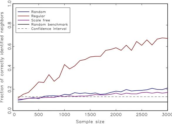
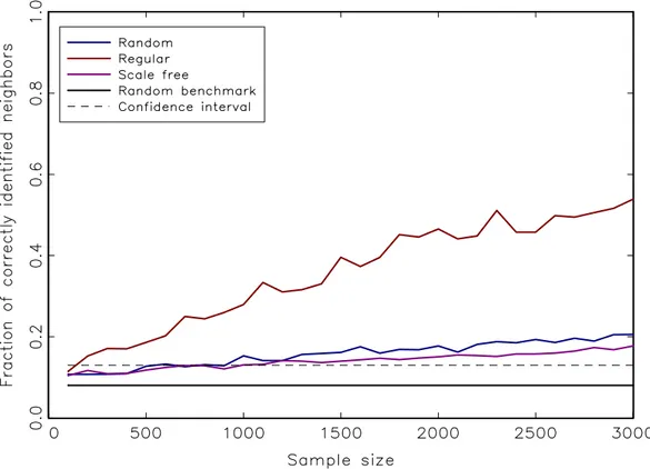
We consider both a bi- and a unimodal setup to control for behavioral biases, and display summary results under different network structures in Figures 2 and 3.

The figures illustrate that there is little difference between random and scale-free setups, while it is easier to identify neighbors when they are all arranged in a regular lattice. Regular networks, however, are the least suitable representation of observed social networks, which tend to interpolate between random and scale-free

Figure 2: Average fraction of correctly identified neighbors vs length of individual agents’ time series for a single question. We chose a bimodal simulation setup with parameters ε₁ =ε₂ =.5 and b = 1, i.e. a strong behavioral component relative to symmetric exogenous signals in either direction.

structures (see, e.g., Newman, 2003, and the references therein). This is also the reason why we focus our attention on random graphs in the coming scenarios.

As one would intuitively suspect, the identification of interaction effects is somewhat facilitated in the bimodal case, i.e.when herding or imitation dominate the expectations formation process. According to Figures 2 and 3, however, this aspect has merely second-order effects. Up to a sample size of around one thousand periods, we are not able to distinguish between noise and network effects if our knowledge is restricted to the time evolution of univariate histories. Hence this also implies that we do not have a sufficient number of empirical survey data at our disposal to reliably identify the social interaction component. Viewed from this perspective, any cluster we identify based on the cross-correlations of answers is

Figure 3: Average fraction of correctly identified neighbors vs length of individual agents’ time series for a single question. Here we chose a unimodal simulation setup with parameters ε₁ = ε₂ = 2 and b = 1, i.e. a relatively strong exogenous signal compared to the behavioral component.

essentially pure noise. If we consider the confidence interval in Figures 2 and 3, the first scenario suggests that it is entirely unrealistic to identify even a rudimentary communication structure unless we increase the frequency of survey responses by one order of magnitude, i.e.from monthly to roughly twice per week. In addition, if we are indeed facing irregular network structures, the length of single indicator histories that is necessary to correctly identify about half the neighbors turns out to be two orders of magnitude larger than empirical sample sizes.⁶

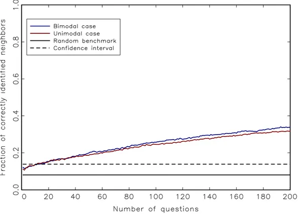
Figure 4: Increasing the number of questions and averaging over them improves the identification of interaction effects compared to the previous univariate sce- nario. The model parameterizations remain the same as before, and we utilize a random network whose structure remains fixed as well. The underlying univariate responses have a length of two hundred periods.

3.3 Scenario II: Multiple indicator histories

Can we improve the identification of communication structures if we make the strong assumption that behavioral parameters in the expectations formation pro- cess of agents do not change across multiple questions, and that their network structure remains unchanged as well? And how many questions would be nec- essary in that case? To tackle this issue, we keep the parameterizations of the previous scenario and simulate the expectations formation process on a random network, fixing the length of single question histories to two hundred while suc- cessively increasing the number of questions. Essentially, this means that the

6Simulation results upon request.

correlation coefficients are averaged both over agents and over questions. To op- erationalize this procedure, we fix the parameterization and underlying network structure of social interactions and run K independent simulations of the model for two hundred periods. For each single run of length two hundred, we perform the estimation procedure outlined in the previous scenario, and then average over the K questions.

The results both for uni- and bimodal setups, along with the random bench- mark, are displayed in Figure 4 and show that a multivariate correlation-based procedure performs better than in the previous univariate scenario. As expected, a bimodal environment with strong interactions again somewhat facilitates the identification of the network structure, but the more appealing feature of this sce- nario is that the rate at which we discover actual links is markedly higher than in the univariate case. On the downside, however, the overall accuracy of the correlation-based procedure remains low. Keeping in mind that the empirical vol- ume of survey coverage includes roughly thirty to sixty questions, correlation-based estimates of the interaction structure are almost not significantly different from pure noise, and certainly very low to begin with: we recover merely twenty percent of the actual network structure, and the fraction of correctly identified neighbors increases very slowly with the number of questions.

3.4 Scenario III: Exogenously switching signal

In both of the preceding scenarios we have assumed that all agents have a strictly positive interaction parameter, which we conveniently set to b = 1. But what happens if some agents are not socially interacting at all (b = 0) and instead form model-consistent beliefs from exogenous signals a₁, a₂ that we can think of as transmitting the correct state of the world? In principle, these ‘rational’ agents should exhibit highly correlated responses over time if the exogenous signal is sufficiently strong relative to the interaction parameter. If the state of the world does not change over time, the rational agents will all converge to the correct state, making it almost trivial to identify them from correlation-based procedures. In order to maintain an empirically more relevant scenario, we thus assume that the correct state of the world changes every now and then, i.e. the parameters a₁, a₂

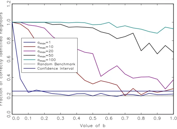
Figure 5: Fraction of correctly identified rational agents who follow a time-varying exogenous signal that is increasingly biased in either direction (denoted by an increasing value of a_max) vs their interaction strength b. At low values of b, the identification generally performs very well, while higher values ofb might prevent a reliable detection, depending on the relative value of a_max.

are no longer constant but change over time.⁷

In this scenario, we keep the total number of agents at N = 250 in our sim- ulations, and the underlying network remains a random graph with an average degree of twenty neighbors. The values of ˜a₁ = ˜a₂ = ˜b = 1 are constant over time for the majority ˜N = 200 of agents, while a smaller group of fifty ‘rational’

agents exhibits time-varying idiosyncratic coefficients, say a₁(t) and a₂(t), which essentially measure the speed at which rational agents learn the true state of the world. The time-varying coefficients take on values in the set {1, a_max}, where a_max = max{a₁(t), a₂(t)}. Suppose for instance that a_max = 10 and that the

7From a mathematical point of view, this would correspond to a so-calledswitching diffusion process.

currently ‘true’ state is such that a₁(0) = 1 and a₂(0) = 10, i.e. we are in an optimistic regime today. When the true state changes to pessimism, say in period τ, the parameters change to a₁(τ) = 10 and a₂(τ) = 1. As far as the switch- ing probability in our simulations is concerned, we assume that the probability to switch is five percent, drawn randomly from a uniform distribution. In other words, an exogenous switch in the signal occurs on average every twenty months in our simulations.

The matter in question now concerns the fraction of rational agents that we can correctly identify if the true state of the world changes over time, as it certainly does in reality. (Notice that we have to adapt the error band since now d =m= 50.) None the less, we would expect the value of b to also have an influence on our ability to identify the rational agents: when b increases, the noise generated through the social interactions with the other agents should make it more difficult to identify rational agents correctly. On the other hand, when rational agents are not part of the social network (b = 0), and thus do not take possibly non- rational opinons into account, it should become easier to correctly identify them with correlation-based procedures.

Figure 5 plots the fraction of correctly identified rational agents for a given a_max when the interaction parameterb takes on values in [0,1]. The different plots in Figure 5 refer to increasing values of a_max in the simulations. As expected, our ability to correctly identify the group of rational agents depends inversely on their interaction parameterb, possibly approaching the noise level as bapproaches the value common to the other ˜N agents. On the other hand, whenb approaches zero, we are in an increasingly comfortable position regarding the identification of rational agents. Finally, the faster the signal processing ability a_max, the easier it becomes to correctly identify the group of rational agents, asymptotically reaching the value of one hundred percent independently of b.

4 Discussion and Conclusions

All computations in the preceding scenarios have been performed under the as- sumption that the OM informs us of the actual number Di of neighbors for each agent. Clearly, this is a most unrealistic assumption in the context of empirical

applications to survey data, where we simply have no way of knowing whether agents interact socially in the first place, much less to whom they are linked to in case they do. Viewed from this perspective, our results are if anything overly optimistic to begin with.

Yet the third scenario delivers maybe the most fatal blow to any hopes that survey data could settle the question whether interaction effects are present in the expectations formation process of respondents or not. Our preferred way to read Figure 5 is that we can achieve any desired accuracy in the identification of network structure through an appropriate combination of b and a time-varying exogenous signal a_max. The other side of that coin is that we have no way of distinguishing between interaction effects and model-consistent beliefs, even if we identify relatively strong patterns in the correlations of a subset of agents.

Ultimately, these results suggest that existing survey data cannot facilitate our understanding of the process of expectations formation, which is particularly troubling in light of its central importance for modern macroeconomic theory. To end on a more constructive note, we would like to point out once more that our thought experiment presumed that we merely have data on the time evolution of agents’ beliefs. In order to investigate whether interaction effects are indeed present in the data, it would be enormously helpful if surveys contained questions that refer directly to the presence of interaction effects.

References

S. Alfarano and M. Milakovi´c. Network structure and N-dependence in agent- based herding models. Journal of Economic Dynamics and Control, 33:78–92, 2009.

S. Alfarano, T. Lux, and F. Wagner. Estimation of agent-based models: The case of an asymmetric herding model. Computational Economics, 26:19–49, 2005.

S. Alfarano, T. Lux, and F. Wagner. Time-variation of higher moments in a financial market with heterogeneous agents: An analytical approach. Journal of Economic Dynamics and Control, 32:101–136, 2008.

M. Aoki. New Approaches to Macroeconomic Modeling. Cambridge University Press, Cambridge, UK, 1998.

M. Bowden and S. McDonald. The impact of interaction and social learning on aggregate expectations. Computational Economics, 31(3):289–306, 2008.

W. A. Brock and S. N. Durlauf. Discrete choice with social interactions. Review of Economic Studies, 68(2):235–60, 2001.

C. D. Carroll. Macroeconomic expectations of households and professional fore- casters. Quarterly Journal of Economics, 118(1):269–298, 2003.

M. P. Clements. Explanations of the inconsistencies in survey respondents’ fore- casts. European Economic Review, 54(4):536–549, 2010.

O. Coibion and Y. Gorodnichenko. What can survey forecasts tell us about infor- mational rigidities? NBER Working Paper 14586, National Bureau of Economic Research, December 2008.

M. Del Negro and S. Eusepi. Modeling observed inflation expectations. mimeo, Federal Reserve Bank of New York, 2009.

G. Evans and S. Honkapohja. Learning and Expectations in Macroeconomics.

Princeton University Press, Princeton, 2001.

B. Flieth and J. Foster. Interactive expectations. Journal of Evolutionary Eco- nomics, 12(4):375–395, 2002.

C. H. Hommes. The heterogeneous expectations hypothesis: Some evidence from the lab. mimeo, University of Amsterdam, Netherlands, 2010.

A. Kirman. Epidemics of opinion and speculative bubbles in financial markets. In M. P. Taylor, editor, Money and Financial Markets, pages 354–368. Blackwell, Cambridge, 1991.

A. Kirman. Ants, rationality, and recruitment. Quarterly Journal of Economics, 108:137–156, 1993.

M. Lines and F. Westerhoff. Inflation expectations and macroeconomic dynamics:

The case of rational versus extrapolative expectations. Journal of Economic Dynamics and Control, 34:246–257, 2010.

T. Lux. Rational forecasts or social opinion dynamics? Identification of inter- action effects in a business climate survey. Journal of Economic Behavior and Organization, 72(2):638–655, 2009.

N. G. Mankiw and R. Reis. Sticky information versus sticky prices: A proposal to replace the New Keynesian Phillips curve. Quarterly Journal of Economics, 117(4):1295–1328, 2002.

N. G. Mankiw, R. Reis, and J. Wolfers. Disagreement about inflation expectations.

In NBER Macroeconomics Annual 2003, volume 18, pages 209–270, Cambridge, July 2004. MIT Press.

F. Milani. Expectation shocks and learning as drivers of the business cycle. CEPR Discussion Paper 7743, Centre for Economic Policy Research, March 2010.

M. Newman. The structure and function of complex networks. SIAM Review, 45:

167–256, 2003.

M. H. Pesaran and M. Weale. Survey expectations. In G. Elliott, C. Granger, and A. Timmermann, editors, Handbook of Economic Forecasting, volume 1, chapter 14, pages 715–776. Elsevier, 2006.

C. A. Sims. Implications of rational inattention. Journal of Monetary Economics, 50(3):665–690, 2003.

W. Weidlich. Sociodynamics: A Systemic Approach to Mathematical Modelling in the Social Sciences. Dover, New York, 2006.

W. Weidlich and G. Haag. Concepts and Methods of a Quantitative Sociology.

Springer, Berlin, 1983.

M. Woodford. Imperfect common knowledge and the effects of monetary policy.

In Knowledge, Information, and Expectations in Modern Macroeconomics: In

Honor of Edmund S. Phelps, chapter 1, pages 25–58. Princeton University Press, Princeton, 2001.

BERG Working Paper Series on Government and Growth

1 Mikko Puhakka and Jennifer P. Wissink, Multiple Equilibria and Coordination Failure in Cournot Competition, December 1993

2 Matthias Wrede, Steuerhinterziehung und endogenes Wachstum, December 1993 3 Mikko Puhakka, Borrowing Constraints and the Limits of Fiscal Policies, May 1994 4 Gerhard Illing, Indexierung der Staatsschuld und die Glaubwürdigkeit der Zentralbank in

einer Währungsunion, June 1994

5 Bernd Hayo, Testing Wagner`s Law for Germany from 1960 to 1993, July 1994

6 Peter Meister andHeinz-Dieter Wenzel, Budgetfinanzierung in einem föderalen System, October 1994

7 Bernd Hayo and Matthias Wrede, Fiscal Policy in a Keynesian Model of a Closed Monetary Union, October 1994

8 Michael Betten, Heinz-Dieter Wenzel, and Matthias Wrede, Why Income Taxation Need Not Harm Growth, October 1994

9 Heinz-Dieter Wenzel (Editor), Problems and Perspectives of the Transformation Process in Eastern Europe, August 1995

10 Gerhard Illing, Arbeitslosigkeit aus Sicht der neuen Keynesianischen Makroökonom ie, September 1995

11 Matthias Wrede, Vertical and horizontal tax competition: Will uncoordinated Leviathans end up on the wrong side of the Laffer curve? December 1995

12 Heinz-Dieter Wenzel and Bernd Hayo, Are the fiscal Flows of the European Union Budget explainable by Distributional Criteria? June 1996

13 Natascha Kuhn, Finanzausgleich in Estland: Anal yse der bestehenden Struktur und Ü- berlegungen für eine Reform, June 1996

14 Heinz-Dieter Wenzel, Wirtschaftliche Entwicklungsperspektiven Turkm enistans, July 1996

15 Matthias Wrede, Öffentliche Verschuldung in einem föderalen Staat; Stabilität, vertikale Zuweisungen und Verschuldungsgrenzen, August 1996

17 Heinz-Dieter Wenzel and Bernd Hayo, Budget and Financial Planning in Germany, Feb- ruary 1997

18 Heinz-Dieter Wenzel, Turkmenistan: Die ökonomische Situation und Perspektiven wirt- schaftlicher Entwicklung, February 1997

19 Michael Nusser, Lohnstückkosten und internationale W ettbewerbsfähigkeit: Eine kriti- sche Würdigung, April 1997

20 Matthias Wrede, The Competition and Federalism - The Underprovision of Local Public Goods, September 1997

21 Matthias Wrede, Spillovers, Tax Competition, and Tax Earmarking, September 1997 22 Manfred Dauses, Arsène Verny, Jiri Zemánek, Allgemeine Methodik der Rechtsanglei-

chung an das EU-Recht am Beispiel der Tschechischen Republik, September 1997 23 Niklas Oldiges, Lohnt sich der Blick über den Atlan tik? Neue Perspektiven für die aktu-

elle Reformdiskussion an deutschen Hochschulen, February 1998

24 Matthias Wrede, Global Environmental Problems and Actions Taken by Coalitions, May 1998

25 Alfred Maußner, Außengeld in berechenbaren Konjunkturm odellen – Modellstrukturen und numerische Eigenschaften, June 1998

26 Michael Nusser, The Implications of Innovations and W age Structure Rigidity on Eco- nomic Growth and Unem ployment: A Schumpetrian Approach to Endogenous Growth Theory, October 1998

27 Matthias Wrede, Pareto Efficiency of the Pay-as-you-go Pension System in a Three- Period-OLG Modell, December 1998

28 Michael Nusser, The Implications of Wage Structure Rigidity on Hum an Capital Accu- mulation, Economic Growth and Unem ployment: A Schum peterian Approach to En- dogenous Growth Theory, March 1999

29 Volker Treier, Unemployment in Reforming Countries: Causes, Fiscal Im pacts and the Success of Transformation, July 1999

30 Matthias Wrede, A Note on Reliefs for Traveling Expenses to Work, July 1999

31 Andreas Billmeier, The Early Years of Inflation Targeting – Review and Outlook –, Au- gust 1999

33 Matthias Wrede, Mobility and Reliefs for Traveling Expenses to Work, September 1999 34 Heinz-Dieter Wenzel (Herausgeber), Aktuelle Fragen der Finanzwissenschaft, February

2000

35 Michael Betten, Household Size and Household Utility in Intertemporal Choice, April 2000

36 Volker Treier, Steuerwettbewerb in Mittel- und Os teuropa: Eine Einschätzung anhand der Messung effektiver Grenzsteuersätze, April 2001

37 Jörg Lackenbauer und Heinz-Dieter Wenzel, Zum Stand von Transformations- und EU- Beitrittsprozess in Mittel- und Osteuropa – eine komparative Analyse, May 2001

38 Bernd Hayo und Matthias Wrede, Fiscal Equalisation: Principles and an Application to the European Union, December 2001

39 Irena Dh. Bogdani, Public Expenditure Planning in Albania, August 2002

40 Tineke Haensgen, Das Kyoto Protokoll: Eine ökonom ische Analyse unter besonderer Berücksichtigung der flexiblen Mechanismen, August 2002

41 Arben Malaj and Fatmir Mema, Strategic Privatisation, its Achievem ents and Chal- lenges, Januar 2003

42 Borbála Szüle 2003, Inside financial conglom erates, Effects in the Hungarian pension fund market, January 2003

43 Heinz-Dieter Wenzel und Stefan Hopp (Herausgeber), Seminar Volume of the Second European Doctoral Seminar (EDS), February 2003

44 Nicolas Henrik Schwarze, Ein Modell für Finanzkrisen bei Moral Hazard und Überin- vestition, April 2003

45 Holger Kächelein, Fiscal Competition on the Local Level – May commuting be a source of fiscal crises?, April 2003

46 Sibylle Wagener, Fiskalischer Föderalismus – Theoretische Grundlagen und Studie Un- garns, August 2003

47 Stefan Hopp, J.-B. Say’s 1803 Treatise and the Coordination of Economic Activity, July 2004

48 Julia Bersch, AK-Modell mit Staatsverschuldung und fixer Defizitquote, July 2004

50 Heinz-Dieter Wenzel, Jörg Lackenbauer,and Klaus J. Brösamle, Public Debt and the Future of the EU's Stability and Growth Pact, December 2004

51 Holger Kächelein, Capital Tax Competition and Partial Cooperation: Welfare Enhancing or not? December 2004

52 Kurt A. Hafner, Agglomeration, Migration and Tax Competition, January 2005

53 Felix Stübben, Jörg Lackenbauer und Heinz-Dieter Wenzel,Eine Dekade wirtschaftli- cher Transformation in den Westbalkanstaaten: Ein Überblick, November 2005

54 Arben Malaj, Fatmir Mema andSybi Hida, Albania, Financial Management in the Edu- cation System: Higher Education, December 2005

55 Osmat Azzam, Sotiraq Dhamo and Tonin Kola, Introducing National Health Accounts in Albania, December 2005

56 Michael Teig, Fiskalische Transparenz und ökonom ische Entwicklung: Der Fall Bos- nien-Hercegovina, März 2006

57 Heinz-Dieter Wenzel (Herausgeber), Der Kaspische Raum : Ausgewählte Them en zu Politik und Wirtschaft, Juli 2007

58 Tonin Kola and Elida Liko, An Em pirical Assessment of Alternative Exchange Rate Regimes in Medium Term in Albania, Januar 2008

59 Felix Stübben, Europäische Energieversorgung: Status quo und Perspektiven, Juni 2008 60 Holger Kächelein, Drini Imami and Endrit Lami, A new view into Political Business

Cycles: Household Expenditures in Albania, July 2008

61 Frank Westerhoff, A simple agent-based financial market model: direct interactions and comparisons of trading profits, January 2009

62 Roberto Dieci and Frank Westerhoff, A simple model of a speculative housing m arket, February 2009

63 Carsten Eckel,International Trade and Retailing, April 2009

64 Björn-Christopher Witte, Temporal information gaps and market efficiency: a dynam ic behavioral analysis, April 2009

65 Patrícia Miklós-Somogyi and László Balogh, The relationship between public balance

66 H.-Dieter Wenzel und Jürgen Jilke, Der Europäische Gerichtshof EuGH als Brem sklotz einer effizienten und koordinierten Unternehm ensbesteuerung in Europa? , November 2009

67 György Jenei, A Post-accession Crisis? Political Developm ents and Public Sector Mod- ernization in Hungary, December 2009

68 Marji Lines and Frank Westerhoff, Effects of inflation exp ectations on macroeconomic dynamics: extrapolative versus regressive expectations, December 2009

69 Stevan Gaber, Economic Implications from Deficit Finance, January 2010

70 Abdulmenaf Bexheti, Anti-Crisis Measures in the Republic of Macedonia and their Ef- fects – Are they Sufficient?, March 2010

71 Holger Kächelein, Endrit Lami and Drini Imami, Elections Related Cycles in Publicly Supplied Goods in Albania, April 2010

72 Annamaria Pfeffer, Staatliche Zinssubvention und Au slandsverschuldung: Eine Mittel- wert-Varianz-Analyse am Beispiel Ungarn, April 2010

73 Arjan Tushaj, Market concentration in the banking sector: Evidence from Albania, April 2010

74 Pál Gervai, László Trautmann and Attila Wieszt, The mission and culture of the corpo- ration, October 2010

75 Simone Alfarano and Mishael Milaković, Identification of Interaction Effects in Survey Expectations: A Cautionary Note, October 2010