Heterogeneous Expectations and Complex Economic Dynamics

Heterogeneous Expectations and Complex Economic Dynamics

Dissertation

noemi schmitt

Submitted to the University of Bamberg

Diese Arbeit hat der Fakult¨ at Sozial- und Wirtschaftswissenschaften der Otto- Friedrich-Universit¨ at Bamberg als kumulative Dissertation vorgelegen.

1. Gutachter: Prof. Dr. Frank Westerhoff 2. Gutachter: Prof. Dr. Christian Proa˜ no 3. Gutachter: Prof. Dr. Guido Heineck Tag der m¨ undlichen Pr¨ ufung: 20.04.2018

URN: urn:nbn:de:bvb:473-opus4-518076

DOI: https://doi.org/10.20378/irbo-51807

SYNOPSIS

The expectation formation behavior of heterogeneous and boundedly rational agents may create complex economic dynamics. This doctoral thesis seeks to explain how such dynamics may arise and how they may be regulated.

The first part of the thesis consists of two papers in which we analyze whether policy-makers can stabilize markets by imposing profit taxes. For this purpose, the seminal cobweb model by Brock and Hommes is considered. Within their model, firms adapt their price expectations by a profit-based switching behavior between free naive expectations and costly rational expectations. They demonstrate that fixed-point dynamics may turn into increasingly complex dynamics as the firms’

intensity of choice increases. In Paper 1 it is shown that policy-makers may be able to manage such rational routes to randomness by imposing a proportional tax on positive profits. The basic idea is that an increase in the tax rate reduces profit differentials between the two expectation rules. As a result, more firms rely on rational expectations which brings stability to the market. Unfortunately, the stability-ensuring profit tax rate increases with the firms’ intensity of choice, and may become quite high. Since a high tax burden may be harmful for firms, an alternative tax function is considered in Paper 2. Here it is shown that a rather small profit-dependent lump-sum tax may even be sufficient to take away the competitive edge of cheap destabilizing expectation rules, thereby contributing to market stability.

The second part, comprising five papers, seeks to improve our understanding

of how financial markets function. The goal of each of these papers is to develop a

simple agent-based financial market model that is able to explain the stylized facts

of stock markets. Although all of them are related, each has its own focus. In Paper

3, speculators rely on technical and fundamental analysis to determine their orders

and have the opportunity to trade on two different stock markets. Their choices are

repeated in each time step and depend on predisposition effects, herding behavior

and market circumstances. Simulations reveal that this setup is able to explain

a number of nontrivial statistical properties of and between international stock

markets. Paper 4 considers a single stock market which investors can enter. It is assumed that stock market participation depends on current market movements and on the fundamental state of the market, i.e. investors tend to enter (exit) the market in periods of increasing (decreasing) stock prices and exit (enter) the market in periods of overvaluation (undervaluation). We demonstrate that changes in stock market participation may lead to endogenous boom-bust dynamics. Paper 5 shows that volatility clustering may arise due to speculators’ herding behavior.

To be more precise, speculators observe other speculators’ actions more closely in periods of heightened uncertainty. Since speculators’ trading behavior then becomes less heterogeneous, the market maker faces a less balanced excess demand and consequently adjusts prices more strongly. Estimating this model reveals that it explains the dynamics of financial markets quite well. The model developed in Paper 6 is a very simple large-scale model in which speculators usually follow their own individual technical and fundamental trading rules. However, there are also sunspot-initiated periods in which their trading behavior is correlated. Under a few assumptions, this framework can be converted into a small-scale model which makes it possible to bring the framework to the data. As it turns out, the small-scale model has a remarkable ability to match the stylized facts of financial markets. Paper 7 provides an agent-based micro-foundation of the seminal asset pricing model by Brock and Hommes. Within their elementary setup, agents choose between a representative technical and a representative fundamental expectation rule. Since agents’ expectations differ in reality, their framework is generalized by considering that all agents follow their own time-varying technical and fundamental expectation rules. The analysis reveals that heterogeneity is not only a realistic model property but clearly helps to explain the intricate dynamics of financial markets.

Each of these seven papers is independent from each other and can be read with-

out any prior knowledge of the others. The first six papers were jointly written with

my Ph.D. supervisor Frank Westerhoff and were published in the Journal of Eco-

nomic Behavior & Organization, Macroeconomic Dynamics, Journal of Economic

Dynamics & Control, Economics Letters, Quantitative Finance and the Journal of

Evolutionary Economics. The last paper has not been published yet.

CONTENTS

Part I. Cobweb models

Paper 1. Managing rational routes to randomness, with Frank Westerhoff, Journal of Economic Behavior & Organization (2015), 116, 157-173.

Paper 2. Evolutionary competition and profit taxes: market sta- bility versus tax burden, with Frank Westerhoff, Macroeconomic Dynamics (2016), in press.

Part II. Financial market models

Paper 3. Speculative behavior and the dynamics of interacting stock markets, with Frank Westerhoff, Journal of Economic Dy- namics & Control (2014), 45, 262-288.

Paper 4. Stock market participation and endogenous boom-bust dynamics, with Frank Westerhoff, Economics Letters (2016), 148, 72-75.

Paper 5. Herding behaviour and volatility clustering in financial markets, with Frank Westerhoff, Quantitative Finance (2017), 17, 1187-1203.

Paper 6. Heterogeneity, spontaneous coordination and extreme events within large-scale and small-scale agent-based financial mar- ket models, with Frank Westerhoff, Journal of Evolutionary Eco- nomics (2017), 27, 1041-1070.

Paper 7. Heterogeneous expectations and asset price dynamics,

Working Paper (2017), University of Bamberg.

PART I

Managing rational routes to randomness

Paper 1

This article has already been published in the Journal of Economic Behavior & Organization 116 (2015), 157–173:

http://dx.doi.org/10.1016/j.jebo.2015.04.018

Evolutionary competition and profit taxes: market stability

versus tax burden

Paper 2

This article has already been published in Macroeconomic Dynamics (2016), in press:

https://doi.org/10.1017/S1365100516000985

PART II

Speculative behavior and the dynamics of interacting stock

markets

Paper 3

This article has already been published in the Journal of Economic Dynamics & Control 45 (2014), 262–288:

http://dx.doi.org/10.1016/j.jedc.2014.05.009

Stock market participation and endogenous boom-bust dynamics

Paper 4

This article has already been published in Economics Letters 148 (2016), 72–75:

http://dx.doi.org/10.1016/j.econlet.2016.09.016

Herding behaviour and volatility clustering in financial markets

Paper 5

This article has already been published in Quantitative Finance 17 (2017), 1187–1203:

https://doi.org/10.1080/14697688.2016.1267391

Heterogeneity, spontaneous coordination and extreme events within large-scale and small-scale

agent-based financial market models

Paper 6

This article has already been published in the Journal of Evolutionary Economics 27 (2017), 1041–1070:

https://doi.org/10.1007/s00191-017-0504-x

Heterogeneous expectations and asset price dynamics

Paper 7

Heterogeneous expectations and asset price dynamics

Noemi Schmitt*

University of Bamberg, Department of Economics, Feldkirchenstrasse 21, 96045 Bamberg, Germany

Abstract

Within the seminal asset-pricing model by Brock and Hommes (1998), heterogeneous boundedly rational agents choose between a fixed number of expectation rules to forecast asset prices. However, agents’ heterogeneity is limited in the sense that they typically switch between a representative technical and a representative fundamental expectation rule. Here we generalize their framework by considering that all agents follow their own time-varying technical and fundamental expectation rules. Estimating our model using the method of simulated moments reveals that it is able to explain the statistical prop- erties of the daily behavior of the S&P500 quite well. Moreover, our analysis reveals that heterogeneity is not only a realistic model property but clearly helps to explain the intricate dynamics of financial markets.

Keywords: Financial markets, stylized facts, agent-based models, technical and fundamental analysis, heterogeneity and coordination

JEL classification: C63, D84, G15

1. Introduction

One of the most influential asset-pricing models with heterogeneous beliefs is the one by Brock and Hommes (1998). In their setup, agents choose from a finite set of different expectation rules to forecast prices and update their choices according to past realized profits. Moreover, agents are boundedly rational in the sense that they tend to switch toward forecasting strategies that have performed better in the past. A main result

∗

noemi.schmitt@uni-bamberg.de

offered by their model is that complicated asset price dynamics may arise when the intensity of choice to switch predictors is high. The evolutionary predictor selection approach has also been used by Brock and Hommes (1997), who call the bifurcation route to increasingly complex dynamics as the intensity of choice to switch forecasting strategies increases a rational route to randomness.

Due to their power and great economic appeal, the models by Brock and Hommes (1997, 1998) have been extended in various interesting directions. For instance, Brock et al. (2009) introduce Arrow securities and demonstrate that adding more hedging instruments may destabilize market dynamics. Similarly, Anufriev and Tuinstra (2013) introduce short-selling constraints to analyze whether such a policy measure can stabilize financial markets. In de Grauwe and Grimaldi (2006), the switching mechanism is implemented in a non-linear exchange rate model and it is shown that important features of exchange rates can be reproduced. Of course, many more extensions exist in the literature. See Hommes (2013) for an excellent review. Note also that Boswijk et al.

(2003), using yearly S&P500 data, and Hommes and in’t Veld (2017), using quarterly S&P500 data, provide strong empirical support for the approach by Brock and Hommes (1998).

In the most elementary version of their model, all agents switch between a represen- tative technical and a representative fundamental expectation rule. In reality, however, agents’ expectations differ. Empirical studies, such as the ones by Ito (1990), MacDon- ald and Marsh (1996), Menkhoff et al. (2009) or Jongen et al. (2012), explicitly stress that expectations of professional forecasters are heterogeneous. Anufriev and Hommes (2012), reinvestigating the laboratory experiments of Hommes et al. (2005, 2008), also find that heterogeneous expectations are crucial to describe the boom-and-bust dynam- ics of financial markets. However, forecasters’ behavior is not independent. A striking and robust finding of the learning to forecast experiment by Hommes et al. (2005) is that individuals tend to coordinate on using the same type of simple prediction strategies.

Furthermore, speculators are subject to herding behavior, which has already been docu- mented in several empirical studies. Trueman (1994), for instance, analyzes forecasts by financial analysts and reports that they tend to release forecasts similar to those released by others. Welch (2000) also detects a positive influence of security analysts’ buy or sell

2

recommendations on those of others. Note that a number of agent-based financial mar- ket address speculators’ herding behavior, see, for instance, Kirman (1993), Lux (1995) or Cont and Bouchaud (2000).

Against this background, we want to generalize the framework by Brock and Hommes (1998) by considering that all agents follow their own time-varying technical and fun- damental expectation rules, i.e. we assume that all agents have different expectations.

Since speculators do not trade independently from each other, we also assume that our agents’ forecasts are correlated. Thus, the first goal of this contribution is to provide an agent-based microfoundation of the model by Brock and Hommes (1998). Moreover, we want to explore the extent to which the generalized model can explain the stylized facts of financial markets. For this purpose, we estimate our model using the method of simulated moments and find that our approach matches the daily behavior of the S&P500 quite well. In this sense, our paper complements the studies by Boswijk et al.

(2003) and Hommes and in’t Veld (2017), who rely on yearly and quarterly S&P500 data, respectively. Finally, our analysis also reveals a novel explanation for the intricate behavior of financial markets. As we will see, the simplicity of our approach allows analytical insights that prove to be helpful in understanding how the model functions.

Related to our approach is the work by Brock et al. (2005) in which the model by Brock and Hommes (1998) is generalized to an evolutionary system with many different trader types. It is shown that the evolutionary dynamics can be approximated by the notion of a large type limit (LTL) in the sense that all generic and persistent features of an evolutionary system with many trader types, such as steady state, local bifurcations or (quasi-)periodic dynamics, also occur in the LTL system. LeBaron et al. (1999) develop an artificial stock market model in which a large number of interacting agents can choose from many different forecasting rules. As it turns out, their model is able to replicate certain stylized facts of stock markets. However, analytical tractability is impossible in such a framework. Of course, many other agent-based financial market models aim to explain the stylized facts of financial markets. For general surveys, see, for example, LeBaron (2006), Chiarella et al. (2009) or Lux (2009).

The remainder of this paper is organized as follows. In Section 2, we extend the seminal model by Brock and Hommes (1998) by assuming that all agents have heteroge-

3

neous expectations. After presenting the setup of our model, we analyze its deterministic skeleton in Section 3. In particular, we derive the dynamical system of our deterministic model and analyze its steady states and their local asymptotic stability. In Section 4, we estimate our model and demonstrate that the stochastic version of our model replicates a number of important stylized facts of financial markets. Section 5 concludes our paper and highlights a few avenues for future research.

2. Model setup

In this section, we consider the asset pricing model with heterogeneous boundedly ratio- nal agents by Brock and Hommes (1998) and provide an agent-based micro-foundation of their setup. They assume that agents know the risky asset’s fundamental value but choose from a finite set of different beliefs to forecast its price. In their elementary setup, these rules comprise a single fundamental and a single technical prediction rule.

Agents’ choices are updated in each period and depend on the past performance of the forecasting rules. In contrast to Brock and Hommes (1998), we assume that each agent follows his own fundamental and technical prediction rule, i.e. all agents have different expectations. However, agents’ forecasts are correlated to some extent.

Let us turn to the details of the model. Agents can invest in a risk-free asset or in a risky asset. The risk-free asset is in perfectly elastic supply and pays a fixed rate of return r, while the risky asset is in zero net supply and pays an uncertain dividend y

. By defining p

as the price per share (ex-dividend) of the risky asset at time t, the wealth of agent i in period t + 1 can be expressed as

W

= (1 + r)W

+ (p

+ y

− (1 + r)p

)z

, (1) where z

represents the demand of agent i for the risky asset at time t. Since agents are assumed to behave as myopic mean-variance maximizers, their demand for the risky asset follows from

max

z_tⁱ

{E

[W

] − a

2 V

[W

]}, (2)

where E

[W

] and V

[W

] denote agent i’s beliefs about the conditional expectation and conditional variance of his wealth in period t + 1 and parameter a represents a

4

uniform risk aversion coefficient. Moreover, it is assumed that beliefs about conditional variance are constant and uniform across all agents, i.e. V

[p

+ y

− (1 + r)p

] = σ

for all t and agents i.

Solving (2) for z

then yields

z

= E

[p

+ y

− (1 + r)p

]

aV

[p

+ y

− (1 + r)p

] = E

[p

+ y

− (1 + r)p

]

aσ

. (3)

As in Brock and Hommes (1998), the supply of shares per agent is denoted by z

and is assumed to be fixed. Equilibrium of demand and supply can therefore be formalized as

N

X

i=1

E

[p

+ y

− (1 + r)p

]

aσ

= N z

, (4)

where N denotes the total number of agents. By assuming a zero supply of outside shares, i.e. z

= 0,

the market equilibrium equation becomes

(1 + r)p

= P

i=1

E

[p

+ y

]

N . (5)

Before agents’ expectations about future prices and dividends are specified, let us recall how the fundamental price is derived. When all agents have homogeneous expec- tations, equation (5) simplifies to

(1 + r)p

= E

[p

+ y

], (6) which can be used repeatedly. If a perfectly rational world is then assumed and the transversality condition

t→∞

lim

E

[p

]

(1 + r)

= 0 (7)

holds, the fundamental price can be determined by the discounted sum of expected

1

Gaunersdorfer (2000) studies the case in which agents’ beliefs about conditional variances are time- varying and observes, at least in the case of an IID dividend process, similar dynamics as in the original model by Brock and Hommes (1998).

2

Brock (1997) gives a justification for the simplifying case

= 0 by introducing risk-adjusted dividends.

5

future dividends, i.e.

p

=

∞

X

k=1

E

[y

]

(1 + r)

. (8)

Since Brock and Hommes (1998) consider an IID dividend process y

with mean E[y

] =

¯

y, the fundamental price is constant and given by

p

=

∞

X

k=1

¯ y

(1 + r)

= y ¯

r . (9)

Expectations about future dividends are assumed to be identical across all agents and correspond to the conditional expectation, i.e.

E

[y

] = E

[y

] = ¯ y, (10) which also implies that all agents know the fundamental value p

that would prevail in a perfectly rational world. However, the equilibrium price can then be expressed as

p

= 1 1 + r (¯ y +

P

i=1

E

[p

]

N ). (11)

Brock and Hommes (1998) assume that expectations about future prices are hetero- geneous and consider various types of belief. In this paper, we assume that agents choose among two general types of forecasting rules, i.e. agents can either rely on technical or on fundamental analysis to predict prices.

This can be formalized by

E

[p

] =



 

 

E

[p

] if I

= 1 E

[p

] if I

= 0

, (12)

where E

[p

] and E

[p

] represent agent i’s price forecasts by using technical and fundamental analysis, respectively. Accordingly, agent i chooses the technical (funda- mental) prediction rule when the indicator function I

takes the value 1 (0).

Technical analysis seeks to extrapolate past price trends into the future (Murphy

3

Questionnaire studies by Menkhoff and Taylor (2007) and laboratory experiments by Hommes (2011) strongly support this assumption.

6

1999), while fundamentalists believe that asset prices revert towards their fundamental value (Graham and Dodd 1951). Since there is a wide variety of technical and funda- mental forecasting rules, we follow Westerhoff and Dieci (2006) and Franke (2010) and capture at least part of the rules’ heterogeneity by adding noise components to the basic principles. In contrast to their model setups, however, the noise affects agents on an individual level, which implies that all agents have different expectations. Accordingly, agent i’s technical and fundamental price forecasts consist of two components and are specified by

E

[p

] = p

+ (1 − g)(p

− p

) + p

σ

(13) and

E

[p

] = p

+ (1 − v)(p

− p

) + p

σ

, (14) respectively. The first parts of (13) and (14) represent the core principles of the forecast- ing rules, where g and v denote the coefficients of the two types of belief. As can be seen, both forecasting rules predict the next period’s price by extrapolating past deviations from the fundamental value. If agents follow the technical price forecast, they expect the deviation of the stock price to increase. The higher parameter g > 1, the stronger agents extrapolate the latest observed price deviation. Such a specification of the tech- nical prediction rule is also used, amongst others, by Day and Huang (1990), Boswijk et al. (2007), Hommes and in ’t Veld (2017) and Westerhoff and Franke (2012). Note that this type of agents is referred to as chartists. If agents choose to be fundamentalists, they believe that the next period’s price will move towards the fundamental value by a factor v. Since 0 < v < 1, the expected mean reversion is higher the closer v is to 0.

The second parts of belief types (13) and (14) are the stochastic components, re- flecting random digressions from the rules’ deterministic cores. Note that

and

represent noise terms that are multiplied by standard deviations σ

and σ

. Although all agents follow their own individual technical and fundamental forecasting rules, their behavior is not independent. Supported by the empirical and experimental studies re- ported in the introduction, we assume that agents coordinate and that they are subject to herding behavior. We therefore follow Schmitt and Westerhoff (2016) and assume that

= {

,

, ...,

}

and

= {

,

, ...,

}

are multivariate standard

7

normally distributed random variables, i.e.

∼ N (µ

, Σ

) and

∼ N (µ

, Σ

). Of course, µ

and µ

are zero vectors. The variance-covariance matrices are given by

Σ

=



 

 

 



 

 

 



1 ρ

. . . ρ

ρ

1 .. .

.. . . . . ρ

ρ

. . . ρ

1



 

 

 



 

 

 



(15)

and

Σ

=



 

 

 



 

 

 



1 ρ

. . . ρ

ρ

1 .. .

.. . . . . ρ

ρ

. . . ρ

1



 

 

 



 

 

 



, (16)

where ρ

and ρ

denote the correlation coefficients of technical and fundamental random signals, respectively. For instance, if ρ

= ρ

= 0, agents’ random signals are not correlated, implying that their forecasts display maximal heterogeneity. Alternatively, if ρ

= ρ

= 1, agents’ random signals are perfectly correlated. In this case, agents either follow a representative stochastic technical prediction rule or a representative stochastic fundamental trading rule, as is the case in Westerhoff and Dieci (2006) and Franke (2010). As we will see in Section 4.2, the empirical analysis of our model reveals that 0 < ρ

, ρ

< 1, i.e. agents’ forecasting rules are partially correlated.

Agents switch between technical and fundamental analysis with respect to a certain fitness measure. To be more precise, the probabilities that agents will choose one of the two predictors are updated according to their past performance. The more successful the forecasting rule, the more probable it is that agents will follow it. These probabilities are determined by using the multinomial discrete choice model by Manski and McFadden (1981). The probabilities that agent i will choose technical and fundamental analysis are therefore given by

π

= exp[βU

]

exp[βU

] + exp[βU

] (17)

8

and

π

= exp[βU

]

exp[βU

] + exp[βU

] , (18) respectively, where U

and U

measure the fitness of the two forecasts in period t −1.

Parameter β is the intensity of choice and measures how quickly agents switch to the more successful forecast. The higher the intensity of choice, the greater the probability that agent i will opt for the strategy with the higher fitness. For β = 0, the probability that agent i will use technical or fundamental analysis is 50 percent. For β = ∞, agent i will select with a probability of 100 percent the forecasting rule that had a higher fitness in the previous period. Note that exp[βU

] + exp[βU

] is used as a normalization factor to make sure that probabilities add up to 1. Hence, the probability that agent i will opt for the fundamental (technical) forecast can also be expressed as π

= 1 − π

(π

= 1 − π

).

Fitness is determined by accumulated past profits.

Since the realized excess return of the risky asset over the risk-free asset can be computed as R

= p

+ y

− (1 + r)p

, the performance of the two predictors can be defined by

U

= (1 − µ)(p

+ y

− (1 + r)p

)z

+ µU

(19) and

U

= (1 − µ)(p

+ y

− (1 + r)p

)z

+ µU

, (20) where

z

= E

[p

] + ¯ y − (1 + r)p

aσ

(21)

and

z

= E

[p

] + ¯ y − (1 + r)p

aσ

(22)

express agent i’s technical and fundamental demand for the risky asset in the previous period, respectively, and 0 ≤ µ < 1 is a memory that measures how strongly fitness measures depend on current and past profits. For µ = 0, speculators have no memory

4

Gaunersdorfer et al. (2008) provide an analysis of this model with risk-adjusted realized profits as the fitness measure.

9

and the performance of the two types of belief is given by the most recent profit that would have been realized by agent i if he had chosen technical or fundamental analysis.

If µ increases, these fitness measures depend more strongly on the accumulated profits that he would have realized in the past.

A comment is in order at this point. In Brock and Hommes (1998), all agents switch between a representative technical and a representative fundamental expectation rule. As a result, all agents obtain identical trading profits for their two expectation rules, implying that the fitness measures (19) and (20) as well as the discrete choice probabilities (17) and (18) are equal across all agents. In reality, however, agents’

expectations differ. Agents’ demand functions, their profit opportunity, the rules’ past performance and the discrete choice probabilities therefore also have an explicit agent- specific nature in real financial markets. It is precisely this finding that forms the core of our model.

Recall from (12) that agent i chooses the technical (fundamental) forecast if the indicator function takes the value 1 (0), i.e. I

= 1 (I

= 0). Since the probability that agent i will opt for technical (fundamental) analysis is represented by π

(π

), the indicator function can be formalized by

I

=



 

 

1 with prob π

0 with prob π

, (23)

which is introduced to keep track of the number of agents that follow technical and fundamental forecasting rules. These can now easily be defined by

N

=

N

X

i=1

I

(24)

and

N

=

N

X

i=1

|I

− 1|, (25)

5

In Brock and Hommes (1998), the fundamental expectation rule is costly. They substantiate this assumption by arguing that agents face constant per period information costs for obtaining the funda- mental value. In our setup, both predictors rely on the fundamental value, which is why we abstain from (differences in) information costs.

10

respectively. Due to N

+ N

= N , the relative numbers of chartists and fundamental- ists are given by

W

= N

N (26)

and

W

= N

N , (27)

respectively. Of course, their weights add up to 1, which is why the relative number of fundamentalists (chartists) can also be formalized by W

= 1 − W

(W

= 1 − W

).

3. Analysis of the model’s deterministic skeleton

In this section, we study the underlying deterministic framework of our model. The analytical insights we gain will prove useful when discussing how our stochastic model functions in Section 4. In Section 3.1, we derive the dynamical system of our determin- istic model and analyze its steady states and their local asymptotic stability in Section 3.2. In Section 3.3, we introduce a parameter setting to illustrate the global behavior of our deterministic model.

3.1. Dynamical system

To derive the dynamical system of our deterministic model, we set σ

= σ

= 0 and rewrite the model in deviations from the fundamental value. In the process, we follow Brock and Hommes (1997, 1998) and introduce x

= p

− p

. Forecasts about future prices then become

E

[x

] = gx

(28)

and

E

[x

] = vx

. (29)

Moreover, we use the fact that the fundamental price satisfies (1 +r)p

= E

[p

+y

] and express the equilibrium equation as

x

= 1

(1 + r) (W

E

[x

] + W

E

[x

]), (30)

11

where

W

= Exp[βU

]

Exp[βU

] + Exp[βU

] (31) and

W

= 1 − W

. (32)

Note that setting noise terms equal to zero implies that forecasting rules only consist of the deterministic parts of the two types of belief that are equal across agents. Thus, agents either follow a representative technical or a representative fundamental prediction rule. Since agents’ profits for the two types of belief are then identical, the two fitness measures are equal across agents. These can also be rewritten in deviations from the fundamental value as

U

= (1 − µ)(x

− (1 + r)x

) E

[x

] − (1 + r)x

aσ

+ µU

(33)

and

U

= (1 − µ)(x

− (1 + r)x

) E

[x

] − (1 + r)x

aσ

+ µU

. (34) Of course, equal fitness measures imply equal discrete choice probabilities, which is why the relative number of chartists and fundamentalists can also be defined by (31) and (32), respectively.

Finally, we introduce the difference in fractions m

= W

− W

= T anh(

(U

− U

)) and summarize the model’s deterministic skeleton by the three-dimensional non- linear system

S :



 

 



 

 



x

=

(

gx

+

vx

) y

= x

m

= T anh[

{(1 − µ)(x

− (1 + r)x

)

+ µ

β

}]

, (35)

where y

= x

is an auxiliary variable.

6

Since

+

= 1 and

=

, we have

=

and

=

. Moreover,

can be rewritten as

β

.

12

3.2. Steady states and local asymptotic stability

We are now ready to explore the existence and stability of steady states of (35). Our first set of results is summarized by:

Proposition 1. Assume r > 0, g > 1, 0 < v < 1 and 0 ≤ µ < 1. Let m

=

, x

= ±

r

2aσ²ArcT anh[^g+v−2(r+1)_g−v ]

βr(g−v)

and y

= x

. Then:

(i) For g < 2(r + 1) − v, S

= (0, 0, 0) is the unique, locally stable (fundamental) steady state.

(ii) At g = 2(r + 1) − v, a pitchfork bifurcation occurs, i.e. two additional (non- fundamental) steady states are created.

(iii) For g > 2(r + 1) − v, there exist three steady states S

= (0, 0, 0), S

= (x

, y

, m

) and S

= (x

, y

, m

); the (fundamental) steady state S

is unstable.

Proof. It follows from the pricing equation that a steady state must satisfy (1 + r)x

= 1 − m

2 gx

+ m

+ 1 2 vx

,

which implies that x

= 0 or m

=

. For x

= 0, we have y

= 0 and obtain ArcT anh[m

](1 − µ) = 0 from the equation of the difference in fractions. Since µ 6= 1, it follows that the steady-state difference in fractions is m

= 0. Moreover,

m

= T anh[ β

2 {(1 − µ)(x

− (1 + r)x

) vx

− gx

aσ

+ µ 2aσ

ArcT anh[m

]

β }], (36)

where m

=

, yields

x

= 2aσ

ArcT anh[

]

βr(g − v) .

Note that −1 < m

< 0 for (r + 1) < g < 2(r + 1) − v, while we have 0 < m

< 1 for g > 2(r + 1) − v. However, equation (36) only has two solutions ±x

if g > 2(r + 1) − v. Thus, the fundamental steady state is given by S

= (0, 0, 0) and there exist two non-fundamental steady states S

= (x

, y

, m

) and S

= (−x

, y

, m

), where m

=

and x

is the positive solution of (36) if and only if g > 2(r + 1) − v.

13

From the Jacobian of the fundamental steady state S

, i.e.

J (S

) =











g+v

2(1+r)

0 0

1 0 0

0 0 µ









 ,

we obtain λ

=

, λ

= 0 and λ

= µ. Since 0 ≤ µ < 1, the eigenvalues λ

and λ

always lie inside the unit circle. The eigenvalue λ

is larger than +1 for g >

2(r + 1) − v, the case for which two additional steady states exist. Thus, we have a pitchfork bifurcation at g = 2(r + 1) − v and the first eigenvalue lies in the interval (0, 1) if and only if g < 2(r + 1) − v.

As stated above, if g < 2(r + 1) − v, the deterministic skeleton of our model has a unique, locally stable steady state where the price equals its fundamental value. We therefore call this the fundamental steady state. Since we have p

= p

or x

= 0 at S

, both predictors yield the same forecast and the difference in profits is zero. Hence, half of the agents use the technical forecasting rule and the other half use the fundamental forecasting rule, i.e. W

= W

= 0.5 or m

= 0. However, when chartists extrapolate more strongly, i.e. when parameter g increases to g = 2(r+1)−v, a pitchfork bifurcation occurs. The fundamental steady state S

then becomes unstable and two additional non- fundamental steady states S

and S

are created. The next result is:

Proposition 2. Suppose there exist the non-fundamental steady states S

= (x

, y

, m

) and S

= (x

, y

, m

) as in Proposition 1, i.e. g > 2(r + 1) − v. For values of g that are slightly larger than 2(r + 1) − v, S

and S

are locally stable. However, if g is further increased, the non-fundamental steady states undergo a Neimark-Sacker bifurcation and become unstable.

Proof. The characteristic polynomial of the Jacobian computed at the non-fundamental steady states S

and S

is given by

p(λ) = λ

+ λ

(Z − 1 − µ) + λ(µ − Z − rZ) − rZ, (37)

14

where

Z = −2(g − r − 1)(1 + r − v)(1 − µ)ArcT anh[

]

r(1 + r)(g − v) .

At the pitchfork bifurcation value g = 2(r + 1) − v, we have m

= 0 and therefore Z = 0. The characteristic equation (37) then yields λ

= 1, λ

= 0 and λ

= µ.

When parameter g increases slightly, Z becomes negative and we obtain three real eigenvalues inside the unit circle. Thus, the two non-fundamental steady states are stable for g slightly larger than 2(r + 1) − v. For g → ∞, however, we have Z → −∞, which implies that one of the eigenvalues must cross the unit circle for some critical value of g and S

= (x

, y

, m

) become unstable. Since p(1) = −2rZ > 0 and p(−1) = 2(Z − µ − 1) < 0, two eigenvalues must be complex (see Brock and Hommes, 1998). Thus, the non-fundamental steady states become unstable by a Neimark-Sacker bifurcation.

Hence, for g > 2(r + 1) − v, there also exist two non-fundamental steady states S

= (x

, y

, m

), where x

= ± q

2aσ

ArcT anh[

]/βr(g − v) and m

=

. While one of these non-fundamental steady states is above the funda- mental steady state, the other is below it. Moreover, S

(S

) increases (decreases) with parameter g. This can be explained as follows. When chartists extrapolate the price deviation more strongly, prices diverge further from the fundamental value, i.e. x

(x

) increases (decreases). Since fundamental analysis then becomes more attractive, more and more speculators choose the fundamental predictor, implying that m

increases.

At some critical value for g, however, the two non-fundamental steady states become unstable by a Neimark-Sacker bifurcation, in which invariant circles around each of the two non-fundamental steady states arise.

7

Of course, other model parameters may also influence the stability of our deterministic model dynamics. For instance, decreasing values of

and increasing values of

may stabilize the system. In contrast to Brock and Hommes (1998), the intensity of choice has no effect on the stability of our steady states. Nevertheless, increasing values of

do reduce the price deviation. This is intuitively clear, since higher values for the intensity of choice make speculators more sensitive in selecting the most profitable forecast. As more speculators then opt for fundamental analysis, the price deviation decreases.

15

1.30 1.35 1.40 1.45 1.50 1.55 1.60 -2

-1 0 1 2

g xt

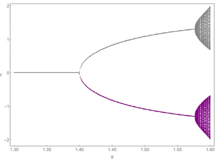
Figure 1: Bifurcation diagram for parameter

= 0.1,

= 0.8,

= 0.5,

= 1,

= 3.5 and 1.3

1.6.

3.3. Numerical illustration

To illustrate our analytical results, we set r = 0.1, v = 0.8, µ = 0.5, aσ

= 1 and β = 3.5 and show in Figure 1 the dynamical behavior of our deterministic model for increasing values of g. As can be seen, the fundamental steady state is stable for g <

2(r + 1) − v = 1.4. At g = 1.4, x

= 0 becomes unstable and two additional steady states emerge. For 1.4 < g < 1.58, our dynamical system may converge to the positive or to the negative non-fundamental steady state. As g increases further, the two non- fundamental steady states also become destabilized and quasi-periodic dynamics arises, as illustrated in Figure 2.

Figure 2 shows the dynamics of our deterministic model for g = 1.6. While the first two panels show time series of price deviations and differences in fractions, the third panel illustrates the attractors in the phase space.

It can be seen from the top panel that prices either cycle around the positive or around the negative unstable non-

8

Note that the eigenvalues of (37) can now be computed and are given by

=

= 0.988 + 0.289i and

= 0.988

0.289i. Since

= 1.06, the complex eigenvalues have just crossed the unit circle and Figure 2 illustrates a situation shortly after the Neimark-Sacker bifurcation.

16

0 100 200 300 400 500 -2

-1 0 1 2

time xt

0 100 200 300 400 500

0.0 0.2 0.4 0.6 0.8 1.0

time mt

-2 -1 0 1 2

0.0 0.2 0.4 0.6 0.8 1.0

x_t mt

Figure 2: Dynamics of our deterministic skeleton for

= 1.6. The first two panels illustrate the evolution of price deviations and differences in fractions for 500 periods, while the third panel shows phase plots in the (x

,

) plane. Parameters are

= 0.1,

= 0.8,

= 0.5,

= 1 and

= 3.5.

fundamental steady state, given by x

= 1.35 and x

= −1.35. The second panel shows the corresponding time series of the difference in fractions. Note that m

= 0.25 and that only one line is visible as the two time series overlap. The attractors plotted in the third panel also reveal that there are coexisting invariant circles around each of the two unstable non-fundamental steady states. However, if g is increased further, the dynamics quickly explodes and prices diverge to infinity.

17

4. Stochastic dynamics

Since our model is able to explain the stylized facts of stock markets, we begin this section by briefly reviewing some of those statistical properties. Furthermore, we introduce some summary statistics to measure the stylized facts we seek to match. In Section 4.2., we report our estimation results and discuss the performance of our model. In Section 4.3., we show a snapshot of our dynamics and explain how the model functions.

4.1. Stylized facts of stock markets

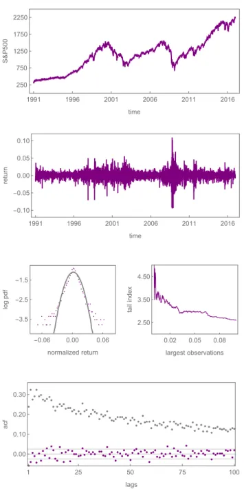
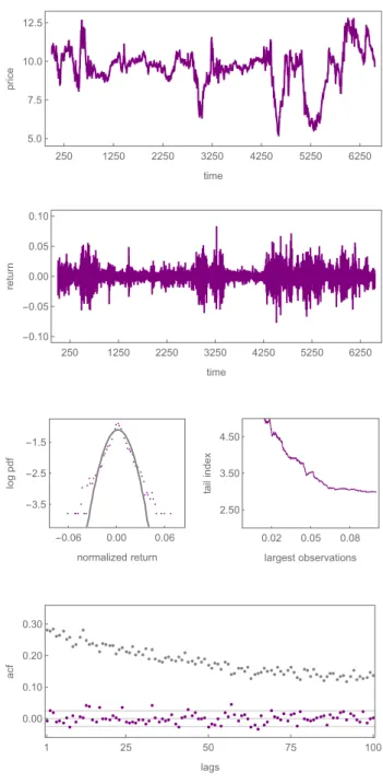
As is well known, the dynamics of stock markets is characterized by (i) bubbles and crashes, (ii) excess volatility, (iii) fat-tailed return distributions, (iv) serially uncorre- lated returns and (v) volatility clustering. Statistical properties of financial markets are surveyed, for instance, by Mantegna and Stanley (2000), Cont (2001), Lux and Ausloos (2002) and Lux (2009). To illustrate these five universal features, we use a time series of the S&P500 stock market index that runs from January 1, 1991 to December 31, 2016 containing 6550 daily observations and show the dynamics in Figure 3. Moreover, we quantify these features by a number of summary statistics, i.e. “moments”, which we present in Table 1.

In the top panel of Figure 3, we depict the daily evolution of the S&P500 between 1991 and 2016. As can be seen, stock prices show strong price appreciations as well as severe crashes. The corresponding return time series is plotted in the second panel.

It reveals that stock prices fluctuate strongly and that extreme price changes of up to 11 percent exist. To measure overall volatility, we compute the standard deviation of returns and obtain a value of V = 1.13 percent per day. The left panel of the third row compares the log probability density functions of normalized returns (purple) and standard normally distributed returns (gray). The distribution of empirical returns ob- viously possesses a higher concentration around the mean, thinner shoulders and again more probability mass in the tails than a normal distribution with identical mean and standard deviation. Since we also want to quantify the fat-tail property, we use the Hill tail index estimator (Hill 1975) and plot it as a function of the largest returns (in percent) on the right-hand side. Note that lower values for the tail index imply fatter tails. For instance, estimates on the largest 5 percent of the observations yield a tail

18

1991 1996 2001 2006 2011 2016 1750

2250

1250 750 250

time

S&P500

1991 1996 2001 2006 2011 2016

0.00 0.05

-0.05 -0.10 0.10

time

return

-0.06 0.00 0.06 -3.5

-1.5 -2.5

normalized return

logpdf

0.02 0.05 0.08 2.50

3.50 4.50

largest observations

tailindex

1 25 50 75 100

0.00 0.10 0.20 0.30

lags

acf

Figure 3: The dynamics of the S&P500. The panels show, from top to bottom, the evolution of the S&P500 between 1991 and 2016, the corresponding returns, the log probability density functions of normalized returns (purple) and standard normally distributed returns (gray), the Hill tail index estimator as a function of the largest returns and the autocorrelation functions of raw returns (purple) and absolute returns (gray), respectively.

19

index of 2.99. However, when we compute the Hill tail index at the 5 percent level for normally distributed returns with T = 6550 and identical mean and standard deviation, we obtain a value of 6.49.

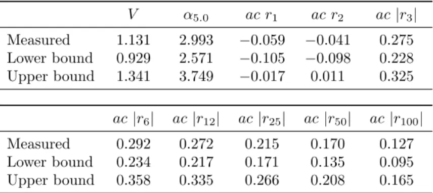
V α

ac r

ac r

ac |r

| Measured 1.131 2.993 −0.059 −0.041 0.275 Lower bound 0.929 2.571 −0.105 −0.098 0.228 Upper bound 1.341 3.749 −0.017 0.011 0.325 ac |r

| ac |r

| ac |r

| ac |r

| ac |r

|

Measured 0.292 0.272 0.215 0.170 0.127

Lower bound 0.234 0.217 0.171 0.135 0.095 Upper bound 0.358 0.335 0.266 0.208 0.165

Table 1: Moments of the S&P500. The first lines contains estimates of the returns’ standard deviation

, the tail index

, the autocorrelation coefficients of raw returns

for lags 1 and 2, and the autocorrelation coefficients of absolute returns

for lags

25, 50,100}. The second and third lines show the lower and upper boundaries of the 95% confidence intervals around the summary statistics that are reported in the first lines. Estimates are based on a time series ranging from January 1, 1991 to December 31, 2016 that contains 6550 daily observations.

In the bottom panel of Figure 3, we show the autocorrelation functions of raw (purple) and absolute (gray) returns for the first 100 lags. The gray lines represent the 95 percent confidence bands. As the autocorrelation of raw returns is insignificant for almost all lags, it follows that the evolution of the S&P500 is close to a random walk. In contrast, absolute returns reveal autocorrelation coefficients that are highly significant for more than 100 lags, which implies a temporal persistence in volatility. It also becomes clear from the second panel of Figure 3 that periods of high volatility alternate with periods of low volatility. To quantify the absence of autocorrelation in raw returns and the long memory in absolute returns, we choose to estimate the autocorrelation coefficients of raw returns for lags 1 and 2, and the autocorrelation coefficients of absolute returns for lags 3, 6, 12, 25, 50 and 100. These summary statistics are presented together with the two described above in the first lines of Table 1.

In the second and third lines of Table 1, we report for all ten moments the lower and upper boundaries of the 95 percent confidence intervals of their bootstrapped frequency distributions. Due to the long-range dependence in the return time series, we follow

20

Winker et al. (2007) and use a block bootstrap to compute the frequency distributions of the returns’ standard deviation and the tail index. To this end, we subdivide the time series of the S&P500 into 26 blocks with 250 daily observations each, construct a new time series from 26 random draws (with replacement) and estimate the values of V and α

from this new block bootstrapped time series. By repeating this 5000 times, we obtain the frequency distributions of the two statistics from which the lower and upper boundaries of the 95 percent confidence intervals can be computed. For the other distributions, however, we choose another bootstrap approach. Franke and Westerhoff (2016) highlight the fact that the long-range dependence in the return time series is al- ways interrupted when two non-adjacent blocks are pasted; they suggest sampling single days together with the past data points required to compute lagged autocorrelations.

Following their argument, we randomly draw 6550 observations with their consecutive data points from the S&P500 time series, compute the lagged autocorrelations, repeat this 5000 times and obtain their distributions.

4.2. Estimation and model performance

Recall that the summary statistics (moments) were introduced to quantify the stylized facts we seek to match. Of course, the simulated moments should be as close as possible to the empirical moments. To this end, we employ the method of simulated moments to estimate our model. For pioneering contributions in this direction, see, for instance, Gilli and Winker (2003), Winker et al. (2007) or Franke (2009). As in Franke and Westerhoff (2012), we use the concept of a joint moment coverage ratio and aim to find the parameter setting that maximizes the fraction of simulation runs for which our simulated moments jointly fall into the 95 percent confidence intervals of their empirical counterparts. To be more precise, we count the number of simulation runs for which all ten moments are contained in the empirical intervals and define the corresponding percentage as the joint moment coverage ratio. The estimation then searches for the parameter setting that maximizes the J M CR score.

However, not all of our model parameters are included in our estimation procedure.

For instance, the value for the interest rate of the risk-free asset can be derived from empirical data. Since the current annual percentage rate is about 0.05, we obtain r = 0.0002 for the daily rate of return. Moreover, the dynamics of our model does not

21

depend on the level of the fundamental value, which is why we set p

= 10, implying that ¯ y = 0.002. To further reduce the number of parameters, we fix N = 300 and set aσ

= 1 as in Brock and Hommes (1998). We also make the simplifying assumption that the correlations of technical and fundamental random trading signals are equal, i.e.

ρ

= ρ

. Hence, there remain seven model parameters for which the maximization of the joint moment coverage ratio yields the following results:

g = 1.001, v = 0.989, σ

= 0.0265, σ

= 0.004607, ρ

= ρ

= 0.78, β = 1550 and µ = 0.992.

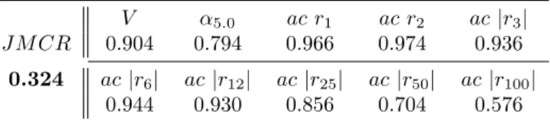
The corresponding value of the J M CR is given by 0.324, i.e. in 32.4 percent of the simulation runs all of our simulated moments drop in their empirical intervals. Given that our objective function is based on the joint matching of ten different moments, such a ratio may be deemed as quite remarkable.

V α

ac r

ac r

ac |r

| J M CR 0.904 0.794 0.966 0.974 0.936

0.324 ac |r

| ac |r

| ac |r

| ac |r

| ac |r

| 0.944 0.930 0.856 0.704 0.576

Table 2: Performance of the model. The table shows the joint moment coverage ratio (J M CR) and the fractions of the individual moments’ matching. Estimations are based on 500 simulation runs with 6550 observations each. Parameters are

= 0.0002,

= 10, ¯

= 0.002,

= 1,

= 300,

= 1.001,

= 0.989,

= 0.004607,

= 0.0265,

=

= 0.78,

= 1550 and

= 0.992.

In Table 2, we show how well our model matches the ten individual moments. For instance, the volatility and the tail index fall in 90.4 percent and 79.4 percent of cases in the 95 percent confidence intervals of their empirical counterparts. The scores are even better for the autocorrelation coefficients of raw returns at lags 1 and 2.

These are given by 96.6 and 97.4 percent, respectively. As can be seen, the model’s ability to generate persistence in volatility is also very good for lags 3, 6, 12 and 25. For higher

9

Note that the empirical intervals of the raw returns’ autocorrelations are centered around

=

−0.059 andac r2

=

dictability, we adjusted the empirical intervals of the two summary statistics by setting their lower and upper boundaries to

almost equally sized as those computed from the bootstrapped distributions.

22

lags, however, autocorrelations of absolute returns are slightly underestimated in some of the simulation runs, which is why we obtain lower scores for lags 50 and 100. Note that we also computed the average moment matching score for this parameter setting and obtained an astounding value of 85.8 percent, i.e. on average, we match 85.8 percent of the empirical moments in a simulation run.

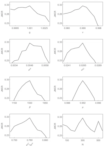
Note that our model parameters were identified by a multi-dimensional grid search in a predefined parameter space. Hence, we cannot rule out the existence of better performing parameter settings. However, any change in one of our estimated model parameters would result in a lower J M CR score, implying that we have found at least a local maximimum of the joint moment coverage ratio. To visualize this, we show in Figure 4 how the model performance depends on our model parameters. For instance, the first panel reveals that the J M CR score decreases if we deviate from g = 1.001.

Obviously, this is also true for v = 0.989, σ

= 0.004607, σ

= 0.0265, β = 1550, µ = 0.992 and ρ

= ρ

= 0.78.

The last panel shows how the number of speculators influences our model performance. Recall that parameter N was not included in our estimation procedure and that we optimized our parameter setting for N = 300. But, as one can see, our model also generates high J M CR scores for other values of N .

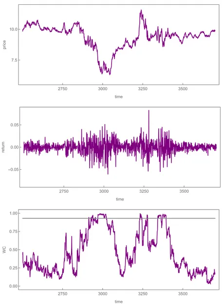
To illustrate the performance of our model, we depict a representative simulation run with 6550 observations in Figure 5. Since we want to compare our model dynamics directly with the dynamics of the S&P500, we use the same design as in Figure 3. Thus, the first panel shows the evolution of prices in the time domain. Apparently, the price of the risky asset fluctuates erratically around its fundamental value p

= 10 and there are a number of periods in which prices either appreciate or depreciate strongly. Hence, our simulated price dynamics can also be characterized by bubbles and crashes. However, there is no long-run upward trend in prices since we assume that the fundamental value is constant. The second panel shows the corresponding return time series and reveals that price volatility is high. There are extreme price changes of up to 8.4 percent and the standard deviation of our simulated returns is given by 1.2 percent, i.e. our model resembles the overall volatility of the S&P500 quite well. From the comparison of the log

10

Note that our estimation results are in line with the empirical evidence reported in the introduction.

While agents’ forecasts are heterogeneous, their expectations are also correlated to some degree.

23

1.001

0.9995 1.0025

0.23 0.33

0.28

g

JMCR

0.989

0.980 0.998

0.23 0.33

0.28

v

JMCR

0.0046

0.0034 0.0058

0.23 0.33

0.28

σ^F

JMCR

0.0265

0.0241 0.0289

0.23 0.33

0.28

σ^C

JMCR

1150 1550 1950

0.23 0.33

0.28

β

JMCR

0.988 0.992 0.996

0.23 0.33

0.28

μ

JMCR

0.780

0.700 0.860

0.23 0.33

0.28

ρ^C=ρ^F

JMCR

100 300 500

0.23 0.33

0.28

N

JMCR

Figure 4: Parameters’ impact on the model’s performance. The panels reveal how the

score depends on parameters

,

,

=

and

is always based on 500 simulation runs.

probability density functions of normalized (purple) and standard normally distributed (gray) returns, exhibited in the left panel of the third row, it becomes evident that our model also gives rise to fat tails. As can be seen, extreme returns occur more frequently than in the case of a normal distribution. This is also confirmed by estimates of the Hill tail index. In the right panel of the third row it can be observed, for instance, that

24

250 1250 2250 3250 4250 5250 6250 5.0

7.5 10.0 12.5

time

price

250 1250 2250 3250 4250 5250 6250

0.00 0.05

-0.05 -0.10 0.10

time

return

-0.06 0.00 0.06 -3.5

-1.5 -2.5

normalized return

logpdf

0.02 0.05 0.08 2.50

3.50 4.50

largest observations

tailindex

1 25 50 75 100

0.00 0.10 0.20 0.30

lags

acf

Figure 5: The dynamics of the model. The panels show, from top to bottom, the evolution of the price, the returns, the log probability density functions of normalized returns (purple) and standard normally distributed returns (gray), the Hill tail index estimator as a function of the largest returns and the autocorrelation functions of raw returns (purple) and absolute returns (gray), respectively. The simulation run is based on 6550 observations.

25