SFB 649 Discussion Paper 2012-022
Assessing the Anchoring of Inflation Expectations
Till Strohsal*
Lars Winkelmann*
* Freie Universität Berlin, Germany
This research was supported by the Deutsche
Forschungsgemeinschaft through the SFB 649 "Economic Risk".
http://sfb649.wiwi.hu-berlin.de ISSN 1860-5664
S FB
6 4 9
E C O N O M I C
R I S K
B E R L I N
Assessing the Anchoring of Inflation Expectations
Till Strohsal and
Lars Winkelmann Freie Universität Berlin This version: February 24, 2012
Abstract
This paper proposes an ESTAR modeling framework to analyze the an- choring of inflation expectations. Anchoring criteria are empirical es- timates of a market implied inflation target as well as the strength of the anchor that holds expectations at the target. Results from daily financial market expectations in the United States, European Monetary Union, United Kingdom and Sweden indicate: First, shorter-term ex- pectations are better anchored than longer-term expectations. Second, expectations are best anchored in the EU, followed by US, Sweden and UK. Third, during the crisis market implied targets mostly decline while the strength of the anchor remains mostly unaffected.
Keywords: Monetary policy, anchoring, inflation expectations, break even inflation rates, ESTAR model.
JEL classification: E52, E58, C32
We thank Jörg Breitung, Ralf Brüggemann, Enzo Weber, Jürgen Wolters and especially Dieter Nautz for valuable discussions, comments, and suggestions. Financial support by the Deutsche Forschungsgemeinschaft (DFG) through CRC 649 “Economic Risk" is gratefully acknowledged.
Freie Universität Berlin, School of Business and Economics, Boltzmannstrasse 20, 14195 Berlin, Germany. E-mail: till.strohsal@fu-berlin.de; lars.winkelmann@fu-berlin.de.
1 Introduction
Expectations play a key role in the conduct of modern monetary policy. In particular the New-Keynesian Phillips curve stresses the importance of inflation expectations for the rate of actual inflation. Central banks’ ability to achieve price stability is thus directly linked to its ability to anchor inflation expectations at their target.
Consequently, major central banks like the Federal Reserve, the Bank of England and the European Central Bank monitor inflation expectations as an indicator of in- flation pressure. The quote "inflation expectations are well-anchored" is a frequently used phrase in press conferences and monetary policy reports. Yet, in spite of their prominent role for monetary policy, inflation expectations are still under-researched, see Bernanke (2007). In particular, it is not clear how the degree of anchoring of inflation expectations should be defined and measured empirically.
In monetary policy practice it is often argued that inflation expectations are well- anchored if their distance to a more or less explicit inflation target is sufficiently small, see BoE (2010, p. 36) and ECB (2011, p. 32). More sophistically, the em- pirical literature employs news regressions and a pass through criterion. The news regression approach exploits the idea that anchored inflation expectations should be insensitive to economic news, compare Levin et al. (2004) and Gürkaynak et al.
(2010b). Similarly, the pass through criterion of Jochmann et al. (2010) and Gefang et al. (2011) defines inflation expectations as anchored if long-term expectations do not respond to changes in short-term expectations. In both approaches, the attention is restricted to the first differences of the inflation expectations measure.
In the present paper, we argue that first differencing leads to a loss of valuable information and imposes implausible dynamics of inflation expectations. In fact, a regression in first differences implies a unit root for the level of expected inflation, i.e. shocks to the level never die out. However, such an extreme persistence appears hardly compatible with the idea of anchored expectations. Moreover, within a first difference regression any information about the level of expected inflation is lost.
Even if the central bank does not announce an explicit inflation target, the level of inflation expectations should be of crucial importance.
For these reasons, we propose to model inflation expectations as an exponential smooth transition autoregressive (ESTAR) process. Nobay et al. (2010) recently showed that the ESTAR model captures the dynamics of the actual rate of inflation
remarkably well.1 As a natural extension, we apply this model to inflation expec- tations data. The distinguishing feature of the ESTAR approach is given by its flexible dynamics. On the one hand, the model allows for the locally high persis- tence typically observed in inflation data, while on the other hand it implies global stationarity, i.e. shocks die out eventually.
In our context, the ESTAR approach assumes that inflation expectations should ultimately return to some long-run equilibrium value or anchor. This value will be interpreted as the market implied inflation target, which may well deviate from the officially announced inflation target of the central bank. The transition speed within the exponential function describes how fast the reversion to the implied target takes place and therefore provides a natural parameter to measure thestrengthof the anchor. The transition function of the ESTAR model implies an increasing incentive to revise expectations the further they deviate from the market implied target.
These characteristics appear suitable and also intuitive in view of anchored inflation expectations. In our empirical excercise economic news variables are included as controls. Therefore, our approach nests the news regression as a limiting case.
We investigate the degree of anchoring of inflation expectations in the United States (US), the European Monetary Union (EU), United Kingdom (UK) and Sweden (SW). The expectations measure under consideration is the so called break even inflation (BEI) rate that is the most prominent measure of inflation expectations within the news regression and the pass through literature. BEI rates can be de- rived from nominal and real government bond yields, i.e. inflation-indexed bonds.
Although the countries under investigation have highly liquid nominal and real bond markets, constant maturity yields of real bonds are usually not readily available. As an exception, constant maturity series of US TIPS are provided by Gürkaynak et al. (2010a). However, in order to construct a homogenous dataset for our cross country study, we closely follow the methodology of Gürkaynak et al. (2010a) and estimate standard Nelson-Siegel-Svensson (Nelson and Siegel 1987, Svensson 1996) yield curves of nominal and real bond yields.
Our results show that the degree of anchoring of inflation expectations varies sub- stantially across countries and expectations horizons. We find that shorter-term ex- pectations are stronger anchored than longer-term, meaning that shocks of a given
1The ESTAR approach is also used to model the dynamics of other macroeconomic time series as, for instance, exchange rates (Kilian and Taylor 2003).
magnitude die out quicker in shorter-term expectations. Among the four countries, the anchoring of expectations is strongest in the EU attended by an implied target close to the ECB’s implied inflation target of 2%. In contrast, UK inflation ex- pectations exhibit the weakest degree of anchoring reflecting very high persistence.
This is accompanied by a high market implied target of up to 4.3%. In view of inflation expectations in the US, a comparison of a pre- and post-Lehman period shows that the strength of the anchor of shorter-term expectations decreases, while for longer-term it increases.
The remainder of the paper is structured as follows. Section 2 introduces the anchor- ing criterion based on the ESTAR model. The measure of inflation expectations, i.e.
BEI rates, are introduced in Section 3. Furthermore, Section 3 comprises a prelimi- nary data analysis with descriptive statistics and linearity tests. Estimation results including an impulse response analysis and a comparison to the news regression literature are discussed in Section 4. Section 5 concludes.
2 The anchoring criterion
The degree of anchoring is analyzed by means of an exponential smooth transition autoregressive (ESTAR) model.2 The adequacy of the ESTAR specification in the present context of inflation expectations is evidenced by linearity tests as to be shown in the next section. The ESTAR model is given by:
yt=c+ exp−γ(yt−1 −c)2
p
X
i=1
αiyt−i−c
!
+βXt+εt , (1)
where yt represents the measure of inflation expectations, i.e. the BEI rate, and c is a constant. The sum of autoregressive parameters is restricted to Ppi=1αi = 1 and Xt constitutes a vector of economic news variables, withβ as the corresponding coefficient vector and εtas a zero mean white noise process. The dynamics ofyt are determined by the exponential smooth transition function exp(−γ(yt−1−c)2) which is the source of non-linearity in this model. The transition function is bounded between zero and one and depends on the transition variable yt−1, a smoothness
2We consider a restricted version, that is applied prominently in the literature on purchasing power parity and to model the actual rate of inflation, see among others Kilian and Taylor (2003) and Nobay et al. (2010), respectively.
parameter γ > 0 and a location parameter c. Given the restriction of the sum of autoregressive parameters, model (1) behaves locally like a random walk if the lagged expectations measure yt−1 equals c. Ifyt−1 departs fromc, the process is stationary and therefore mean reverting. As shown in Kapetanios et al. (2003), despite its local non-stationarity, the ESTAR model is globally stationary. The degree of mean reversion at time t depends on the squared difference between yt−1 and c.
In economic terms, ccan be interpreted as an equilibrium value that consists of the market implied inflation target and an inflation risk premium. If the BEI rate was close to its equilibrium value cin the last period, a shock to inflation expectations has a long lasting impact. However, when shocks drive the BEI rate away from its equilibrium value, the anchor comes into play and pulls expectations back to the equilibrium. Due to the non-linearity of the model, the strength of the anchor increases in the distance to the equilibrium value, i.e. the larger the gap between yt−1 and cthe stronger the mean reversion. The parameter γ controls the shape of the exponential function and therefore the transition speed towards c. The largerγ, the larger the slope of the exponential function around cand, thus, the stronger the attraction of the market implied inflation target. Given estimates of the ESTAR model, we interpret expectations as better anchored the larger the transition speed γ and the closer the equilibrium value c to the central bank’s inflation target.
Apart from the non-linear dynamics, (1) includes potential driving forces behind the BEI rates. The β coefficient vector indicates important macroeconomic and mon- etary variables that cause market participants to revise their expectations. Hence, estimation results can be interpreted with respect to the sensitivity to news argu- ment as well. Regarding our econometric approach, the crucial difference to the standard news regression is that model (1) allows the expectations measure to mean revert. In fact, the news regression given by
∆yt =βXt+εt, (2)
implies a unit root in the level of yt. The ESTAR extension of (2) mitigates this assumption. Yet, due to the local random walk behavior, for p = 1 and expecta- tions at their equilibrium value, yt−1 = c, (1) collapses to the news regression (2).
Moreover, model (1) nests the news regression for the special case p= 1 and γ = 0.
Linearity tests carried out in the next section provide evidence on the adequacy of ESTAR non-linearities against the unit root assumption.
3 Break even inflation rates
The expectations data is extracted from nominal and real government bond yields.
According to the Fisher equation, the spread between nominal and real yields gives a measure of inflation expectations, i.e. the break even inflation (BEI) rate.3 Since the holder of a nominal bond faces inflation risk4 against which an investor holding a real bond is protected, break even rates are not a pure measure of inflation expectations.
Thus, break even inflation rates consist of inflation expectations and an inflation risk premium. In order to disentangle the two components, affine term structure models of e.g. Adrian and Wu (2009) and Christensen et al. (2010) are available.
However, such a filtered inflation measure strongly depends on the choice of the model and, of course, is subject to estimation uncertainty. Furthermore, given our interest in the anchoring of inflation expectations, including the premium as a part of the relevant variable, provides important information. Precisely, a central bank that aims to stabilize inflation expectations should also aim to minimize the inflation risk premium. Therefore, we rely on BEI rates to evaluate the anchoring of inflation expectations.
Countries under investigation are the United States (US), European Monetary Union (EU), United Kingdom (UK) and Sweden (SW). The country selection is consistent with the former anchoring literature and is also narrowed by data availability. We investigate daily data in the time span from January 2004 to February 2011. By starting in 2004 we ensure that the countries have highly liquid nominal and real bond markets across a wide range of maturities. Since BEI rates are not readily available for most of the countries, we follow the methodology of Gürkaynak et al.
(2007) and Gürkaynak et al. (2010b) and estimate nominal and real Nelson-Siegel- Svensson yield curves to finally obtain coherent term structures of BEI rates across the different countries under investigation.5 The inflation expectations measure is the one-year forward break even inflation rate for two different time horizons. The five-year horizon reflects todays expectations about inflation (and the risk premium)
3Also known as inflation compensation.
4I.e. the uncertainty about an unexpected rise in the actual inflation rate over the holding period.
5By building a coherent dataset we are intended to minimize the risk of distortions induced by using different data sources that rely on different methodologies. For instance, the FED uses the Nelson- Siegel approach while the Bank of England applies a spline method; the criteria for choosing the specific bonds also differ between different data sources. For details on our methodology see Appendix A.
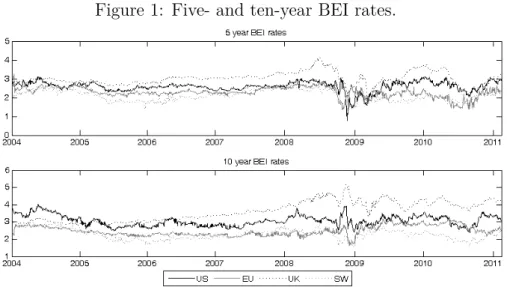
Figure 1: Five- and ten-year BEI rates.
Note: Calculated via nominal and real forward rates from Nelson-Siegel-Svensson yield curves. The five-year rate reflects expectations in five years for one year, the ten-year rate expectations in ten years for one year.
in five years for one year. The one-year forward in five years captures central banks ability to anchor inflation expectations within the often defined policy horizon of three up to five years. Beside the five-year horizon we compute the ten-year horizon, i.e. todays expectations from year ten to year eleven. This allows us to contrast the results with the existing literature, since Gürkaynak et al. (2010a) and Beechey et al. (2011) use a ten-year horizon to explore the insensitivity to news criterion.
Figure 1 depicts the five (upper part) and ten (lower part) year expectation horizons for the different countries. The figure reflects that market participants expect infla- tion around two and three percentage points. Revisions of expectations are rather small on a day to day basis such that the depicted series behave very persistently.
Since the impact of the global financial crisis is clearly visible, we consider a pre- crisis and a crisis period. We follow a standard treatment of dating the crisis by defining the bankruptcy of Lehman Brothers on September 15th 2008 as its starting point. Note, that our crisis period lasts until the end of the sample in 2011, thus, incorporates the sovereign debt crisis as well.
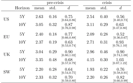
Table 1 confirms the indications of Figure 1. Break even rates across the different countries and time horizons are on average well-above the two percentage mark.6
6The two percentage mark serves as an inflation target in the EU, UK and Sweden.
Table 1: Descriptive statistics before and after Lehman’s bankruptcy.
pre-crisis crisis
Horizon mean std. d mean std. d
US 5Y 2.63 0.16 0.75
[0.64,0.86] 2.54 0.40 0.56
[0.40,0.73]
10Y 3.05 0.32 0.87
[0.76,0.98] 3.11 0.29 0.63
[0.47,0.80]
EU 5Y 2.40 0.18 0.77
[0.66,0.88] 2.09 0.28 0.52
[0.36,0.67]
10Y 2.37 0.19 0.63
[0.53,0.74] 2.71 0.31 0.93
[0.76,1.10]
UK 5Y 3.04 0.29 0.90
[0.80,1.02] 2.96 0.46 0.90
[0.74,1.08]
10Y 3.35 0.48 0.68
[0.57,0.79] 4.15 0.30 1.03
[0.87,1.22]
SW 5Y 2.20 0.28 0.64
[0.54,0.75] 1.93 0.22 0.76
[0.58,0.91]
10Y 2.33 0.32 0.70
[0.59,0.80] 2.20 0.26 0.82
[0.66,0.99]
Notes: Mean and standard deviation in percentage point. d stands for the order of fractional integration estimated by the Local Whittle Wavelet estimator. Pre-crisis sample Jan 2004 - Sep 2008 (∼1200 obs.), crisis period Sep 2008 - Feb 2011 (∼630 obs.).
For most countries the mean and the standard deviation are larger for the ten-year horizon than for the five-year horizon. A clear pattern of how the crisis affects the expectations measure is not visible. The persistence of the series, evidenced by the order of fractional integration, lies within the interval (0.5,1), where processes are still mean reverting but display an unbounded variance. Time series with such an integration order are non-stationary. The order of fractional integration within (0.5,1) can be taken as a first indication of non-linearities in the true underlying processes, see Kruse and Sibbertsen (2011).
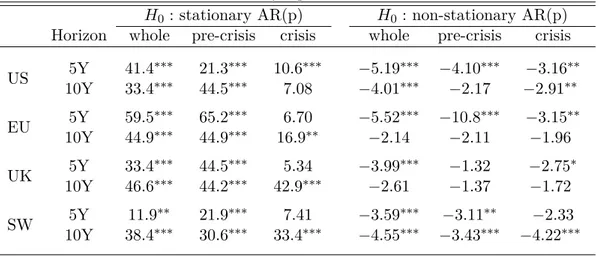
For specification of the ESTAR model, we perform two different types of linearity tests. Both approximate the exponential function in (1) around γ = 0 to obtain an auxiliary regression. The t-test of Kapetanios et al. (2003) (KSS) tests the null of a linear non-stationary autoregressive process against ESTAR non-linearities. We also run the LM test of Saikkonen and Luukkonen (1988) and Teräsvirta (1994) to test the null of a linear stationary autoregressive process against ESTAR non- linearities. We carry out both tests since conventional autoregressive models are close to non-stationarity such that standard unit root tests show conflicting test
Table 2: Linearity against ESTAR tests.
H0: stationary AR(p) H0: non-stationary AR(p) Horizon whole pre-crisis crisis whole pre-crisis crisis US 5Y 41.4∗∗∗ 21.3∗∗∗ 10.6∗∗∗ −5.19∗∗∗ −4.10∗∗∗ −3.16∗∗
10Y 33.4∗∗∗ 44.5∗∗∗ 7.08 −4.01∗∗∗ −2.17 −2.91∗∗
EU 5Y 59.5∗∗∗ 65.2∗∗∗ 6.70 −5.52∗∗∗ −10.8∗∗∗ −3.15∗∗
10Y 44.9∗∗∗ 44.9∗∗∗ 16.9∗∗ −2.14 −2.11 −1.96 UK 5Y 33.4∗∗∗ 44.5∗∗∗ 5.34 −3.99∗∗∗ −1.32 −2.75∗
10Y 46.6∗∗∗ 44.2∗∗∗ 42.9∗∗∗ −2.61 −1.37 −1.72 SW 5Y 11.9∗∗ 21.9∗∗∗ 7.41 −3.59∗∗∗ −3.11∗∗ −2.33
10Y 38.4∗∗∗ 30.6∗∗∗ 33.4∗∗∗ −4.55∗∗∗ −3.43∗∗∗ −4.22∗∗∗
Notes: Test statistics of the LM test with the null hypothesis of a stationary autore- gressive process and KSS with the null of a non-stationary autoregressive process.
Lag length chosen such that residuals are free from significant autocorrelation. ∗ indicates the rejection of the respective null hypothesis at the 10%,∗∗at the 5% and
∗∗∗ at the 1% level. Sample: whole: Jan 2004 - Feb 2011; pre-crisis: Jan 2004 - Sep 2008; crisis: Sep 2008 - Feb 2011.
results.
Table 2 shows the results of the two linearity tests. The LM test rejects the null across all countries and almost all sample periods. For a given country, expectation horizon and sample period, at least one of the two tests rejects the null in favor of the ESTAR model.7 Consequently, we interpret these results as extensive evidence that the true underlying processes can be well-approximated by an ESTAR model.
4 Results
4.1 ESTAR estimation
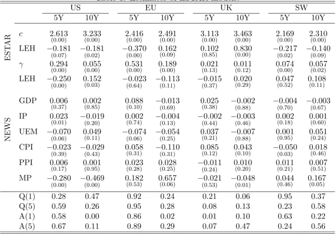
As presented in the previous section, we observe strong evidence that BEI rates follow an ESTAR process. Results shown in Table 3 are obtained from maximum
7The exception to this is the Swedish five-year BEI rate in the crisis sample. However, the test statistic of 7.41 corresponds to ap-value of 0.11 and the KSS test statistic of−2.33 falls above the 10% level of −2.66. Even though at the 10% level tests fail to reject the null, they point in the non-linear direction. In general, due to the sample split, linearity tests tendencially suffer from low power which may in part explain the failure of rejecting the null in a few cases.
likelihood estimation of equation (1). Since the financial market data reveals the typical conditional heteroskedastic pattern, the errors are specified as GARCH(1,1).
The lag lengthpvaries between 1 and 4 and is determined by standard autocorrela- tion tests. TheQ-statisticsQ(1) andQ(5) in the lower part of Table 3 illustrate that no significant autocorrelation is left in the residuals. ARCH LM test results analo- gously reflect that, apart from a few exceptions, the parsimonious GARCH(1,1) is sufficient to capture the conditional heteroskedasticity. Confirming the results from the LM and KSS specification tests, coefficient estimates of c and γ are significant for all countries but the UK.8
Since the ongoing financial crisis potentially changes the degree of anchoring, we account for parameter shifts within our ESTAR specification (1). In particular, a Lehman step dummy LEH that takes the value one from 9/15/2008 until the end of the sample captures breaks in parameter values ofcandγ. Note, that the estimation results of the time series dynamics have proven to be robust against a sample split, i.e. separate estimation of the pre-crisis and crisis sample. Beside analyzing the time series dynamics, we also aim to explore potential sources of shocks that may drive inflation expectations. Therefore, we include news variables as exogenous regressors. News about real economic activity, price developments and monetary policy are taken from Bloomberg’s survey.9 News variables measure the surprise component of each announcement as the difference between the released value and its mean prediction.10
As motivated in Section 2, ESTAR coefficients that reflect the equilibrium value, c, and the transition speed towards the equilibrium,γ, are taken to evaluate the degree of anchoring. Since Christensen et al. (2010) find for US BEI rates that the inflation risk premium is on average close to zero, estimates of the equilibrium values should be close to the market implied inflation target. Results on the anchoring of inflation expectations are interpreted among three different lines: first, across the different expectation horizons, second, across countries and, third, across the pre-crisis and crisis period.
8However, due to the well-known difficulties to get precise estimates of the transition coefficientγ, thep-values of 0.13 and 0.12 do not strongly contradict the ESTAR specification of the UK BEI rates.
9Bloomberg’s survey is based on a selection of professional economists who submit their forecasts to Bloomberg before or on the Friday prior to the data release, see Appendix B.
10We run the same type of regressions with median expectations. Qualitative results remain the same.
Table 3: Estimates of ESTAR models.
US EU UK SW
5Y 10Y 5Y 10Y 5Y 10Y 5Y 10Y
ESTAR
c 2.613
(0.00) 3.233
(0.00) 2.416
(0.00) 2.491
(0.00) 3.113
(0.00) 3.463
(0.00) 2.169
(0.00) 2.310
(0.00)
LEH −0.181
(0.07)
−0.181
(0.02)
−0.370
(0.00)
0.162
(0.09) 0.102
(0.85) 0.830
(0.00)
−0.217
(0.02)
−0.140
(0.09)
γ 0.294
(0.00) 0.055
(0.00) 0.531
(0.00) 0.189
(0.00) 0.021
(0.13) 0.011
(0.12) 0.074
(0.00) 0.057
(0.02)
LEH −0.250
(0.00)
0.152
(0.03)
−0.023
(0.64)
−0.113
(0.11)
−0.015
(0.37)
0.020
(0.29) 0.047
(0.52) 0.108
(0.11)
NEWS
GDP 0.006
(0.37) 0.002
(0.85) 0.088
(0.10) −0.013
(0.69)
0.025
(0.38) −0.002
(0.88)
−0.004
(0.70)
−0.003
(0.67)
IP 0.023
(0.01) −0.019
(0.20)
0.002
(0.74) −0.004
(0.13)
−0.002
(0.44)
−0.003
(0.46)
0.002
(0.18) 0.001
(0.60)
UEM −0.070
(0.06)
0.049
(0.11) −0.074
(0.06)
−0.054
(0.25)
0.037
(0.21) −0.007
(0.88)
0.001
(0.95) 0.051
(0.24)
CPI −0.023
(0.39)
−0.029
(0.43) 0.058
(0.31) −0.110
(0.31) 0.085
(0.12) 0.043
(0.10) −0.050
(0.03) 0.018
(0.46)
PPI 0.006
(0.17) 0.001
(0.95) 0.023
(0.28) 0.028
(0.25)
−0.011
(0.24)
0.010
(0.20) 0.011
(0.21) 0.007
(0.51)
MP −0.280
(0.00)
−0.469
(0.00) 0.182
(0.53) 0.657
(0.06) −0.021
(0.53)
−0.048
(0.01) 0.044
(0.46) 0.167
(0.05)
Q(1) 0.28 0.47 0.92 0.24 0.21 0.06 0.95 0.37
Q(5) 0.59 0.26 0.95 0.28 0.08 0.13 0.23 0.58
A(1) 0.58 0.00 0.86 0.02 0.01 0.10 0.63 0.22
A(5) 0.67 0.11 0.89 0.29 0.07 0.47 0.24 0.56
Notes: ML estimation results of equation (1): yt=c+cLEH+exp −(γ+γLEH)(yt−1−(c+cLEH))2 (P
iαiyt−i−(c+cLEH))+
βXt+εt. yt := daily BEI rates in the time span Jan 2004 to Feb 2011. LEH:= step dummy that takes the value one from 9/15/2008 till 2/14/2011 and zero elsewhere. BEI rates and macroeconomic news, Xt, in percentage points (news coefficients
10
Beginning with the inner country comparison, evidence points towards a better anchoring of inflation expectations for the five-year horizon than for the ten-year horizon. Equilibrium values across countries are on average around 2.5 percentage points for five-year expectations and close to 3 percentage points for the ten-year expectation horizon. The deviations of the equilibrium values from a target value of two percent can be explained by a positive risk premium and a higher market implied inflation target compared to the central bank’s target. Confirming results of Christensen et al. (2010), the comparison of the five and ten-year horizon indicates, that markets associate longer expectation horizons with higher uncertainty about inflation and, thus, with a larger risk premium. Values of transition speeds point in the same direction. For the five-year expectation horizon, transition speeds are on average 1.5 times larger than for the ten-year horizon. The larger γ indicates that the anchor affects shorter-term expectations stronger than longer-term expectations.
Thus, it is not just the level of the expectations measure which makes shorter expec- tation horizons appear better anchored but also the strength with which the anchor pulls them back to their equilibrium value.
The often defined policy horizon of central banks between three and five years can be taken as a reason for the better anchoring of shorter-term expectations. This reflects, markets expecting a more active role of central banks against medium term inflationary pressure. As a consequence, shocks to longer-term expectations are more persistent.
The cross-country comparison for the market implied targets reveals a clear pattern.
Regardless of the maturity and sample period, inflation expectations in Sweden are anchored around the smallest equilibrium values ranging between 1.94 and 2.31 percent. While the EU has slightly larger equilibrium values (between 2.05 and 2.65 percent), EU BEI rates have the fastest transition speeds and, thus, the strongest anchor. Both, c and γ estimates for the UK data show the worst performance. In particular, during the crisis period UK BEI rates vary around an equilibrium value of 3.11 and 4.29 percent and exhibit by far the smallest transition speed. For a given value of cour point estimates of γ suggest that EU expectations are best anchored followed by US, Sweden and finally UK.
Providing empirical evidence on the question why some countries have better an- chored expectations than others, lies beyond the scope of this paper. However, it appears quite clear that the anchoring order can not simply be explained by dif-
ferences in monetary policy strategies like inflation targeting or the overall degree of transparency. While the Bank of England and the Swedish Riksbank are both inflation targeters and are better ranked in transparency studies such as Dincer and Eichengreen (2007), the ECB and FED have stronger anchors that pull inflation expectations back to their equilibrium.
Since the global financial crisis as well as the subsequent sovereign debt crisis is covered by the sample period, it is interesting to explore potential effects of the crisis period on the anchoring of inflation expectations. P-values corresponding to t-tests of the LEH dummies indicate whether it is likely that a shift occurred at the Lehman crash. Overall, the impact of the crisis does not point in a unique direction.
Equilibrium values of the BEI rates change in all countries significantly. In the US and Sweden c decreases for the five and ten-year expectation horizons, indicating recession concerns and, thus, decreasing inflationary pressure. In contrast, equilib- rium values in the UK rise, reflecting inflationary pressure that potentially results from massive policy interventions and worries about stagflation. In the EU the term structure of BEI rates steepens due to a decreasing shorter-term equilibrium and an increasing longer-term equilibrium. Unlike the equilibrium values, the transition speed in most of the countries does not change significantly. Consequently, the crisis does not affect the strength of the anchors. An exception to this invariance are the five and ten-year expectation horizons in the US. While for the medium term horizon the transition speed decreases, for longer-term horizons it increases. This reflects a growing degree of anchoring for longer-term horizons and a shrinking degree for shorter horizons. All in all, during the crisis period inflation expectations remain well-anchored in all countries.
While time series dynamics determine the degree of anchoring, surprise components of major economic announcements reveal potential sources of shocks that drive ex- pectations away from their equilibrium value. Significant coefficients reported in the lower part of Table 3 indicate news announcements that lead to systematic revi- sions in inflation expectations. In general, we observe only few announcements that move markets’ expectations significantly. For example, news about real economic activity impact the five-year horizons in the US and EU. Given an unexpected, one percentage point increase in the US industrial production (IP) index, the five-year BEI rate increases by 2.3 basis points. In the same vein, inflation expectations decrease around 7 basis points in the US and EU for an unexpected, one percent-
age point increase in the unemployment rate (UEM). Unexpected changes in prices, measured by the consumer price index (CPI) and the producer price index (PPI), are mostly non-significant. Monetary policy (MP), however, shows a significant im- pact in all countries. The strongest response to monetary policy news can be found at the ten-year horizon in the EU. An unexpected one percentage point lower policy rate decreases the expectations measure by 65 basis points. Interestingly, given a smaller increase in the policy rate than expected, inflation expectations in the US and UK rise while expectations in the EU and Sweden fall. These asymmetric re- sponses demonstrate that US and UK markets evaluate such policy moves as being too weak to prevent the actual inflation rate from rising. In contrast, markets in the EU and Sweden adopt central banks’ assessments of lower inflationary pressure.
The different responses may reflect a stronger faith in central banks in the EU and Sweden. This interpretation agrees with findings of our cross-country comparison on the anchoring of inflation expectations.
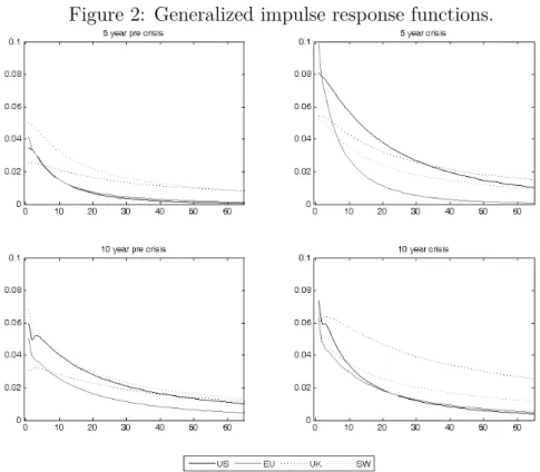
Due to the global stationarity of the ESTAR specification, the effect of a shock of any nature disappears. It is therefore interesting to analyze, in which way and how long a shock affects the expectations measure. The impulse response analysis in the following subsection provides a tool to illustrate the anchoring of inflation expectations.
4.2 Impulse response analysis
In order to support the findings on the anchoring of inflation expectations, we com- pute impulse response functions from the estimated models. Thereby, we intend to emphasize the mean reversion properties of the expectations measure across the different countries and time horizons. Since the impulse response function of a non- linear model depends on the process’ history, the size and sign of the initial shock and on the realizations of future shocks, standard impulse response techniques from linear models are not applicable. Therefore we compute generalized impulse re- sponse functions (GIRFs) as suggested by Koop et al. (1996).11 Given an estimate of an ESTAR process, the GIRF averages over all possible histories and future re- alizations to isolate the effect of the initial shock. We set the size of this impulse equal to plus one residual standard deviation. In order to compare the mean rever-
11See Appendix C, for further details on computational steps.
Figure 2: Generalized impulse response functions.
Note: The magnitudes of the shocks are set to plus one standard deviation of residuals in the respective subsample. Graphs show the initial impact att= 0 and the shock absorption up to three month ahead, i.e. units of x-axes refer to days.
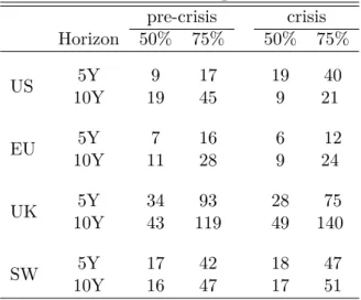
sion properties, we compute X-lives from the different impulse responses. X-lives indicate the number of days an initial shock needs to be absorbed byX percent. We chose to focus on half-lives, i.e. X = 50%, and the absorption time for X = 75%.
Figure 2 depicts the impulse response functions, Table 4 reports theX-lives. Results confirm the findings from the previous subsection. Expectations appear better an- chored for the five-year horizon than for the ten-year horizon. Values of the impulse response functions at time zero, are on average larger for ten-year expectations.
This expresses a smaller noise variance in shorter-term expectations compared to longer-term expectations. X-lives further support the findings of a better anchoring of shorter-term expectations. In comparison to the five-year horizon, a one standard deviation shock to the ten-year horizon needs on average about three weeks longer to be absorbed by 75%. The cross-country comparison confirms that expectations are best anchored in the EU. For example, during the pre-crisis period a one stan-
Table 4: X-life absorption time.
pre-crisis crisis Horizon 50% 75% 50% 75%
US 5Y 9 17 19 40
10Y 19 45 9 21
EU 5Y 7 16 6 12
10Y 11 28 9 24
UK 5Y 34 93 28 75
10Y 43 119 49 140
SW 5Y 17 42 18 47
10Y 16 47 17 51
Notes: Reported values represent the absorption time measured in days for 50% and 75% of the initial shock size of one residual standard deviation.
dard deviation shock to the five-year expectations measure vanishes by 50% after seven days and by 75% after 16 days. In contrast, half-lives of a one standard de- viation shock to UK expectations are in general larger than one month. Regarding the pre-crisis and crisis sample, Figure 2 indicates larger noise variances during the crisis. Due to the anchoring characteristics of ESTAR models, for a given transi- tion speed, γ, larger shocks decay quicker than smaller shocks. Since most of the countries display a non-significant break in the transition speed,X-lives remain con- stant (Sweden) or slightly decrease (EU). The significant breaks in the US transition speeds increase the half life of the five-year horizon from 9 to 19 days while the half life of the ten-year horizon decreases by the same amount.
In sum, the decay of the impulse responses illustrates the main idea of the proposed anchoring criterion, i.e. anchored inflation expectations display stationary character- istics. Given the equilibrium values estimated in the previous subsection, half-lives indicate well-anchored inflation expectations across the different expectation hori- zons, countries and sample periods.
4.3 Comparison to the former anchoring literature
Different anchoring criteria potentially produce different results on the anchoring of inflation expectations. Since the ESTAR model nests the news regression as a
special case, the comparison focuses on the news regression approach.
Results presented in subsection 4.1 show a weaker impact of economic news com- pared to the news regression literature. Especially, results for the ten-year expecta- tion horizon in the US differ from the results presented in Gürkaynak et al. (2010b) and Beechey et al. (2011). While the authors find variables like the GDP and CPI to have a significant effect, monetary policy is the only source of news that affects our ten-year US BEI rate. In the context of the news regression criterion, our results in- dicate well-anchored expectations in all countries under investigation. Consequently, cross-country differences or differences across expectation horizons cannot be found.
One possible explanation for the contrasting results from the news regressions can be attributed to the analysis of different sample periods. According to Beechey and Wright (2009), a more recent sample period implies higher liquidity of real bonds.
The authors show that since 2004 the high liquidity of real bonds in the US allows for immediate adjustments to economic news such that forward BEI rates respond non-significantly.
The news regression literature usually explains different degrees of anchored inflation expectations by differences in monetary policy strategies. Cruijsen and Demertzis (2007) find that expectations are better anchored the more transparent a central bank is. In the same vein, Gürkaynak et al. (2010b) find inflation targeters to bet- ter anchor inflation expectations than non-targeters. As argued in 4.1, the ESTAR criterion does not confirm such explanations. A further difference of the results from news regressions and the ESTAR criterion is revealed by comparing the anchoring of shorter expectation horizons with the anchoring of longer horizons. Referring to impulse responses of the actual rate of inflation within standard macroeconomic models, shorter-term expectations are more sensitive to economic news (shocks) than longer expectation horizons. In that context, Beechey et al. (2011) show empirically that longer expectation horizons are better anchored than shorter expectation hori- zons. Regarding the ESTAR anchoring criterion, we find the exact opposite to hold true. In comparison to longer expectation horizons, shorter-term expectations have a smaller equilibrium value and a faster adjustment speed, thus, appear better anchored.
The comparison shows that conclusions about the anchoring of inflation expectations crucially depend on the way the anchoring criterion is chosen. Consequently, the various characteristics of inflation expectations measures are hardly captured by
one single criterion. This emphasizes the need to consider different approaches to determine the degree of anchoring.
5 Conclusion
Both policy makers and academia increasingly pay attention to the question whether inflation expectations are well-anchored. The prominence of this topic can be at- tributed to standard forward-looking macroeconomic models wherein the anchoring of inflation expectations appears as a necessary condition to stabilize the actual rate of inflation.
In this paper we propose a non-linear time series approach to determine the de- gree of anchoring. Thereby we complement one well-known analytical framework for investigating the anchoring of inflation expectations, namely the news regression, wherein first differences of an expectations measure are regressed on macroeconomic news. We especially relax the implicit unit root assumption of the news regression approach and allow anchored inflation expectations to follow a globally stationary ESTAR process. The generalization permits a shift of the focus from the short run news effect to the long run dynamics of inflation expectations. Model parameters are economically interpretable as a market implied inflation target and the strength of the anchor that drives expectations back to the target. Both parameters deter- mine the degree of anchoring. As a measure of inflation expectations we compute break even inflation (BEI) rates from nominal and inflation-indexed Nelson-Siegel- Svensson yield curves for the US, EU, UK and Sweden. Empirical evidence is based on one-year forward BEI rates with five- and ten-year expectation horizons in the time span 2004 to 2011.
Specification tests confirm that BEI rates are well-described by an ESTAR process.
The ESTAR anchoring criterion provides three main results. First, the market im- plied inflation target around 2.5 percent for shorter-term expectations is around half a percentage point smaller than for longer-term expectations. At the same time, im- pulse responses indicate a much quicker shock absorption of shorter-term BEI rates.
For a 75% shock absorption the difference is roughly three weeks. Consequently, shorter-term inflation expectations appear better anchored than longer-term expec- tations. Second, expectations in the EU are best anchored followed by the US, Sweden and UK. Especially the EU has the fastest adjustment speed with a half
life smaller than two weeks and one of the smallest market implied inflation targets within a range around 2.05 and 2.65 percent. In contrast, long term expectations in the UK are extremely persistent with half-lives of more than one month and an exceptionally high market implied inflation target of up to 4.3 percent. Third, a significant effect of the global financial crisis is only found for the market implied inflation targets. Reflecting recession concerns, inflation pressure in most of the countries declines during the crisis. In contrast, the strength of the anchors are mostly not affected by the crisis.
The news regression literature explains cross-country differences in the anchoring of inflation expectations by differences in the transparency of central banks or by specific policy strategies such as inflation targeting. The present study cannot con- firm these findings. Investigating explanations for these differences constitutes an interesting path for future research. A further aspect of the present paper is given by the analysis of driving forces behind the expectation formation processes. Since our results indicate that major economic news releases have only a marginal impact on expectations, models that reveal structural relations could provide further insights.
For example, cross-country interdependencies such as spillover effects, especially during the economic crisis, may play an important role.
Given central banks’ mandate to stabilize the actual rate of inflation, in all countries under investigation our results support the view of credible policy strategies that anchor inflation expectations. Apart from the UK, the market implied inflation targets are close to the usually imposed inflation targets of 2 percent. Moreover, expectations vary in a stationary manner around these targets. This leads to the conclusion that expectation formation processes are successfully controlled by central banks.
For policy makers our analysis suggests that it is necessary to evaluate the success of the anchoring of inflation expectations with respect to different criteria. We find that conclusions on the anchoring can strongly depend on the way the criterion is chosen. Since our proposed model nests the news regression, it provides an appealing framework to combine the anchoring analysis with respect to time series dynamics as well as the sensitivity to news criterion.
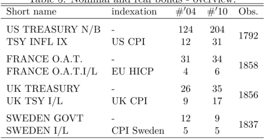
A Term structure estimation
Our data set is based on bond yields downloaded from the Bloomberg database, see the overview in Table 5. We take into account all outstanding, standard government bonds (e.g. no callables) with more than two years time to maturity. Bonds with less than 24 month to maturity are cut out because real bonds’ indexation lags make the yields of these securities erratic, see Gürkaynak et al. (2010a).
Table 5: Nominal and real bonds - overview.
Short name indexation #004 #010 Obs.
US TREASURY N/B - 124 204
TSY INFL IX US CPI 12 31 1792
FRANCE O.A.T. - 31 34
FRANCE O.A.T.I/L EU HICP 4 6 1858
UK TREASURY - 26 35
UK TSY I/L UK CPI 9 17 1856
SWEDEN GOVT - 12 9
SWEDEN I/L CPI Sweden 5 5 1837
Notes: #004, #010 reports the number of outstanding bonds in June 2004 and 2010, Obs. is the number of daily observations within the time span Jan 2004 and Feb.
2011. EU HICP refers to the harmonized index of consumer prices of the European Monetary Union.
For each day, where yields for more than three bonds are available, we follow the approach of Gürkaynk et al. (2007), and estimate constant maturity yields. The standard parametric yield curve specification is based on a functional form that was proposed by Nelson and Siegel (1987) and extended by Svensson (1994):
ˆ
zt(τ) = β1+β2
1−e−λτ1
τ λ1
+β3
1−e−λτ1
τ λ1
−e−λτ1
+β4
1−e−λτ2
τ λ2
−e−λτ2
. (3) The observed zero coupon yield for maturity τ is given by z(τ), whereas the model implied yield is ˆz(τ). We minimize P(ˆz(τ)−z(τ))2 with respect to the parameters β1, β2, β3, β4, λ1 and λ2 by the Differential Evolution approach proposed by Storn and Price (1997). From zero-coupon yield curves, forward rates are derived via
ft(n, m) = 1
m((n+m)ˆzt(n+m)−nˆzt(n)), (4)
whereft(n, m) is the forward rate at timetfor a period ofmyears beginningnyears in the future. The n-year BEI rate reflects today’s expected inflation rate (plus an inflation risk premium) and is given by BEI(n) = ftnom(n, m)−ftreal(n, m).
As documented in Gürkaynak et al. (2010), the FED provides a periodically updated dataset of US BEI(n) (with n = 4, 5 and m = 1) rates at www.federalreserve.gov/
econresdata/researchdata.htm. The correlation to our US BEI(n) rates is well-above 0.9.
B News variables
The news variables are calculated as the difference between the actual and the expected value. The expected value is represented by the mean prediction of the Bloomberg survey of professional economists. Economists are mostly bankers. They submit their forecast before or on Fridays prior to the data release. The actual and forecasted values of the advanced estimate of the gross domestic product (GDP), industrial production (IP), consumer price index (CPI) and the producer price index (PPI) refer to the percentage year on year change. The GDP, IP, CPI and PPI news, consequently measure the difference between the actual and forecasted value in percentage points. The unemployment rate (UMP) and the monetary policy rate (MP) are measured in percent. The respective news variable reflects the unexpected component in percentage points. In line with the rational expectations assumption, mean forecast errors are close to zero, mostly uncorrelated and some do not reject the null of normality.
C Generalized impulse response and X -life
In order to calculate the GIRFs we follow Koop et al. (1996). The GIRF at t+h is defined as the difference between the expected value of a stochastic process condi- tioned on an impulseξ hitting the process at timetand the conditional expectation that is obtained without such a shock:
GIRF(h, ξ, ωt−1) = E[yt+h|yt+ξ, ωt−1]−E[yt+h|yt, ωt−1], (5)
where ωt−1 refers to one particular history of the process yt. GIRF(h, ξ, ωt−1) rep- resents one realization of the random variable GIRF(h, ξ,Ωt−1) and can be approxi- mated via stochastic simulation. To calculateE[yt+h|yt+ξ, ωt−1] andE[yt+h|yt, ωt−1] we average over 1000 future paths where each yt+h is created by iterating on the ESTAR model with parameter values equal to those from the empirical estimates and randomly drawn GARCH(1,1) errors with i.i.d. normal innovations. The size of the impulse ξ is set to plus one residual standard deviation, i.e.ξ =σε. The aspect of interest of the random variable GIRF(h, σε,Ωt−1) is given by its unconditional mean:
E[GIRF(h, σε,Ωt−1)] =E[yt+h|yt+σε]−E[yt+h|yt] , (6) We approximated equation (6) by averaging over all ωt−1 from the observed sample.
Note that it is the unconditional mean of the GIRF that we refer to simply as GIRF or impulse response throughout the paper.
Following Dijk et al. (2007), X-lives are estimated by:
X-life(x, σε) =
∞
X
m=0
1−
∞
Y
h=m
1(x, h, σε)
!
,with (7)
1(x, h, σε) =1
E[GIRF(h, σε,Ωt−1)]− lim
h→∞E[GIRF(h, σε,Ωt−1)]
≤x
σε− lim
h→∞E[GIRF(h, σε,Ωt−1)]
.
0≤x≤1 refers to the chosen fraction of noise absorption (x= 0.5 andx= 0.75 in the application) and 1(·) is the indicator function.
References
[1] Adrian, T. and Wu, H. (2009), The term structure of inflation expectations, Federal Reserve Bank of New York Staff Report no. 362.
[2] Beechey, M. J., Johannsen, B. K. and Levin, A. (2011) Are Long-Run Infla- tion Expectations Anchored More Firmly in the Euro Area than in the United States?, American Economic Journal: Macroeconomics 3, 104-129.
[3] Beechey, M. J. and Wright, J. H. (2009), The high-frequency impact of news on long-term yields and forward rates: Is it real?, Journal of Monetary Economics 56, 535-544.
[4] Bernanke, B.S. (2007),Inflation Expectations and Inflation Forecasting, Speech at the Monetary Economics Workshop of the NBER Summer Institute, Cam- bridge, Massachusetts.
[5] BoE (2010), Inflation Report May 2010, United Kingdom.
[6] van der Cruijsen, C. and Demertzis, M. (2007), The impact of central bank transparency on inflation expectations, European Journal of Political Economy 23, 51-66.
[7] Christensen, J. H. E., Lopez, J. A. and Rudebusch, G. D. (2010), Inflation Expectations and Risk Premiums in an Arbitrage-Free Model of Nominal and Real Bond Yields, Journal of Money, Credit and Banking 42, 143-178.
[8] van Dijk, D., Franses, P. H. and Boswijk, H. P. (2007), Absorption of shocks in non-linear autoregressive models, Computational Statistics & Data Analysis 51, 4206-4226.
[9] Dincer, N. N. and Eichengreen, B. (2007), Central Bank Transparency: Where, Why, and with What Effects?, NBER Working Paper 13003.
[10] ECB (2011), Monthly Bulletin April, Frankfurt, Germany.
[11] Gefang, D., Koop, G. and Potter, S. M. (2011), The dynamics of UK and US inflation expectations, Computational Statistics and Data Analysis, doi:10.1016/j.csda.2011.07.008.
[12] Gregoriou, A. and Kontonikas, A. (2009), Modeling the behaviour of inflation deviations from the target, Economic Modelling 26, 90-95.
[13] Gürkaynak, R., Sack, B. and Wright, J. H. (2007), The U.S. Treasury Yield Curve: 1961 to the Present , Journal of Monetary Economics 54(8), 2291-2304.
[14] Gürkaynak, R., Sack, B. and Wright, J. H. (2010a),The TIPS Yield Curve and Inflation Compensation, American Economic Journal: Macroeconomics, 70-92.
[15] Gürkaynak, R., Swanson, E. and Levin, A. (2010b), Does Inflation Targeting Anchor Long-run Inflation Expectations? Evidence from the U.S., UK, and Sweden, Journal of the European Economic Association 8(6), 1208-1242.
[16] Jochmann,M., Koop, G. and Potter, S. M. (2010), Modeling the dynamics of inflation compensation, Journal of Empirical Finance 17, 157-167.
[17] Kapetanios, G., Shin, Y. and Snell A. (2003), Testing for a unit root in the non-linear STAR framework, Journal of Econometrics 112, 359-379.
[18] Kilian, L. and Taylor M. P. (2003), Why is it so difficult to beat the random walk forecast of exchange rates?, Journal of International Economics 60, 85-107.
[19] Koop, G., Pesaran, H. and Potter, S. M. (1996), Impulse response analysis in non-linear multivariate models, Journal of Econometrics 74, 199-147.
[20] Kruse, R. and Sibbertsen, P. (2011), Long memory and changing persistence, Economics Letter 114, 268-272.
[21] Levin, A. T., Natalucci, F. N. and Piger, J. M. (2004), Explicit Inflation Ob- jectives and Macroeconomic Outcomes, Working Paper Series 383, European Central Bank.
[22] Nelson, R. C. and Siegel, F. A. (1987), Parsimonious Modeling of Yield Curves, Journal of Business 60(4), 473-489.
[23] Nobay, B., Paya, I. and Peel, D. A. (2010), Inflation Dynamics in the U.S.:
Global but Not Local Mean Reversion, Journal of Money, Credit and Banking 42, 135-150.
[24] Saikkonen, P. and Luukkonen, R. (1988), Lagrange Multiplier Tests for Testing Non-Linearities in Time Series Models, Scandinavian Journal of Statistics 15, 55-68.
[25] Storn, R. M. and Price, K. V. (1997), Differential Evolution - a Simple and Efficient Heuristic for Global Optimization over Continuous Spaces, Journal of Global Optimization 11(4), 341-359.
[26] Svensson, L. E. O. (1994), Estimating and Interpreting Forward Interest Rates:
Sweden 1992-1994, National Bureau of Economic Research Working Paper 4871.
[27] Teräsvirta, T. (1994),Specifcation, estimation and evaluation of smooth transi- tion autoregressive models, Journal of the American Statistical Association 89, 208-218.
SFB 649 Discussion Paper Series 2012
For a complete list of Discussion Papers published by the SFB 649, please visit http://sfb649.wiwi.hu-berlin.de.
001 "HMM in dynamic HAC models" by Wo lfgang Karl Härdle, Ostap Okhrin and Weining Wang, January 2012.
002 "Dynamic Activity Analysis Model Based Win-Win Development Forecasting Under the Environmental Regulation in China" by Shiyi Chen and Wolfgang Karl Härdle, January 2012.
003 "A Donsker Theorem for Lévy Measur es" by Richard Nickl and Markus Reiß, January 2012.
004 "Computational Statistics (Journal)" by Wolfgang Karl Härdle, Yuichi Mori and Jürgen Symanzik, January 2012.
005 "Implementing quotas in unive rsity admissions: An experimental analysis" by Sebastian Braun, Nadja Dwenger, Dorothea Kübler and Alexander Westkamp, January 2012.
006 "Quantile Regression in Risk Calibr ation" by Shih-Kang Chao, Wolfgang Karl Härdle and Weining Wang, January 2012.
007 "Total Work and Gend er: Facts a nd Possible Explanations" by Michael Burda, Daniel S. Hamermesh and Philippe Weil, February 2012.
008 "Does Basel II Pillar 3 Risk Exposure Data help to Identify Risky Banks? "
by Ralf Sabiwalsky, February 2012.
009 "Comparability Effects of Mandatory IFRS Adoption" by Stefano C ascino and Joachim Gassen, February 2012.
010 "Fair Value Reclassific ations of Fi nancial Assets during the Financial Crisis" by J annis Bischof, Ulf Brüg gemann and Holger Daske, February 2012.
011 "Intended and unintended consequences of mandatory IFRS adoption: A review of extant evidence and sugge stions for future research" by Ulf Brüggemann, Jörg-Markus Hitz and Thorsten Sellhorn, February 2012.
012 "Confidence sets in nonparametric calibration of exp onential Lévy models" by Jakob Söhl, February 2012.
013 "The Polarization of Employment in German Local Labor Markets" by Charlotte Senftleben and Hanna Wielandt, February 2012.
014 "On the Dark Side of the Market: Identifying and Analyzing Hidden Order Placements" by Nikolaus Hautsch and Ruihong Huang, February 2012.
015 "Existence and Uniqueness of Perturbation Solutions to DSGE Models" by Hong Lan and Alexander Meyer-Gohde, February 2012.
016 "Nonparametric adaptive estima tion of linear functionals for lo w frequency observed Lévy processes" by Johanna Kappus, February 2012.
017 "Option calibration of exponential Lévy models: Imp lementation and empirical results" by Jakob Söhl und Mathias Trabs, February 2012.
018 "Managerial Overconfidence and Corporate Risk Management" by Tim R.
Adam, Chitru S. Fernando and Evgenia Golubeva, February 2012.
019 "Why Do Firms Engage in Selective Hedging?" by Tim R. Adam, Chitru S.
Fernando and Jesus M. Salas, February 2012.
020 "A Slab in the Face: Build ing Quality and Neighborhood Effects" by Rainer Schulz and Martin Wersing, February 2012.
021 "A Strategy Perspective on the Pe rformance Relevance of the CFO" by Andreas Venus and Andreas Engelen, February 2012.
022 "Assessing the Anchoring of Inflatio n Expectations" by Till Strohsal a nd Lars Winkelmann, February 2012.
SFB 649, Spandauer Straße 1, D-10178 Berlin http://sfb649.wiwi.hu-berlin.de