Dr. Bastian Bohn Jannik Schürg
2
S U P P O R T V E C T O R M AC H I N E S
Send your solutions to this chapter’s tasks until
May 15th.
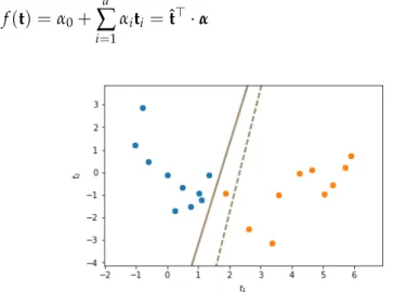
We have seen intask 1.2how a linear model can be used to obtain a separating hyperplane for classification. A drawback of this approach is the fact that the least squares error does not capture what we expect from an optimal separation. This is illustrated infig. 2.1. In this example the plane created by maximizing the distance to the nearest points of each class provides a better classification. One could equivalently look for the plane with the largest possiblemargin(in orthogonal direction) around it such that no data point is within the margin.
In this chapter we will see how this plane can be found and we will also treat the case of nonlinear separability. The resulting algorithm is known as Support Vector Machine (SVM) and it is one of the most famous algorithms in Machine Learning [4,5].
optimal separating hyperplanes
Let Ω = Rd, Γ = {−1, 1}. Instead of performing a least squares fit gfor given dataD := {(xi,yi)∈Ω×Γ|i=1, . . . ,n}and then using the hyperplaneg(t) =0as a separator, we now determine theoptimal margin hyperplane
f(t) =α0+
∑d i=1
αiti =ˆt>·α (2.1)
Figure 2.1: Optimal fit of a hyperplane to input data labelled with two classes.
The optimization is w.r.t. least-squares (dashed) and maximum minimum distance to nearest point (solid).
14 support vector machines
between two classes of points which can be separated linearly. To this end, we solve the constrained optimization problem
max
α∈Rd+1,∑di=1α2i=1
M subject toyi
ˆ xi>·α
≥ Mfor alli=1, . . . ,n.
This problem can be recast into its so-calledWolfe dual form max
β∈Rn
∑n i=1
βi− 1 2
∑n i,j=1
βiβjyiyjhxi,xjiΩ
subject to0≤βi ∀i=1, . . . ,n (OMH) and
∑n i=1
βiyi =0.
Now, f is given by f(t) =
∑n i=1
βiyiht,xiiΩ+b. (2.2)
Note that we can easily switch between the representations (2.1) and (2.2) by settingα0= band
(α1. . .αd)T =
∑n i=1
βiyixi.
Details can be found in [2, 4]. We still have to propose a suitable optimization algorithm to solve (OMH) and to determine the so-called biasb.
support vector machines
By slightly altering the optimization problem above, we obtain a so- calledsupport vector machine. To this end we add additional constraints to (OMH):
max
β∈Rn
∑n i=1
βi− 1 2
∑n i,j=1
βiβjyiyjhxi,xjiΩ
subject to0≤βi ≤C ∀i=1, . . . ,n (SVM) and
∑n i=1
βiyi =0.
for some constant C > 0. This can be interpreted as a so-called reg- ularization. It allows us to obtain a model which possibly represents a better generalization for unseen test data than in the unregularized case C = ∞. More specifically, the choice ofCwill introduce a trade- off between the minimization of the misclassification error and the maximization of the marginMfrom above.
The so-called support vectors are the xk for which βk > 0,k ∈ {1, . . . ,n}. The name hints at the fact that these are the necessary input data points, which span the vector (α1. . .αd)T that determines the hyperplane. To solve (SVM) we will use thesequential minimal opti- mization (SMO)algorithm. Note that for the linear SVM we considered so far, other solvers are more suitable. But the SMO algorithm can be easily adapted to the nonlinear SVM, which is introduced next.
Sequential minimal optimization
Algorithm 1OneStep algorithm to update the coefficients βi,βj and the biasbof f(·) =∑nl=1βlylh·,xliΩ+b
Input:Indicesi,j∈ {1, . . . ,n}. βoldj ← βj,βoldi ←βi
δ←yi (f(xj)−yj)−(f(xi)−yi) s←yi·yj
χ← hxi,xiiΩ+hxj,xjiΩ−2· hxi,xjiΩ γ←sβi+βj
ifs=1then
L←max(0,γ−C) H←min(γ,C) else
L←max(0,−γ) H←min(C,C−γ) end if
ifχ>0then βi ←min
max
βi+ δ
χ,L ,H else ifδ >0then
βi ←L else
βi ←H end if βj ←γ−sβi
Update function evaluations f(xl),l=1, . . . ,n b←b−12(f(xi)−yi+ f(xj)−yj)
The SMO algorithm [3] works in an iterative manner. At first the values forβandbare initialized (e.g. as0). In every iteration step we select two indicesi,j∈ {1, . . . ,n}and solve the quadratic optimization problem (SVM) by fixing allβk for indicesk ∈ {1, . . . ,n} \ {i,j}. Note, that this can be done exactly. To this end, one iterative step for the selected indicesi,jcan be found inalgorithm 1.
Task 2.1. Implement the function OneStep fromalgorithm 1, which takes one iterative step of the SMO algorithm for two selected indicesiandj.
16 support vector machines
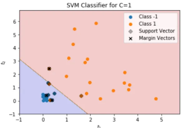
Figure 2.2: Support Vector Classifier forC=1.
Task 2.2. To have a small data set on which we can test our algorithm, we draw 20 two-dimensional vectors according to an exponential distribution withλ= 4in each of the coordinate directions, i.e. thej-th coordinate of the i-th vector is drawn i.i.d. according to [xi]j ∼ exp(4)for alli = 1, . . . , 20 and j = 1, 2. We assign the label −1 to these xi. Then, we draw 20 two- dimensional vectors according toexp(0.5) in the same way and assign the label1to them.
Task 2.3. Implement a functionSMOwhich initializesβ=0andb= 0and - in each iteration step - randomly picksi,j∈ {1, . . . ,n}such thati6= jand callsOneStepwith indicesi,jto perform an optimization.
(a) After the last iteration step, we need to compute a final estimate forb. To this end, calculate the median med of f(xk)−yk for all support vector indices k, i.e. allk ∈ {1, . . . ,n}for which βk > 0. Then, set b←b−med.
(b) Run the SMO function with10, 000iteration steps to compute a support vector classifier f for then = 40data points fromtask 2.2. Compute the results for C = 0.01, C = 1 andC = 100. For each C, plot the scattered data and the hyperplane corresponding to f = 0. Compare your results to the separating hyperplane computed by a linear least squares algorithm.
(c) Count the number of support vectors. Mark the correspondingxk in your scattered data plot.
(d) Furthermore, also count the number ofmargin defining vectors, i.e. the number of indicesk∈ {1, . . . ,n}for whichC> βk >0and mark the correspondingxk in the scattered data plot. An example for such a plot can be found infig. 2.2.
What influence does the parameterChave on the number of the support vectors and on the position of the separating hyperplane?
Now let us check how our classifiers perform if we evaluate them on some test data.
Task 2.4. Draw 2, 000test data points according to the distributions from task 2.2(1, 000points for class−1and1, 000points for class1). Evaluate the accuracy (percentage of correctly classified data points) for the LLS and SVM models calculated in tasktask 2.3.
The random picks ofi,jin the SMO algorithm can be very ineffective for large data sets. Therefore, we have to come up with a better heuristic to choose appropriate indices in each step of the SMO algorithm. There exist many heuristics to choose suitable indices in each step. We refer the interested reader to [3,4]. We will employ theKarush-Kuhn-Tucker conditions of the dual minimization problem:
KKTi := (C−βi)max(0, 1−yif(xi)) +βimax(0,yif(xi)−1). (2.3) Task 2.5. Repeattask 2.3 and task 2.4but instead of drawing the indices i,j for each SMO-step randomly, write an outer loop which iterates over all i ∈ {1, . . . ,n} and check if KKTi > 0. If this is the case, randomly pick a j 6= i for which 0 < βj < C. If no such j exists, randomly pick a j ∈ {1, . . . ,n} \ {i}. Subsequently, run theOneStep function for the pair (i,j). IfKKTi = 0 for eachior if the maximum number of OneStepcalls (10, 000) is reached, the algorithm terminates. Compare the results achieved with this heuristic with the results achieved by randomly pickingiandj. How do their runtimes compare?
nonlinearity –feature maps and kernels
A major drawback of the linear least squares approach and the support vector machines above is the fact that the resulting functions are linear.
However, in cases where the distribution of the input data is such that a linear hyperplane is not a suitable to classify the data, it is advantageous to consider nonlinear approaches. We already learned about a very simple nonlinear algorithm: k-nearest neighbors. Here, the separation is done by a nonlinear function. Next, we will learn about the nonlinear SVM.
Nonlinear SVM
The main reason for the huge success of SVMs in machine learning is due to the fact that we can slightly alter (SVM) and (2.2) to obtain nonlinear classifiers. To this end, we consider the so-calledkernel trick:
We change the scalar products to an evaluation of a kernel function K:Ω×Ω→R
ht,xiΩ −→K(t,x). (Kernel trick) In machine learning this is usually done by using a nonlinear feature map φ : Ω ⊂ Rd → V into a Hilbert space V (usually with higher dimension thand) and defining
K(t,x):=hφ(t),φ(x)iV.
18 support vector machines
In this way, we transform our input data by the feature map and can apply our SVM algorithm on the image ofφby using the scalar product inV. Let us have a look at a simple example.
Task 2.6. Generate50 uniformly distributed i.i.d. points which lie in{t ∈ R2 | ktk2 < 1}(e.g. by drawing uniformly distributed points in(−1, 1)2 until50of them are within the unit sphere) and label them by−1. Now generate 50data points, which are uniformly distributed in{t∈R2|1< ktk2<2} and label them by1.
(a) Fit a linear SVM forC= 10to the data and plot the scattered data as well as the separating hyperplane.
(b) Transform the data by the feature mapφ:R2 →R3defined by φ(t):= t1,t2,t21+t22
.
Fit an SVM forC=10to the transformed data. Plot the scattered data and the nonlinear separation curve in a2dplot (i.e. in the same way as in (a)). What does the feature map do and why does it work so well?
One of the most important theorems for kernel learning algorithms such as the nonlinear SVM isMercer’s theorem: It tells us that for each continuous, symmetric and non-negative definite kernel function K there exists a corresponding feature mapφ. However, for many famous kernels such as the Gaussian
Kσ(t,x):=exp −kt−xk2
Rd
2σ2
!
the corresponding vector spaceV can be infinite-dimensional and an explicit construction ofφcan be infeasible to compute. In these cases it makes much more sense to work directly with the kernelK.
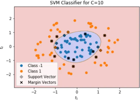
Task 2.7. Change your SMO code and your function evaluation of f from (2.2)such that it allows to use a kernel function instead of the scalar product of the input data, i.e. substitute all scalar products by the evaluation of the kernel function. Perform a SVM classification (C=10) with Gaussian kernel (σ = 1) for the data fromtask 2.6. Plot the scattered data and the nonlinear separation curve in a2dplot. The result should look similar tofig. 2.3.
k-fold crossvalidation
In practical applications the choices of the regularization parameterC as well as optional kernel parameters, such asσfor the Gaussian kernel, play an important role. The most common technique to determine these so-called hyperparametersiscrossvalidation. Here, the training data set is randomly split into k parts/foldsof approximately equal size. One fold is taken as test (or evaluation) data while the remaining k−1
Figure 2.3: Support Vector Classifier with Gaussian kernel forC=10,σ=1.
folds serve as input data for our algorithm. Subsequently, we take a different fold as evaluation data and the rest as input data and repeat the process k times until each fold has been used as evaluation data once. The (arithmetic) average of the k accuracies calculated on the evaluation data serves as our quality measure. This process is called k-fold crossvalidation.
Now, to determine the best choice of hyperparameters, we choose small candidate sets, e.g.C∈ {0.01, 0.1, 1, 10, 100},σ∈ {1, 10, 100}and run ak-fold crossvalidation for all possible combinations of parameter pairs. The pair(C,σ)with the best average accuracies in the crossval- idation process is the winner. The corresponding pseudocode can be found inalgorithm 2. Subsequently, the winning parameter set is usu- ally taken to learn an SVM on the whole training data, i.e. all kfolds.
The resulting model is then evaluated on the true test data, which has not been touched during the crossvalidation process. More details on this approach are given in [2,4] for example.
Algorithm 2Abstractk-fold crossvalidation scheme
Input: k ∈ N, training data D, possible combinations of hyperpa- rametersP.
Randomly splitDintokpartsD1, . . . ,Dkof (almost) equal size.
for allp∈ Pdo
for alli=1, . . . ,kdo
Run learner with input data∪j6=iDjand parametersp.
Evaluate resulting model onDi and store accuracyAi. end for
Average over the accuracies:Ap← 1k ∑ik=1Ai. end for
Determinepbest ←arg maxp∈PAp.
20 support vector machines
Figure 2.4: Four example images (28×28 pixels) from the MNIST data set (http://yann.lecun.com/exdb/mnist/).
application to real world data
We will now apply a support vector machine to a real-world classifica- tion problem.
Multi-class Learning
Up to now, we always considered classification problems, where our label set Γ was of size two, i.e. we just had two different classes. In real-world applications one often encounters so-calledmulti-classclas- sification problems, where |Γ| > 2. In this case, a very common idea is to use |Γ|(|Γ2|−1) pairwise classifiers, i.e. classifiers to discern between each possible pair γ1 6= γ2 of classes inΓ. To decide, in which class a data point t lies, each pairwise classifier is evaluated and the class γ∈Γto whichtis assigned the most wins.
In this way, we can apply standard two-class algorithms to solve multi-class problems. We refer to [2, 4] for more details on different approaches to multi-class problems.
The MNIST data set
TheMNISTdata set (http://yann.lecun.com/exdb/mnist/) consists of70, 000grey-scale images (28×28pixels) of handwritten digits. Four exemplary images can be found infig. 2.4. Our goal will be to construct an algorithm which is able to identify the correct digit from an image of the handwritten one.
You can either download and extract it by hand or use the following lines of code. As you see, you might need to install theurlliblibrary.
To this end, just runpip install urllib3in your shell.
# Load MNIST Data import os
import gzip
from urllib . request import urlretrieve
def download ( filename , source =’ http :// yann . lecun . com / exdb / mnist / ’):
print(" Downloading %s" % filename )
urlretrieve ( source + filename , filename )
def load_mnist_images ( filename ):
if not os . path . exists ( filename ):
download ( filename )
with gzip .open( filename , ’rb ’) as f:
data = np . frombuffer (f. read () , np . uint8 , offset
=16)
data = data . reshape ( -1 , 28 , 28) return data / np . float32 (256) def load_mnist_labels ( filename ):
if not os . path . exists ( filename ):
download ( filename )
with gzip .open( filename , ’rb ’) as f:
data = np . frombuffer (f. read () , np . uint8 , offset
=8) return data
X_train = load_mnist_images (’train - images - idx3 - ubyte . gz
’)
y_train = load_mnist_labels (’train - labels - idx1 - ubyte . gz
’)
X_test = load_mnist_images (’t10k - images - idx3 - ubyte . gz ’) y_test = load_mnist_labels (’t10k - labels - idx1 - ubyte . gz ’)
Scikit-Learn – A neat machine learning library in python
For the sake of understanding the basic programming and machine learning paradigms, we did (and will) implement the learning al- gorithms on our own. However, we will also learn how to use im- portant python machine learning libraries such as scikit-learn (http:
//scikit-learn.org). This is an efficient and easy-to-use library in which we can find variants of all algorithms we have learned about so far (LLS,k-NN, SVM) and many more.
Task 2.8. Make yourself familiar with theSVCfunction inscikit-learn, which implements a support vector classifier.
(a) Choose a random subset of size500from the MNIST training data and use this as your new training data set for crossvalidation. Perform a 5-fold crossvalidation SVM to determine the optimal parameters among C ∈ {1, 10, 100}andγ = 2σ12 ∈ {0.1, 0.01, 0.001}. (Hint: You can use thescikit-learnfunctionGridSearchCV.)
(b) Use the determined optimal parameters to learn a support vector clas- sifier on a random2, 000point subset of the MNIST training data and evaluate the confusion matrix and the accuracy on the whole MNIST test data set. (Hint: You can use thescikit-learnmodulemetrics.) Is our approach of picking a different training set in step (b) – and learning with the optimal parameters from (a) – valid? Are there potential pitfalls?
22 support vector machines what we did not cover...
non-numerical data Note that the feature map approach allows us to also classify data which does not reside in an Euclidean space by building appropriate feature maps that assign a value inVto each element of the input data. This is often very useful when it comes to practical applications where data is not directly given as numerical values or vectors.
kernel choice The kernel can also be chosen by crossvalidation over a finite set of fixed kernel functions for instance. However, if we have some a priori problem knowledge (such as smoothness of the
“true” separation function), we can exploit this in order to choose an appropriate kernel, see also [1].
regression The linear least squares and the k-nearest neighbors algorithms also apply to the regression case, where we look for a func- tion f such that f(xi)≈ yi and theyi can take arbitrary values inR– instead of only discrete ones as in classification. However, for support vector machines this is not so straightforward since our optimization problem (SVM) originated from the optimal margin hyperplane for- mulation. Nevertheless, there also exists a support vector machines regression algorithm based on the minimization of the so-called ε- insensitive loss function, see [4].
references
[1] F. Cucker and D. Zhou.Learning theory. Cambridge Monographs on Applied and Computational Mathematics, 2007.
[2] Trevor Hastie, Robert Tibshirani, and Jerome Friedman. The El- ements of Statistical Learning. Springer Series in Statistics. New York, NY, USA: Springer New York Inc., 2009. url: https : / / web.stanford.edu/~hastie/ElemStatLearn/download.html. [3] John Platt. Sequential Minimal Optimization: A Fast Algorithm for
Training Support Vector Machines. Tech. rep. 1998.
[4] B. Schölkopf and A. Smola.Learning with Kernels – Support Vector Machines, Regularization, Optimization, and Beyond. The MIT Press – Cambridge, Massachusetts, 2002.
[5] V. Vapnik.Statistical Learning Theory. John Wiley & Sons, 1998.