The Bitvector Machine: A Fast and Robust Machine Learning Algorithm for Non-Linear Problems

(1)

The Bitvector Machine: A Fast and Robust Machine Learning Algorithm for Non-Linear

Problems

Stefan Edelkamp and Martin Stommel

Research Group Artificial Intelligence, Universit¨at Bremen Am Fallturm 1, 28359 Bremen, Germany

{edelkamp,mstommel}@tzi.de

Abstract. In this paper we present and evaluate a simple but effec- tive machine learning algorithm that we callBitvector Machine: Feature vectors are partitioned along component-wise quantiles and converted into bitvectors that are learned. It is shown that the method is efficient in both training and classification. The effectiveness of the method is analysed theoretically for best and worst-case scenarios. Experiments on high-dimensional synthetic and real world data show a huge speed boost compared to Support Vector Machines with RBF kernel. By tabulating kernel functions, computing medians in linear-time, and exploiting mod- ern processor technology for advanced bitvector operations, we achieve a speed-up of 32 for classification and 48 for kernel evaluation compared to the popular LIBSVM. Although the method does not generally outper- form a SVM with RBF kernel it achieves a high classification accuracy and has qualitative advantages over the linear classifier.

Keywords: classification, support vector machine, time/accuracy trade- off

1 Introduction

Due to the flexibility of kernel functions, statistical machine learning with Sup- port Vector Machines, SVMs for short [1], is one of the most successful approaches for classification applications [2].

The number of support vectors learned affects training and classification speed. Bordes et al. ([3]) assume that not all training samples are equally relevant for the resulting model. Their LASVM¹ implementation achieves a significant speedup during training by using an online approach, where the margin is determined from a small subset of the input data. Important modeling decisions can be reached even without taking into account the class label of a data point.

The measurement of the model accuracy also affects the training speed.

Joachims’ [4] SVMLIGHT² implementation achieves a significant speed-up in

1 http://leon.bottou.org/projects/lasvm

2 http://svmlight.joachims.org/

(2)

the estimation of the leave-one-out error by evaluating the Lagrange multipliers and slack variables of a trained model. This saves the retraining of the model for every sample left out. Tsang et al. [5] propose a radical simplification of the model by approximating the convex hull of the training data by an enclosing ball in the high-dimensional feature space. The allowed error of the approximation is a parameter of the algorithm. The method works iteratively to find the centre of the ball. The idea of using a reduced set of support and also non-support vectors to define the decision border has also been used in previous approaches [6, 7]. Influences stem for example from approximate k-nearest neighbours [8] or computational geometry [7].

There are also fast SVM implementations with linear kernels that exceed the library used in this paper (LIBSVM³) by far, e.g. LIBLINEAR⁴ and Leon Bottou’s stochastic gradient descent SVM⁵. However, for complex data where single classes comprise multiple distant sub-clusters, non-linear kernels achieve a higher accuracy. Chang et al. [9] achieve a speed-up of a second order polynomial classifier by using optimisation techniques usually reserved for linear kernels.

Zhang et al. [10] compute a low rank linear approximation of the kernel matrix of a non-linear kernel and evaluate it by a linear SVM.

The dimensionality of the input data affects the speed of the classification as well, but it also often causes a numerical instability known as the curse of dimensionality. It is described [11] as a general unreliability of distance computations for data sets where minimum and maximum distances approximate with rising dimensionality. The effect can be reduced by choosing a smaller norm than the Euclidian [12], but taking high roots is numerically difficult, too.

In the application of machine learning algorithms to image and video data, a binary discretisation of the popular SIFT (Scale Invariant Feature Transforma- tion [13]) feature vector does not suffer from this effect [14], whereas the original SIFT representation does. Although a feature binarisation is a dramatic simplification of the input data, it has been observed for SIFT and SURF (Speeded Up Robust Features [15]) descriptors that the matching accuracy does not decrease significantly [16]. In some cases the relative error rates even decreased.

Moreover, the length of the descriptors is reduced by a factor of 8 for SIFT (128 dimensions, usually implemented as single bytes) and by a factor of 32 for SURF (64 dimensions, usually implementated by 4 byte floating point values). These advantages are highly relevant for robotics applications as SURF or SIFT are called at a high frequency in Simultaneous Localisation and Mapping (SLAM)⁶. In this paper, we study the findings on feature binarisation in a more general setting. A brief summary of SVMs allows us to introduce the method under the

3 http://www.csie.ntu.edu.tw/∼cjlin/libsvm

4 http://www.csie.ntu.edu.tw/∼cjlin/liblinear

5 http://leon.bottou.org/projects/sgd (this algorithm has been ported by us to the GPU for an even faster evaluation time)

6 http://openslam.org

(3)

notion of aBitvector Machine⁷. We discuss conditions under which the binarisation of a feature vector is appropriate. We observe that the Hamming distances between binarised input vectors are discrete and limited. This allows a number of important code optimisations for kernel evaluation, most notably the use of look-up tables and native processor instructions. In contrast to previous work [16]

where no dedicated CPU instructions are used, we can therefore quantify the main advantage of the method: the speed in the kernel evaluation. For transform- ing the input data from floating point to binary strings we exploit that medians can be computed efficiently. By replacing the medians byq-quantiles, we generalise the Bitvector Machine to a Multi-Bitvector Machine. The method allows for a wider range of possible time-accuracy trade-offs and avoids some worst-case behaviours of the single-bit binarisation. In the empirical part of the paper we evaluate the (single-bit) approach in three different experimental settings. The first and second ones comprise artificial data (a Mixed Gaussian Distribution).

The third one deals with real-world data from a face recognition application. As a result we achieve a several fold speed-up in the classification with only a small loss in accuracy compared to LIBSVM. As far as pure kernel computations are concerned, the method also accelerates training, although this is not deepened in the paper.

2 Support Vector Machines

Raw data presented to a supervised statistical machine learning algorithm [17]

can be arbitrarily complex and is often mapped to a set of numerical values, called the feature vector. The classification problem deals with the prediction of the labellof previously unknown feature vectorsx∈R^dthat constitute the test data. During training, a partitioning of the feature space R^d is learned, where each partition is assigned a labell from a small setLbased on a set of training samples (x1, l1), . . . ,(xk, lk) ∈ R^d×L with known labels. The challenge is to approximate the unknown distribution without overfitting the training data.

Support Vector Machines [1], SVMs for short, achieve this task by learning coefficients for a kernel mapping to a high-dimensional space, where a linear class border is spanned up by a number of support vectors that outline the data. We keep the presentation brief as there are text books on SVMs and related kernel methods [2, 18]. Theoretically, it should be sufficient to determine the class border by just three support vectors. However, it is not known in advance if any of the known kernels realises a suitable mapping. The use of generic kernels instead leads to a much larger number of support vectors (which critically influence classification time). In the worst case finding a separating hyperplane takes quadratic time in the number of data points.

7 The term machine links to the fact that the classifier realises a mathematical function, sometimes referred to as a machine.

(4)

The classification rule for a two-class non-linear classification functionφis

f(x) = sign

s

X

i=1

βi(φ(xi)·φ(x)) +b

!

, (1)

wherexiis theith ofs≤ksupport vectors,βi is a coefficient that includes class label and Lagrange multiplier from the optimisation, and b is some additional translation constant. Assuming a kernel functionK(u,v) =φ(u)·φ(v) we get

f(x) = sign

s

X

i=1

βi·K(xi,x) +b

!

, (2)

which does not refer directly toφ, known as the kernel trick.

SVM training is a convex optimisation problem which scales with the training set size rather than the feature space dimension. While this is usually considered to be a desired quality, in large scale problems it may cause training to be impractical and classification to be time consuming.

The corpus of SVM applications is large and encompasses many areas of computer science [2]. As kernel functions can be complex, the application of SVMs is large and kernels can be designed to cover simple regression to neural network approaches [19] and time series [20]. However, linear kernelsK(u,v) = u·v+g or Gaussian (RBF) kernels K(u,v) = exp(−γku−vk²), γ ∈ R are the ones that are most commonly used. In the second case, a SVM is a function that itself defines a Mixed Gaussian Distribution [21] and is related to Radial Basis Networks and Neuronal Nets with one hidden layer. Since the optimisation objective is high accuracy instead of a low number of support vectors, a Mixed Gaussian input will be usually modeled by multiple centres per Gaussian in the SVM.

The running time for classifying one vector is O(sde), where e is the time to evaluate the exponential. Practical SVM implementations might assume the input data to be normalised to avoid numerical difficulties.

3 Bitvector Machine

A Bitvector Machine, BVM for short, is an SVM with a binarisation (Boolean discretisation) of the input: All vectorsxi∈R^d, 1≤i≤k, used in the training phase and all vectors evaluated in the test phase are mapped to {0,1}^d. The labels remain unchanged. The results are then fed into a SVM.

The median of k totally ordered elements is the element in the bk/2c-th position after sorting. Median selection can be performed in linear time [22]. Let

¯

x= (¯x¹,¯x², . . . ,x¯^d)^> ∈R^d be the component-wise median of the input vector, i.e. ¯x^j is the median of thej-th vector components ofx₁, . . . ,x_k.

The BVM maps (training and test) vectors x ∈ R^d to binary strings z = (z¹, z², . . . , z^d)^> ∈ {0,1}^d as follows: For each j, 1≤j ≤d, we have z^j = 0 if and only ifx^j <x¯^j. Otherwisez^j is set to 1.

(5)

Theorem 1 (Time Complexity Single-Bit Binarisation). The binarisation of allx_i∈R^d,1≤i≤k, takes timeΘ(kd).

Proof. Computing all component-wise medians of vectors xi ∈ R^d, 1 ≤ i≤k, i.e. ¯x, requires O(kd) time. Thresholding all vectors xi ∈ R^d component-wise with ¯xcan be executed in time O(kd). Considering the input size of the data, the timeO(kd) is optimal.

By using q quantiles instead of the medians (where q = 2) we can create more detailed feature representations of longer word length. Quantiles represent a subdivision of the domain of a random variable intoq consecutive partitions of equal cumulative density 1/q. The respective thresholds can be read from the cumulative distribution function or by recursively computing medians (if qis a power of 2). The assignment of a random value to itsη-th, 1≤η ≤q, quantile can be done in log-time by arranging the thresholds in a balanced binary tree.

The representation of the index η of a quantile requiresm=dlgqebits.

AMulti-Bitvector Machine, MBVM for short, maps (training and test) vectors x∈R^d to binary stringsz= (z¹, z², . . . , z^md)^> ∈ {0,1}^md, m=dlgqe. In order to binarise ad-dimensional feature vector, we compute quantiles of fixedq independently for every dimension. The binary feature vector is the concatena- tion of alldquantile indicesη, the resulting length is thus mdbits. Computing all component-wise quantiles of vectors x_i ∈ R^d, 1 ≤ i ≤k, requires O(mkd) time, as computing the list of all quantiles of akelement set takes timeO(mk) (see Ex. 9.3-6, p. 223 in [23]). As q < k and, subsequently, m < dlgke this approach is still faster than sorting with its time complexity ofΩ(klgk).

Corollary 1 (Time Complexity Multi-Bit Binarisation). The multi-bit binarisation of all xi ∈ R^d, 1 ≤i ≤ k, using q-quantiles takes time O(mkd), with m=dlgqe.

Instead of reducing the dimension as done in related work, e.g. on random projections [24], we enlarge it. The motivation is that the increase in dimensionality is compensated by the speed-up by the lower bit-rate.

The computation of median (quantile) based binary representation corresponds to a partitioning and re-labeling of the feature space. If we were to split the data iteratively, we would build a kd-tree in O(nlgn) time [25], for which rectangular range queries takeO(√

n+k) and membership queries takeO(lgn) time [26]. In contrast, in the BVM the median splits are chosen independently of each other, one in each vector component. The binarisation therefore defines a partitioning of the feature space into regions, where all separating hyperplanes intersect in one point. Geometrically, it can be interpreted as moving the origin of the Cartesian coordinate system to ¯xand representing each resulting orthant by a bitvector{0,1}^dthat indicates the position relative to the iso-oriented hyperplanes. The bitvectors correspond to nodes in addimensional hypercube (an edge in the hypercube has Hamming Distance 1).

(6)

Letψ be the mapping that performs the binarisation. We have

f(x) = sign

t

X

i=1

δi·K(ψ(xi), ψ(x)) +g

!

. (3)

Due to a different training, the number of support vectors t, weights δ and biasgmight be different from the original values (s, β, bin Eq. 2). Moreover, as K(ψ(u), ψ(v)) =φ(ψ(u))·φ(ψ(v)), we see that we are actually dealing with a different kernel that transforms data via φ◦ψ from R^d first into the Boolean space{0,1}^d before lifting it into higher dimensions.

Because of the symmetry property, distance metrics based on an element by element comparison (like Euclidean or Hamming distance) in {0,1}^d yield onlyd+ 1 different values. All possible results of the kernelK(ψ(xi), ψ(x)) can therefore be precomputed.

For the Gaussian kernelK(ψ(u), ψ(v)) = exp(−γkψ(u)−ψ(v)k²) the term kψ(u)−ψ(v)k²can only yieldd+1 different values. For the Euclidean norm they range from 0 todand equal the Hamming distance of the kernel arguments. By applying the parameterγ and the exponential to these values, the whole kernel can be precomputed and stored in a table. This avoids the repeated time consuming computation of the exponential during classification. The Hamming distance can be computed by applying the population count instruction (counting the number of bits set) to the bitwise XOR disjunction of the arguments.

Precomputing kernels reduces training and classification time. Because training is done only once, we focus on the latter.

Theorem 2 (Time Complexity Single-Bit Classification).Assumingdto beO(w)for the computer word widthwand native population count, the running time for classifying one bitvector is O(t+d), where t is the number of support vectors.

If population count is not native on the word level, then the classification of one vector has the complexityO(d+tlg^∗d), wherelg^∗dis the iterated logarithm, i.e. the height of the shortest tower of powers 2²^... that equals or exceedsd.

Proof. Computing the binarisation ψ(x) of the test vector x takes time O(d).

The population count and XOR to be executed on the word level to compute the Hamming Distance run in O(1). Given that the kernel is tabulated, we require only lookups to the kernel table, so that multiplication with a constant and addition have to be executed t times to evaluate the classification formula Pt

i=1δi·K(ψ(xi), ψ(x)).

For larger values ofdpopulation count can be done inO(lg^∗d) by iterating the HAKMEM algorithm⁸.

The second part of the theorem assumes large word widthwand is mainly of theoretical interest.

8 David Eppstein, http://11011110.livejournal.com/38861.html

(7)

Assuming that the binary representation of the bitvectors due to computing the quantiles still fits into a computer word widthw, for an MBVM computing the binarisation of the test vectorxtakes timeO(md). Hence, the running time for classification generalizes to O(t+md) with m being the dual logarithm of the number of quantiles considered.

Corollary 2 (Time Complexity Multi-Bit Classification).Assumingdto beO(w)for the computer word widthwand native population count, the running time for classifying one bitvector isO(t+md), where tis the number of support vectors.

If population count is not native on the word level, then the classification of one vector has the complexityO(md+tlg^∗(md)).

The entropy for one split along the median is certainly maximal as long as class labels are not taken into account. But even for simplified Mixed Gaussian Distributions (2D, shifted mean, same deviation but same amplitude) entropies can only be approximated [27].

The number of regions distinguishable by the BVM rises exponentially with dimensionality. For dimensionality d we have 2^d possible regions. As we split the data component-wise, the BVM corresponds to a static decision tree that has depth d and that is independent of the number of elements. An explicit construction of such a tree, however, is not required. In contrast to SVMs, the binarisation automatically normalises the input data to the unit hypercube.

Because the BVM is trained the same way as a SVM, we can still use cross- validation or leave-one-out-validation to estimate the classification error.

4 Case Studies

One question is if and when the binary kernel is better than a linear one. If we assign each vector{0,1}ⁿwith even population count with class 1 and each vector{0,1}ⁿ with odd population count with class 2, then we generalise the XOR problem to higher dimension (the minimal Hamming distance of two elements class in one class is two). This is clearly not linearly separable, but the BVM can find a perfect classification.

This clearly is a best-case scenario, but we can argue that linearly non- separable but binary separable examples are common in practice. One reason for this is that many classes underly the principles of differentiation and com- position. Let us assume for example a set of images of noses, either taken from a left angle or from a frontal perspective. Although left noses are visually and numerically similar to each other, they differ strongly from frontal noses and occupy a separate region in feature space. The combined class nose, however, is activated by features from both differentiations. The dispersed placement of multiple clusters of sub-classes in feature space can easily create non-linearly separable situations, especially in multi-class problems. Moreover, real-world data often comes from independent or principle component analyses. As a result, feature distributions for different sub-classes tend to be aligned with the coordinate axes.

(8)

One worst-case scenario for the BVM in two dimensions is a checker-board layout of two classes because after two orthogonal cuts all fields of the checker- board that fall into the same quadrant are represented by the same bitvector and with it the same class. For this theoretical setting, the SVM calls for several support vectors and likely an overfitting of the data. If the number of Gaussian kernels is small and the dimension is high, the BVM has good chances to find a discriminative partitioning. As a result, feature binarisation preserves high selectivity and lifts the curse of dimensionality.

However, if we were to use a MBVM with as many quantiles as the checker- board size, the worst-case behavior would be avoided and we would encounter a best-case scenario with accurate class boundaries.

Even though entire orthants collapse to single data points on the hypercube, the Gaussian weighting of the binary vectors still preserves at least some geo- metrical meaning. The weights for a specific class are propagated nonlinearly from one orthant to another via shared hyperedges. For shared hyperedges the Hamming distance of the associated bitvectors is one.

5 Experiments

We performed the experiments on one core of a desktop computer (model Intel Core i7 920 CPU 2.67 GHz) running Ubuntu 10.10 (Linux kernel 2.6.32-23- generic) with 24 GB main memory. With such memory capacity, there was no need to use virtual memory. We compiled all programs using GNU C++compiler (gccversion 4.3 with option -O3and-mpopcnt).

For the implementation of the BVM we have extended LIBSVM to support bitvector manipulation based on a precomputed kernel and native population counting. LIBSVM is chosen because it is well known, widely used, and easily extendible. It uses a one-versus-one strategy for multi-class problems.

The use of SVM implementations aiming at higher training speed [3, 4] would not provide a deeper insight because our method aims at testing speed. The BVM is also not in contradiction to approximative methods working on reduced sets [5–

8]. It would therefore be possible to combine a fast binary vector representation with a small approximated set of support vectors in order to achieve an even higher speed-up. However, in favour of the clarity of the presentation we refrain from such combined approaches.

We evaluate the BVM in two synthetic and one natural scenarios.

5.1 Artificial Data

To validate our ideas experimentally, we produced training and test data for two and five-class problems in a random process with defined statistical properties.

For each class we realised a sampling of a Mixture of Gaussians. The mean µi, i= 1,2, . . . of each multivariate Gaussian

pi(x) = 1

(2π)^d²|Σ|¹²exp

−1

2(x−µi)^>Σ⁻¹(x−µi)

(4)

(9)

is placed in the unit hypercube. The bandwidth is set globally in the main diagonal of the covariance matrixΣfor all Gaussians. The number of Gaussians is set individually for every experiment.

The maximum likelihood estimate (Bayes) of the Mixed Gaussian distribution is used as the ground truth to which an SVM and the proposed method are compared. Linear kernels are used to detect linearly separable situations.

The difficulty of the created problems is controlled by adjusting the bandwidth of the Gaussians for a specific accuracy of the maximum likelihood estima- tor. If we keep the number of Gaussians fixed and increase the dimensionality, we have to increase the bandwidth, too. Otherwise the overlap between the Gaussians decreases and the difficulty of the problem changes. The bandwidth of the kernel is therefore a parameter of the experimental setting. It exhibits a strong influence on the resulting estimate. We therefore set it manually, although Silverman indicates a dependency of the bandwidth on the root of the dimensionality [28].

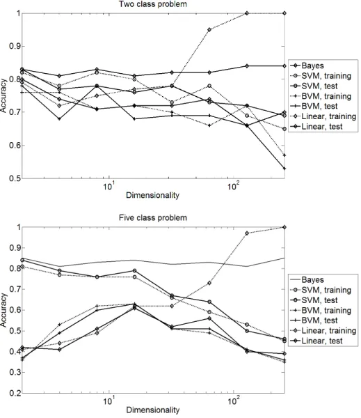
First Scenario As a parameter of the synthetic experiment, we choose the bandwidth to provide accuracy values to be in the range [0.8,0.85]. For determining the classification accuracy (on the training and test sets) we conducted two experiments, one for a two-class problem and one for a five-class problem both with rising dimension (dimensionalities 2, 4, 8, . . . , 256). The two-class problem is modeled by three Gaussians per class at uniformly distributed random posi- tions in the unit cube. With 5 Gaussians per class, the five-class problem is more complex. Each Gaussian is sampled 70 times. The data set is randomised and split into equally sized training and test sets. The parametersC (a weighting of the slack variables in the optimised function) and γ of both the BVM and the RBF kernel of LIBSVM are optimised in a grid search using the Python scripts provided by LIBSVM. For the Gaussian kernel and the BVM the training set is further subdivided in order to perform a five-fold cross validation for parameter selection.

The plots in Fig. 1 show that the BVM solves the problem surprisingly well, given the limitation that the BVM does not represent any gradual or continuous feature values.

For smaller dimensions and the two-class problem, all methods lead to very similar results with a small advantage for the SVM with Gaussian kernel. The results of the BVM are comparable to those of the linear classifier, with chang- ing winners. For the five-class problem, the results are clearer. Training and test results are closer for smaller dimensionalities and the BVM achieves results between the SVM with Gaussian and linear kernel, although closer to the linear one. The recognition rate of the BVM has a maximum at 32 dimensions. It seems that lower dimensions limit the capacity to represent information.

For more than 32 dimensions, the accuracy drops significantly for all methods.

The pronounced divergence between the training and test results of the linear classifier indicates heavy overfitting. The Gaussian kernel does not show this overfitting but the bad results indicate a clear failure, too. Although the cross-

(10)

Fig. 1.First scenario: Accuracy for the SVM (RBF and linear kernel) and the BVM

validation on subsamples of the training set leads to better estimates of the final recognition rate, it cannot compensate for missing information.

In summary the accuracy of all classifiers is limited, so our experiment may be overly complex. Even the linear kernel might be competitive if additional application constraints are taken into account. It must also be said that the difficult class borders in this Gaussian mixture do not have much in common with data sets from pattern recognition tasks: In such applications, the feature vector often represents the similarity of a query object to a set of prototypes, where each

(11)

Fig. 2.CPU time measured for the classification of the data sets in the first scenario.

The original real valued data is classified by an SVM with Gaussian kernel. The binary data refers to the BVM.

similarity is stored in one dimension. Consequently, the class border would not normally cross a coordinate axis multiple times. The effect is even reinforced by the common use of coordinate transforms such as principle component analysis.

In matters of CPU time we see a drastic decrease in computation time for the BVM. Figure 2 shows that we obtain a huge speed-up that additionally increases with the dimension of the problem. The maximum increase of performance was a factor of 32 for the two class problem in 128 dimensions. The increase in CPU time at d = 256 for the BVM can be explained by the increased word length.

Here all word level operations have to be executed four times on a 64 bit machine. For bigger dimensions, computer architecture and compiler must be taken stronger into account. We have not measured the time for the preprocessing step.

However, it seems obvious to us that a loop over ddimensions in the binarisation of a feature descriptor is uncomparably faster than the computation of dot products to thousands of d-dimensional support vectors in the classification of one descriptor.

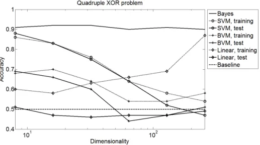
The Second Scenario represents the above-mentioned high-dimensional XOR problem but with noisy data. To this end, we centre the Gaussians of our Gaus- sian Mixture at the corners of the unit hypercube and assign class labels to the Gaussians as described above. The bandwidth is adjusted so that the Bayes classifier achieves an accuracy of 90%–92% using the known distribution.

Figure 3 shows the results of the proposed method and the SVM using the RBF and linear kernel. The Gaussian Mixture consists of four planar XOR problems placed at random sides of the unit hypercube of dimensionality 8, 16, . . . , 256). A planar XOR problem consists of four Gaussians at the corners of a square with diagonally different class labels. Each Gaussian is sampled 70 times.

The best results can be seen for the SVM using the RBF kernel. The output of

(12)

Fig. 3. Second scenario: Accuracy for a two class problem including four planar xor problems

the BVM follows the SVM at a lower level. The linear classifier fails completely because it cannot represent the non-linear class borders.

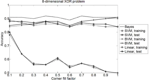
Figure 4 shows the results for an 8-dimensional XOR arrangement of varying sparseness. For this distribution, Gaussians are randomly placed in a certain percentage of all corners and sampled 100 times each. For a sparse filling of 10%, the distribution still seems linearly separable. However, with increasing density the linear classifier quickly approaches random, whereas the BVM im- proves gradually and finally outperforms the SVM with RBF kernel (corner fill factor≥0.5).

This good result shows that the interpretation of the BVM as a simplified approximation of the SVM depends on the understanding of the data (and study- ing the data is always a good start). If it is not known how the data corresponds to the described case scenarious, then the BVM must be considered as a non- parametric, simplified method and the results can be inferior to the SVM. If it is known that the data corresponds to a good case scenario, then we use the BVM as a model based method that benefits from our prior knowledge about the data.

5.2 Real World Data

The Third Scenario is a Computer Vision task, where SIFT descriptors [13] are classified into 16 classes (15 classes representing different parts of a face plus one background class). Additionally to the original SIFT method, we also tested a variation that takes into account that faces are shown in an upright orientation in most images. Without going into detail, we can say that the original SIFT

(13)

Fig. 4.Accuracy for a non-linear, 8-dimensional class arrangement of increasing complexity

method is rotationally invariant, i.e. different rotated versions of the image result in approximately the same feature vector. Our variation in contrast (marked as ’absolutely oriented’ in Tab. 1) is selective to orientation, so different rotated versions of the same visual pattern can be distinguished. In both cases the binarised feature vectors have 128 bits, so they can be compactly stored in two 64-bit words.

We evaluate the effectiveness of population counting on the machine and study the speed-ups obtained for sole kernel evaluations (Table 2) and whole vector classifications (Table 3). We compare the LIBSVM implementation with the BVM in two settings, one with a precomputed 16-bit population count lookup- table (2¹⁶entries), one with the native population count (__builtin_popcountll).

We run three examples for each setting to show that the variance in the running times is small. The table documents a speed-up factor of 48 in the 116 million kernel comparisons and an improvement by a factor of 17 for the entire classi-

Table 1.Accuracy [%] for SIFT data sets of different size and class distribution. There are 15 foreground classes and one background class. The samples are randomised and split into equally sized training and test sets.

Feature vector SIFT SIFT, absolutely oriented

Foreground samples per class 20 20 125 250

Background samples 2000 2000 1125 2250

Classifier Training Test Training Test Training Test Training Test

LibSVM, RBF 73.4 74.0 79.9 79.1 84.7 85.6 86.8 87.9

BVM, RBF 67.2 67.3 74.0 75.0 82.4 83.2 84.2 85.1

LibSVM, linear 99.1 60.7 97.7 70.5 94.6 77.4 90.9 79.6

(14)

Table 2. Evaluation time [s] for 116 072 232 kernel computations. The first column gives the result for LIBSVM using the Gaussian kernel. The second column gives the results for the BVM, where a look-up-table for 16-bit wide sub-words of the feature vector is used for the computation of the population count. In the last column, the native 64-bit population count CPU instruction is used.

No LIBSVM BVM, 16-bit-popcnt BVM, 64-bit popcnt

1 48.36 2.16 1.00

2 48.27 2.16 1.00

3 48.59 2.14 1.01

Table 3.Time [s] for classifying 16 788 vectors in 16 classes, 6914 support vectors.

Kernel computation using all support vectors No LIBSVM BVM, 16-bit popcnt BVM, 64-bit popcnt

1 39.44 4.01 2.84

2 39.45 4.01 2.81

3 39.71 4.00 2.71

only support vectors withβ6= 0

1 3.46 2.27

2 3.45 2.28

3 3.46 2.28

fication process. Further speed-ups might be achieved by using a one-versus-all strategy for multi-class problems instead of the one-versus-one strategy implemented in LIBSVM.

The difference in CPU time between the sole kernel computation and the whole classification indicates a strong influence of the code analysis and gener- ation of the compiler, since the number of kernel computations has been equal in both experiments, and the optimisation flags too.

Table 1 shows for different SIFT variations and different class distributions that despite the high speed-up the accuracy of the BVM is on average (from the cross validation) close to that of the SVM. The remaining gap seems statistically significant when comparing the results of the training and test sets. However, it becomes lower with increasing sample size. In comparison to the linear classifier, the BVM is clearly better. For the larger data sets, the BVM is closer to the Gaussian SVM than the linear one. The good results match findings in [16] where the classification accuracy (measured in error rates) has been shown to behave well for other Computer Vision Tasks, too.

6 Conclusion

We proposed a machine learning algorithm whose advantages result from a dramatic simplification of the input data. Discretisation certainly has limits in the accuracy of class distributions that are not iso-oriented. We argue, however, that iso-oriented classes with non-linearly separable sub-classes occur in many pattern recognition tasks.

(15)

The rising number of positive results in discretising feature vectors into bitvectors prior to the learning process shows that the effectiveness and efficiency of the binarisation in the BVM is an exciting phenomenon. Especially for a growing number of dimensions, where we lack a visual interpretation and where unexpected results like the curse of dimensionality have been measured, research might have concentrated on aspects that do not discriminate well. Even though binarisation reduces the information in the input considerably our experiments show that the results are often of acceptable quality, sometimes even better than the original unabstracted input.

Our experiments on synthetic and real data show that the accuracy of the BVM approximates (and in special cases exceeds) the accuracy of a SVM with RBF kernel better than a linear classifier, but is up to 48 times faster in the kernel computation and up to 32 times faster in classification. These results confirm our theoretical proof of the efficiency of classification and binarisation.

Compared to a linear classifier, the accuracy of the BVM is usually higher or equal. Furthermore, the BVM has the ability to model non-linearly separable problems where the linear classifier fails. Together with an improved empirical basis we provided insights that increase the understanding of when and why the approach works well, especially for large feature vectors. The BVM therefore allows for a welcome new trade-off between accuracy and running time for non- linear problems. The use of q-quantiles withq > 2 in the MBVM can improve the accuracy by the cost of time performance. Hence, the approach is expected to be applicable to problems that are not iso-oriented.

References

1. Vapnik, V.N., Chervonenkis, A.Y.: Theory of Pattern Recognition [in Russian].

Nauka, USSR (1974)

2. Cristianini, N., Shawe-Taylor, J.: An Introduction to Support Vector Machines and Other Kernel-based Learning Methods. Cambridge University Press (2000) 3. Bordes, A., Ertekin, S., Weston, J., Bottou, L.: Fast Kernel Classifiers with Online

and Active Learning. Journal of Machine Learning Research6(September 2005) 1579–1619

4. Joachims, T.: Learning to Classify Text using Support Vector Machines. Kluwer (2002)

5. Tsang, I., Kocsor, A., Kwok, J.T.: Simpler core vector machines with enclosing balls. In Ghahramani, Z., ed.: 24th International Conference on Machine Learning (ICML), New York, NY, USA, ACM (2007) 911–918

6. Burges, C.J.C.: Simplified Support Vector Decision Rules. In: In Proceedings of the Thirteenth International Conference on Machine Learning (ICML), Morgan Kaufmann (1996) 71–77

7. DeCoste, D.: Anytime Interval-Valued Outputs for Kernel Machines: Fast Sup- port Vector Machine Classification via Distance Geometry. In: Proceedings of the International Conference on Machine Learning (ICML). (2002) 99–106

8. Decoste, D., Mazzoni, D.: Fast query-optimized kernel machine classification via incremental approximate nearest support vectors. In: In International Conference on Machine Learning (ICML). (2003) 115–122

(16)

9. Chang, Y.W., Hsieh, C.J., Chang, K.W., Ringgaard, M., Lin, C.J.: Training and Testing Low-degree Polynomial Data Mappings via Linear SVM. Journal of Ma- chine Learning Research11(2010) 1471–1490

10. Zhang, K., Lan, L., Wang, Z., Moerchen, F.: Scaling up Kernel SVM on Limited Resources: A Low-rank Linearization Approach. In: International Conference on Artificial Intelligence and Statistics (AISTATS). (2012)

11. Beyer, K., Goldstein, J., Ramakrishnan, R., Shaft, U.: When Is ”Nearest Neighbor”

Meaningful? In: Int. Conf. on Database Theory. (1999) 217–235

12. Aggarwal, C.C., Hinneburg, A., Keim, D.A.: On the Surprising Behavior of Dis- tance Metrics in High Dimensional Space. In: Int. Conf. on Database Theory.

(2001) 420–434

13. Lowe, D.G.: Object Recognition from Local Scale-Invariant Features. In: Interna- tional Converence on Computer Vision (ICCV). (1999) 1150–1157

14. Stommel, M., Herzog, O.: Binarising SIFT-Descriptors to Reduce the Curse of Dimensionality in Histogram-Based Object Recognition. In Slezak, D., Pal, S.K., Kang, B.H., Gu, J., Kurada, H., Kim, T.H., eds.: Signal Processing, Image Pro- cessing and Pattern Recognition, Springer (2009) 320–327

15. Bay, H., Ess, A., Tuytelaars, T., Gool, L.J.V.: Speeded-Up Robust Features (SURF). Computer Vision and Image Understanding110(3) (2008) 346–359 16. Stommel, M., Langer, M., Herzog, O., Kuhnert, K.D.: A Fast, Robust and Low Bit-

Rate Representation for SIFT and SURF Features. In: Proc. IEEE International Symposium on Safety, Security, and Rescue Robotics. (2011) 278–283

17. Summa, M.G., Bottou, L., Goldfarb, B., Murtagh, F., Pardoux, C., Touati, M., eds.: Statistical Learning and Data Science. CRC Computer Science & Data Analysis. Chapman & Hall (2011)

18. Schoelkopf, S.: Learning with Kernels. MIT Press (2001)

19. Schneegaß, D., Sch¨afer, A.M., Martinetz, T.: The Intrinsic Recurrent Support Vec- tor Machine. In: European Symposium on Artificial Neural Networks (ESANN).

(2007) 325–330

20. Gudmundsson, S., Runarsson, T.P., Sigurdsson, S.: Support vector machines and dynamic time warping for time series. In: International Joint Conference on Neural Networks (IJCNN). (2008) 2772–2776

21. Permuter, H., Francos, J., Jermyn, I.H.: A study of Gaussian mixture models of colour and texture features for image classification and segmentation. Pattern Recognition39(4) (2006) 695–706

22. Blum, M., Floyd, R., Pratt, V., Rivest, R., Tarjan, R.: Time bounds for selection.

J. Comput. System Sci.7(1973) 448–461

23. Cormen, T.H., Leiserson, C.E., Rivest, R.L., Stein, C.: Introduction to Algorithms (3. ed.). MIT Press (2009)

24. Voloshynovskiy, S., Koval, O., Beekhof, F., Pun, T.: Random projections based item authentication. Proceedings of SPIE Photonics West, Electronic Imaging / Media Forensics and Security 7254(2009)

25. Bentley, J.L.: Multidimensional Binary Search Trees Used for Associative Search- ing. Commun. ACM18(9) (1975) 509–517

26. de Berg, M., Cheong, O., van Kreveld, M., Overmars, M.: Computational Geometry Algorithms and Applications. 3 edn. Springer-Verlag, Berlin Heidelberg (2008) 27. Michalowicz, J.V., Nichols, J.M., Bucholtz, F.: Calculation of Differential Entropy

for a Mixed Gaussian Distribution. Entropy10(3) (2008) 200–206

28. Silverman, B.W.: Density Estimation for Statistics and Data Analysis. Chapman and Hall, London (1986)