David Zastrau and Stefan Edelkamp
Faculty 3—Mathematics and Computer Science, University of Bremen, P.O. Box 330 440, 28334 Bremen, Germany
Abstract. We show how to optimize a Support Vector Machine and a predictor for Collaborative Filtering with Stochastic Gradient Descent on the GPU, achieving 1.66 to 6-times accelerations compared to a CPU- based implementation. The reference implementations are the Support Vector Machine by Bottou and the BRISMF predictor from the Netflix Prices winning team. Our main idea is to create a hash function of the in- put data and use it to execute threads in parallel that write on different elements of the parameter vector. We also compare the iterative opti- mization with a batch gradient descent and an alternating least squares optimization. The predictor is tested against over a hundred million data sets which demonstrates the increasing memory management capabilities of modern GPUs. We make use of matrix as well as float compression to alleviate the memory bottleneck.
1 Introduction
General Purpose GPU (GPGPU) computing is an ongoing field of research that has been dynamically evolving over the last few years. The continuation of Moore’s Law seems to depend on the efficient application of parallel plat- forms. We support evidence that parallel programs on the GPU offer a growing field of research for many machine learning [14] methods. The techniques have been chosen by the criteria of acceleratedStochastical Gradient Decent (SGD) search. Our main goal is to show that parallel SGD obtains adequate precision while achieving proper speedups at the same time. We conduct two case studies.
Support Vector Machines (SVMs) belong to the most frequently applied ma- chine learning techniques that can exploit SGD for training. SVMs are, however, not typical applications for parallelization, due to data dependencies and high memory requirements. In addition, there exist very efficient CPU implementa- tions like Leon Bottou’s SVM that significantly outperforms well-known libraries for the given training data, so that we take it as an appropriate benchmark for a fast sequential implementation. Bottou’s implementation is already a factor of about 50 faster than LIBSVM1(but can deal only with linear kernels). Catan- zaro et al. [3] used CUDA to achieve a 9 to 35-times speedup compared to training with LIBSVM. Classification was even 81 to 138-times faster. Both implemen- tations used Sequential Minimal Optimization [8]. However, they didn’t imple- ment regression and no 32-bit-floating-point-arithmetic. The software package
1 http://www.csie.ntu.edu.tw/∼cjlin/libsvm
B. Glimm and A. Kr¨uger (Eds.): KI 2012, LNCS 7526, pp. 193–204, 2012.
c Springer-Verlag Berlin Heidelberg 2012
by Carpenter [2] also uses Sequential Minimal Optimization to optimize SVMs and supports regression as well as 64-bit floating point arithmetic. Their code runs 13 to 73 times faster for training and 22 to 172 faster for classification than the CPU reference implementation.
Collaborative Filtering (CF) has become a relevant research subject since the public offer of the Netflix Price [12]. The original training data set poses a challenge to the GPU memory management capabilities. Furthermore, matrix factorization is well suited for parallel applications. We investigated if even those applications might benefit from GPGPU. Kato & Hosino [5] claim that they were able to speed up the training for Singular Value Composition by a factor of 20. In this work they use the same gradient as Webb and an own algorithm for matrix compression. However, they just use randomly generated data and they do not give information regarding the precision of the results.
Next, we present GPGPU essentials leading to the infrastructure we used.
Then we consider SGD and its parallelization on the GPU and turn to the two scenarios with individual performance studies.
2 GPGPU Essentials
GPGPU programming refers to using the Graphical Processing Units (GPUs) for scientific calulations other than mere graphics. In contrast to Central Processing Units (CPUs), GPUs are programmed through kernels that are run on each core and executed by a set of threads. Each thread of the kernel executes the same code. Threads of a kernel are grouped in blocks. Each block is uniquely identified by its index and each thread is uniquely identified by the index within its block. The dimensions of the thread and the thread block are specified at the time of launching the kernel. Programming GPUs is facilitated by APIs and supports special declarations to explicitly place variables in some of the memories (e.g., shared, global, local), predefined keywords (variables) containing the block and thread IDs, synchronization statements for cooperation between threads, a runtime API for memory management (allocation, deallocation), and statements to launch functions on the GPU. This minimizes the dependency of the software from the given hardware.
The memory model loosely maps to the program thread-block-kernel hierar- chy. Each thread has its own on-chip registers, which are fast, and off-chip local memory, which is quite slow. Per block there is also an on-chip shared mem- ory. Threads within a block cooperate via this memory. If more than one block is executed in parallel then the shared memory is equally split between them.
All blocks and threads within them have access to the off-chip global memory at the speed of RAM. Global memory is mainly used for communication be- tween the host and the kernel. Threads within a block can communicate also via light-weight synchronization.
GPUs have many cores, but the computational model is different from the one on the CPU. A core is a streaming processor with some floating point and arithmetic logical units. Together with some special function units, streaming
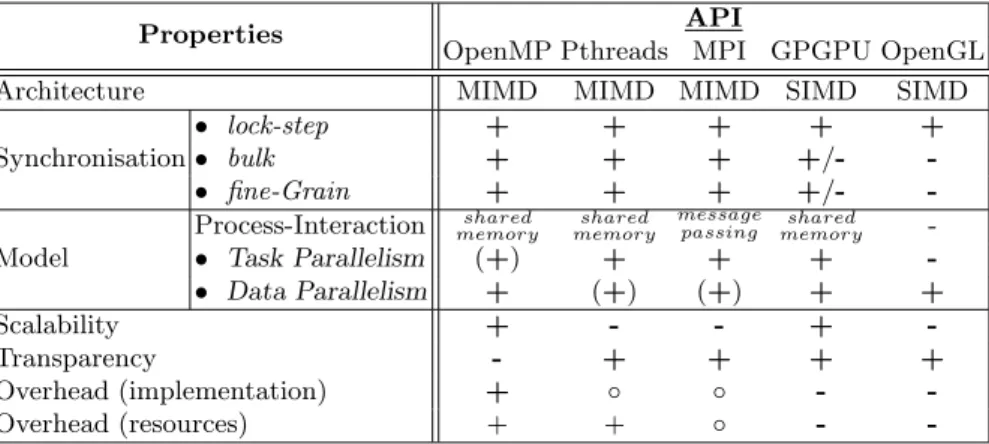
Table 1.Comparison between several techniques for parallel programming
Properties API
OpenMP Pthreads MPI GPGPU OpenGL
Architecture MIMD MIMD MIMD SIMD SIMD
Synchronisation
• lock-step + + + + +
• bulk + + + +/- -
• fine-Grain + + + +/- -
Model
Process-Interaction memoryshared memoryshared messagepassing shared memory -
• Task Parallelism (+) + + + -
• Data Parallelism + (+) (+) + +
Scalability + - - + -
Transparency - + + + +
Overhead (implementation) + ◦ ◦ - -
Overhead (resources) + + ◦ - -
processors are grouped together to form streaming multiprocessors. Program- ming a GPU requires a special compiler, which translates the code to native GPU instructions. The GPU architecture mimics a single instruction multiple data computer with the same instructions running on all processors. It sup- ports different layers for accessing memory. GPUs forbid simultaneous writes to a memory cell but support concurrent reads.
On the GPU, memory is structured hierarchically, starting with the GPU’s global memory called video RAM, or VRAM. Access to this memory is slow, but can be accelerated through coalescing, where adjacent accesses with less than word-width number bits are combined to full word-width access. Each streaming multiprocessor includes a small amount of memory called SRAM, which is shared between all streaming multiprocessors and can be accessed at the same speed as registers. Additional registers are also located in each streaming multiprocessor but not shared between streaming processors. Data has to be copied to the VRAM to be accessible by the threads.
Since frameworks like CUDA have enabled programmers to utilize the in- creased memory and thread management capabilities of modern GPUs, there is a wider selection of applications for GPGPU. Multiple levels of threads, memory, and synchronization provide fine-grained data parallelism and thread parallelism, nested within coarse-grained data parallelism and task parallelism. Thus gradi- ent based mini-batch or even iterative optimization techniques such as SGD may be efficiently run in parallel on the GPU. Regarding flexibility and capabilities GPGPU is positioned between high level parallel programming lnguages such as OpenMP and classical shader programming (see Table 1).
To illustrate the potential of GPGPU programming for machine learning we experimented with a Boltzman machine for solving TSPs [7]. They belong to the class of auto-associative networks that have one layer of neurons. They are completely connected, meaning that changes in activity of a single neuron prop- agate iteratively across the whole network. Boltzmann Machines do not sup- port direct feedback, i.e., a neuron is not connected to itself. Thus, in principal
auto-associative networks are no neural networks. A Boltzmann Machine is in- herently parallel and thus we obtained a 487-fold speedup for 30 towns. While the application scales almost linearly on the GPU, it scales exponentially on the CPU. For more than 120 consumption exceeds the limits of the grapics device.
We encapsulate data fields that needs to be copied between CPU and GPU to minimize the number of data transfers and to store the data in the order in which it is accessed by the threads. Size and indices of data fields are encapsulated and data fields are buffered since older GPU architectures only support 32-bit words.
The indices are stored in 1-dimensional texture memory, since this contains a cache even in older GPU architectures and every thread frequently accesses the indices. Besides, this reduces memory complexity because data is conglomerated in a buffer and thus data transfers are handled in one single transaction. If required it is also possible to just copy single data fields of arbitrary size.
Concerning the infrastructure, the running time is evaluated with functions from the NVIDIA CUDA Event API. It guarantees precise measurements even if the program execution is handed to the GPU for several seconds for synchronous calls in the worst case. The GPU (GeForce GTX 470) of the experiments has been overclocked by Zotac. It contains 14 streaming processors. Since the warp size is currently 32, there will be at most 30·14·32 = 13440 concurrent threads at a time on the chip that will be executed with a shader clock frequency of 1215 MHz. The memory size (1280 MB) is sufficient for all data sets that are used in this work. As opposed to older GPUs its shared memory size is 64 KB (older architectures normally have 16 kilobyte of shared memory) and supports atomic floating point arithmetic. The CPU (i5-7502) from Intel has 2.66GHz clock frequency and 8192 KB Cache. The operating system was Ubuntu 11.04 32 bit. Dependent on the algorithm and its input data it was necessary to close the X-server before running the program. We used Valgrind as a profiling tool to identify the parts of the application with a high arithmetic complexity.
3 Stochastic Gradient Descent and Parallelization
SGD approximates the true gradient for each new training example by θ = θ−ηN
i=1∇L(θi), whereθis a weight vector,η is the (adaptive) learning rate andLis some loss function. SGD is inherently sequential and tends to converge to local minima for non-convex problems. As a compromiseθ may be updated by mini-batches, consisting of the sum of several training examples. The idea of mini-batches complements the semi-parallel CUDA programming paradigma
SGD converges to a good global solution, while the parallel computation of the gradients is likely to produce poor results because the parallel processing of the input data has the negative side effect that threads do not profit from and even more do not consider the changes in the objective that other threads are performing at the same time. A hybrid approach is to use the non-optimal parallel solution to rapidly converge to some adequate solution and than further improve this solution by using the CPU-based solution. This approach combines the shorter execution time for one training iteration on the GPU with the better
precision on the CPU. The time for data transfer alone often exceeds the com- plete CPU-based training time. Therefore, it is necessary to also implement the validation on the GPU. Although the validation only requires reading access, we adopted the memory access pattern from the training procedure.
Bottou [1] states that SGD is well suited for SVMs because the problem is based on a simple convex objective function. This also applies well for CF.
Even for SVMs we found that almost 70% of the CPU instructions are used for vector addition and scalar products, an indicator that the application might benefit from GPGPU. But since the vector length is most often limited to a few dozen elements, standard functions such as those from the CUBLAS-library are practically inapplicable. The input data is already provided as support vectors, which are used to fixθ in each episode. Since the vectors lengths vary greatly, they cannot be simply partitioned on thread blocks with a fixed number of threads. Additionally each training episode requires numerous memory accesses toθ that do not exhibit spatial locality which could be efficiently exploited by the VRAM-controller. As a solution to this problem, θ might be loaded into shared memory. Considering the limited shared memory size of only 64KB the training data has to be loaded piecewise and a hash function has to be defined so that every thread may infer its input data from its thread ID. In other words the hash function allows a block of threads to load exactly those elements ofθinto shared memory which are needed for the training data that has been assigned to this block.
4 Application: Collaborative Filtering
Matrix Factorization for CF is based on the idea that any matrixR ∈RN×M with ratings can be approximated by a matrix P ∈ RN×K of user IDs and a matrixQ∈RK×M with article IDs: R≈P Q. HereN is the number of users, M is the number of articles andK is the number of parameters, that are used to characterize those. The bigger one chooses K the more precisely R can be approximated. This approach holds the advantage to generalize to non-existent ratings based on two low-dimensional matrices. Tak´acs et al. [11] calculate the prediction error by
eui=1
2((rui−rˆui)2+λpTupu+λqTiqi), (1) whereruiis the actual rating, ˆrui the prediction andλis a regularization factor.
Thus the gradient may be calculated by
∂
∂pukeui=−eui·qki+λ·puk (2)
∂
∂qkieui=−eui·puk+λ·qki (3) and therefore the SGD update rule in each step for userpuk and movieqkiis:
puk=puk+ηp(u, i, k)·(eui·qki−λp(u, i, k)·puk) (4) qki =qki+ηq(u, i, k)·(eui·puk−λq(u, i, k)·qki). (5)
To compare the SGD to a batch optimization we also implemented an Alternat- ing Least Squares optimization on the GPU where the update step is basically pu =Wudu, where du denotes the input-output covariance vector and Wu is the updated inverted covariance matrix of input.
Although solving this least squares problem normally involves matrix inver- sion, Koren et al. [6] developed an update rule that is based on the Sherman–
Morrison formula and only shows quadratic complexity.
The idea is to adjust the inverted covariance matrix in each step to the new training example rather than completely recalculate it.
Wu=Wu−(Wuqi)⊗(qTi Wu) 1 +qTi Wuqi
(6) du=du+qi·rui (7) This technique is also based on matrix factorization but yields the advantage that P andQare alternately being updated so that eitherP orQcan be treated as in- or output and be written in parallel.
Fig. 4 shows that first of all P andQ are being compressed to the required dimensions. Afterwards a hash functionφis being created that maps every user to the movies he has rated. Thus multiple threads can simultaneously process the
Fig. 1.Control flow in Collaborative Filtering
ratings by one user in a shared memory. Next the training data is transferred to the GPU and the optimization is being performed. Batch (ALS) and mini-batch (ASGD) optimization need an extra step to load the data into shared memory.
As application we choose the Netflix-competition that was finished in 2009 and awarded the winners with one million US-Dollar. First of all, Netflix provided with over hundred million user ratings the biggest real data set for collabora- tive filtering so far. Secondly, during the competition many interesting machine learning techniques have been developed. Two of them, both based on matrix factorization, will be accelerated by the GPU in this work. Netflix is an on- line DVD rental agency, which uses an AI-based system to recommend movies to users based on their previous purchases. The system that Netflix used until the conclusion of the competition on September 21st in 2009 had a root mean squared error (RMSE) of 0.95256. The RMSE is defined as follows (τ denotes the training set):
RM SE=
SSE/|τ |withSSE=
(u,i)∈τ
e2ui =
(u,i)∈τ
rui−
K
k=1
pukqki
2
T¨oscher et al. [12] won the competition with a final RMSE of 0.8554. They used (amongst others) an estimator calledBiased Regularized Incremental Simulta- neous Matrix Factorization (BRISMF). It has been introduced in 2008 in the context of a progress report for the Netflix competition. It also uses SGD. We re- implemented BRISMF for the GPU, Fig. 2 shows the profile of time vs. accuracy for our implementation of BRISMF using the netflix data.
Before measuring the RMSE for the first time we train the model once with the complete training data set which is why the RMSEonlyimproves by about 10 percent afterwards. This first training episode is also the reason why the curves do not start at time zero. We see that the naive parallelization gives good results. The error (0.9101) is slightly bigger than the original one (0.9068), on
Fig. 2.BRISMF time-accuracy trade-off forK= 40
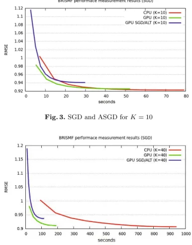
Fig. 3.SGD and ASGD forK= 10
Fig. 4.SGD and ASGD forK= 40
the other hand we measure a speedup of 1088/180 = 6.04. It should be noted that the overall precision for both programs increases if we increaseK.
The comparison between SGD, ASGD and ALS in Fig. 3 shows, that alter- nating SGD yields the worst results. Although ASGD shows a 80/30≈2.66-fold speedup and gives always the same results, it converges to 0.941, as opposed to 0.922 for SGD on the CPU (forK= 10). While a greater value for K gives up to 9-fold speed-up, Fig. 4 shows that the precision remains on a clearly lower level.
5 Application: Support Vector Machine
Raw data presented to a supervised statistical machine learning algorithm [10]
is often mapped to a set of numerical values, called the feature vector. The classification problem deals with the prediction of the labels l of previously unknown feature vectorsx∈Rd that constitute the test data. During training,
Fig. 5.Control flow in SVM training
a partitioning of the feature spaceRdis learned, where each partition is assigned a label based on a set of training samples with known label. The challenge is to approximate the unknown distribution without overfitting the training data.
Support Vector Machines [13] achieve this task by learning coefficients for a kernel mapping to a high-dimensional space, where a linear class border is spanned up by a number of support vectors that outline the data.
We keep the presentation brief as there are text books on SVMs and related kernel methods [4,9]. Theoretically, it should be sufficient to determine the class border by just three support vectors. However, it is not known in advance if any of the known kernels realises a suitable mapping. The use of generic kernels instead leads to a much larger number of support vectors (which critically influ- ence classification time). In the worst case finding a separating hyperplane takes quadratic time in the number of data points.
Leon Bottou [1] uses a SVM to classify text documents. He applies stochastic gradient decent for training and classifying wrt. a linear SVM. This state-of- the-art already gives good results after a very short time (order-of-magnitudes speedup) compared to other libraries, like SVMLight or SVMPerf2. The gradient update rule for an observationxand corresponding classificationy is given by
2 http://leon.bottou.org/projects/sgd
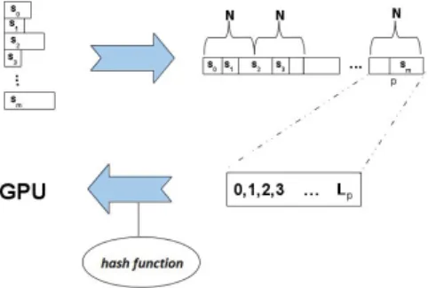
Fig. 6.A hash function to map input to threads during parallel execution
θt+1=θt−ηt∇(xi(t), yi(t);θt)−ηt· ∇r(θt), (8) where θ is the weight vector, ηt is the learning rate at time t, ∇ is the first derivative, is some loss function andi(t) is some random index. The error on the validation data can be checked by summing over all misclassifications:
Number of errors =
i
1, if yi(θ·xi−b)<0
0, else. (9)
The control of flow is shown in Fig. 5. The compression of the input vectors in Fig. 6 is implemented with an STL-vector and has been accelerated with OpenMP. While the support vectors vary in length and are scattered acrossθ, the hash function sorts the input data so that every block of threads processes an equal amount of spatially correlated input data. The hash is like a register that enables each thread to map its input to the global weight vector. This is significantly more efficient on the GPU than transferring the indices itself for each thread, because this would double the size of input data. Creating the hash and resorting the input data is implemented with arrays since dynamic data structures like lists are too slow and would over-compensate the speedup from the following calculation ofφ.
int n = 0 ;
for ( i d = min ; i d < max ; ++i d ) { w e i g h t = i n p u t [ i d ] ;
i f ( ha sh [ w e i g h t ] . map >= |θ|) ha sh [ w e i g h t ] . map = n++;
o u t p u t [ i d ] = ha sh [ w e i g h t ] . map ; }
To speed up the data transfer, floating point numbers are compressed to 16- bit integers on the CPU via the OpenEXR3-library and extracted on the GPU via half2float, which is very accurate especially for input values near zero
3 http://www.openexr.com
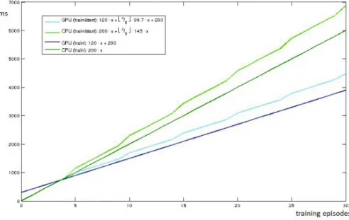
Fig. 7.SVM episodes on GPU/CPU with and without validation
and does not affect the overall precision. Threads collaborate block-wise during training. At first all of the weights, which are required by the threads, are loaded into shared memory. Then comes a thread barrier. Finally each of the thread processes adds the delta to the shared memory. The mapping of shared memory into global memory is implemented by the hash function. Afterwards there is another thread barrier before the threads collaboratively write the delta from the shared memory to the global memory, i.e. add it toθ. Loading the data works analogous for the validation. Each thread checks for the correct classification and adds one to the global error counter in case its wrong. The training data size is substantial (≈ 350MB). Since training takes only about 1.4 seconds and the training data must be first of all uploaded to the GPU, the best possible speed-up is limited. The results with/without cross validation are shown in Fig. 7. It shows that training on the CPU is faster for up to four training episodes because of the initial computational overhead for creating a hash function and transferring data to the GPU. After five episodes the combined training and validation is faster on the GPU.
6 Concluding Remarks
In this paper we showed, that GPUs are already suited to accelerate machine learning techniques with gradient decent. We used different optimization tech- niques to minimize the memory requirements on the GPU and were able to process hundreds of megabytes on the GPU efficiently. Momentarily, parame- ters have to be adjusted sometimes to the specific GPU architecture, although
this is likely to change in the future. We tested local as well as global gradients and compared speed, precision and scalability of each method. We were able to accelerate BRISMF by a factor of 6 while SVMs showed a 1.66-fold speedup.
References
1. Bottou, L.: Stochastic gradient SVM (2010),
http://leon.bottou.org/projects/sgd#stochastic_gradient_svm 2. Carpenter, A.: cuSVM: a CUDA implementation of SVM (2009),
http://patternsonascreen.net/cuSVMDesc.pdf
3. Catanzaro, B., Sundaram, N., Keutzer, K.: Fast support vector machine training and classification on graphics processors. In: ICML, pp. 104–111 (2008)
4. Cristianini, N., Shawe-Taylor, J.: An Introduction to Support Vector Machines and Other Kernel-based Learning Methods. Cambridge University Press (2000) 5. Kato, K., Hosino, T.: Singular value decomposition for collaborative filtering on a
GPU. Materials Science and Engineering 10(1), 12–17 (2010)
6. Koren, Y., Bell, R., Volinsky, C.: Matrix factorization techniques for recommender systems. Computer 42, 30–37 (2009)
7. L-Applegate, D., Bixby, R.E., Chvatal, V., Cook, W.J.: The Travelling Salesman Problem. Princeton University Press (2006)
8. Platt, J.C.: Sequential minimal optimization: A fast algorithm for training support vector machines (1998),
http://research.microsoft.com/pubs/69644/tr-98-14.pdf 9. Schoelkopf, B., Smola, A.J.: Learning with Kernels. MIT Press (2001)
10. Summa, M.G., Bottou, L., Goldfarb, B., Murtagh, F., Pardoux, C., Touati, M.
(eds.): Statistical Learning and Data Science. Chapman & Hall (2011)
11. Tak´acs, G., Pil´aszy, I., N´emeth, B., Tikk, D.: Matrix factorization and neighbor based algorithms for the Netflix Prize problem. In: ACM Conf. on Recommendation Systems, pp. 267–274 (2008)
12. Toescher, A., Jahrer, M., Bell, R.M.: The bigchaos solution to the Netflix Grand Prize (2009)
13. Vapnik, V.N., Chervonenkis, A.Y.: Theory of Pattern Recognition. Nauka, USSR (1974) (in Russian)
14. Zastrau, D.: Beschleunigte Maschinelle Lernverfahren auf der GPU (2011), http://anonstorage.net/PStorage/74.diplomarbeit-david-zastrau.pdf