Force eld molecular dynamics at high hydrostatic pressures: Water, osmolytes, and peptides

Force eld molecular dynamics at high hydrostatic pressures: Water,

osmolytes, and peptides

Dissertation

zur Erlangung des Doktorgrades der Naturwissenschaften (Dr. rer. nat.) der Fakultät für Chemie und Pharmazie

der Universität Regensburg

vorgelegt von Christoph Hölzl

aus Ingolstadt

im Jahr 2018

Abstract

Understanding water and aqueous solutions of biomolecules at high hydrostatic pressure is important not only for the research of deep sea life, but also for gaining insight into properties relevant to ambient conditions. Some small organic molecules, called osmolytes, can stabilize or destabilize the native conformation of proteins in cells against external stresses like temperature and pressure. We use force eld molecular dynamics simulations to study the inuence of selected osmolytes on water and proteins solutions with respect to their response to high hydrostatic pressure. This is achieved using dierent approaches, which are aimed to lay the foundations for understanding and being able to simulate osmolytes at high pressures and then applying these fundamental results to more realistic systems:

1. We present a detailed analysis of the structure of pure water close to a hydrophobic alkane monolayer, which serves as a model system for studying hydrophobic solva- tion, up to 10 kilobars of pressure. The structural properties of interest include the frequency and geometry of rings in the hydrogen bond network, from which we de- duce that the instantaneous structure of water at this hydrophobic interface increases its likeness to hexagonal ice with increasing pressure.

2. We show that it is necessary to modify the force eld parameters of the protecting osmolyte trimethylamine-N-oxide (TMAO) in order to correctly reproduce its solva- tion structure at high pressures, and we present a systematic procedure for scaling the partial charges. For the most relevant protein denaturant, urea, we develop a new force eld for aqueous solutions which signicantly improves upon existing literature models at normal pressure and in the high pressure range.

3. We apply the transfer model to periodic glycine and alanine homopeptides in dif- ferent secondary structures to show that helical conformations of these peptides are stabilized by TMAO even at 5 kilobars relative to an extended structure.

4. We simulate folding of the Trp-cage miniprotein in water and in TMAO solution

at normal and high pressures. We nd some evidence that the protecting eect of

TMAO on the tertiary structure of Trp-cage is weaker but still present at 10 kbar.

Glossary

Acronyms

aiMD ab initio molecular dynamics CD circular dichroism

EC-RISM embedded cluster reference interaction site model

force eld

H-bond hydrogen bond

KBI Kirkwood-Bu integral (

)

LJ Lennard-Jones

MD molecular dynamics OTS octadecyltrichlorosilane PDB Protein Data Bank PMF potential of mean force

QC quantum chemistry

RDF radial distribution function

RMSD root mean squared deviation SAM self-assembled monolayer SASA solvent-accessible surface area TFE transfer free energy

TMAO trimethylamine-N-oxide vdW van der Waals

Symbols

dielectric constant

i

parameter in the LJ potential of atom type

(unit: kJ/mol)

Kirkwood-Bu integral (KBI)

probability or probability density

p

system pressure

q_3/4

tetrahedral/trigonal-pyramidal order parameter

point charge

ρ

mass density

r position vector

radius of gyration

ρi

number density of component

σi

parameter in the LJ potential of atom type

(unit: nm)

T

Temperature

U

potential energy

V

volume of the simulation box or subbox

partial molar volume of component

ring twist

y_i

activity coecient in the molarity scale

Contents

1. Introduction 1

2. Methods and fundamentals 5

2.1. Simulation details . . . . 5

2.2. Hydrogen bonds . . . . 6

2.3. Kirkwood-Bu theory . . . . 6

2.4. Free energy sampling methods . . . . 9

2.4.1. Umbrella sampling . . . . 9

2.4.2. Temperature replica-exchange MD . . . 10

2.5. Ab initio molecular dynamics . . . 12

2.6. EC-RISM . . . 12

3. Water at hydrophobic interfaces 13 3.1. Methods . . . 13

3.1.1. Simulation Details . . . 13

3.1.2. Contact angle . . . 14

3.1.3. Order parameters . . . 14

3.1.4. Rings in the H-bond network . . . 15

3.2. Results . . . 16

3.2.1. First solvation shell properties . . . 16

3.2.2. Hydrogen bond rings . . . 18

3.3. Conclusions and outlook . . . 27

4. Aqueous osmolyte solutions from ambient to high pressures 29 4.1. Trimethylamine-N-oxide (TMAO) . . . 29

4.1.1. Force eld overview . . . 29

4.1.2. Methods . . . 30

4.1.3. Properties at normal pressure . . . 31

4.1.4. High-pressure adaptation . . . 33

4.1.5. TMAO-TMAO potential of mean force . . . 36

4.2. Urea . . . 37

4.2.1. Force eld overview . . . 37

4.2.2. Simulation methods . . . 37

4.2.3. Solvation structure of existing force elds . . . 39

4.2.4. Force eld optimization procedure . . . 42

4.2.5. Properties of the new force eld . . . 43

4.2.6. High pressure force eld adaptation . . . 50

4.2.7. Urea-urea PMFs . . . 50

4.3. Conclusions and outlook . . . 54

5.5. Conclusions and outlook . . . 68

6. The Trp-cage miniprotein 69 6.1. Methods . . . 70

6.2. Results . . . 70

6.2.1. Secondary structure . . . 70

6.2.2. Radius of gyration . . . 72

6.2.3. C

-RMSD . . . 73

6.3. Conclusions . . . 79

7. Conclusions and outlook 81 A. Hydrogen bond network analysis using graph theory 83 B. Force eld parameters 85 B.1. Bonded potential energy functions . . . 85

B.2. TMAO . . . 85

B.3. Urea . . . 86

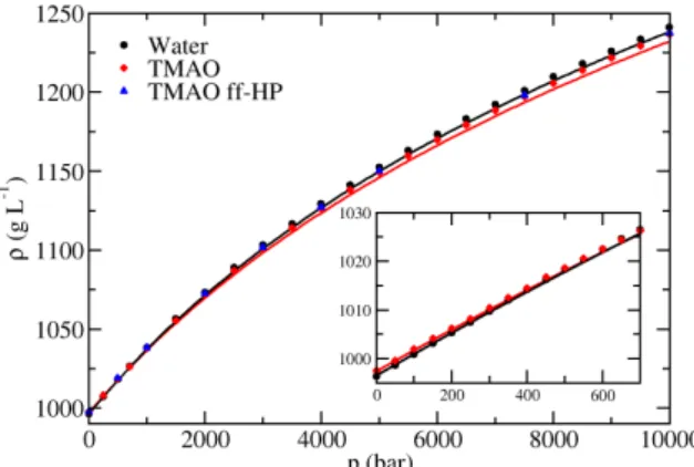
C. Density extrapolation 89

D. High pressure force eld adaptation through individual bond dipole scaling 91

E. Dierential evolution algorithms (DEAs) 93

F. Isothermal and adiabatic compressibilities 95

G. Periodic peptide SASA and TFE data for TMAO solutions 97 H. Conversion between molar concentrations at 1 bar and 5 kbar 99

Bibliography 101

Chapter 1 Introduction

At the time when life rst developed on earth at least 3.5 billion years ago, the conditions on the planet were extreme. It is a distinct possibility that life originated in the deep oceans, e.g. around hydrothermal vents,

where the conditions were still harsh, but more consistent. This means that early life forms must have had mechanisms to protect proteins against these external stresses, since their ability to function is very sensitive to their envi- ronment. Many factors are involved in driving the folding and preventing the denaturation of proteins. Water as the omnipresent solvent plays a major role by driving the hydropho- bic collapse of proteins.

The solvent mixture in the cytoplasm contains a multitude of components that inuence the stability of proteins.

Therefore, it is imperative that we have an understanding of how water and those cosolvents interact with proteins under high hydrostatic pressure. Using pressure as the main thermodynamic variable is not only useful for studying the biophysics of deep sea organisms, but has also become an invalu- able tool for determining properties of biomolecules under ambient conditions, including the equilibrium and dynamics of protein conformations that are relevant to folding and unfolding.

In this thesis, we approach this topic from dierent angles using force eld molecular dynamics simulations. What follows are brief introductions to the individual chapters.

Oil and water are not miscible and form separate phases instead. This phenomenon

is widely known as the hydrophobic eect, but despite making continuous progress,

the

molecular interactions which give rise to the macroscopic eects are still not fully under-

stood. Besides protein folding, hydrophobic interactions with water are important in many

other areas, including the self-assembly of micelles

and other colloidal properties.

There

are multiple systems one has to consider when trying to explain the hydrophobic eect,

since it manifests dierently depending on the size of the hydrophobic particle or phase.

For small hydrophobic molecules, the decades-old theory that water forms an ice-like cage

around the solute

was later refuted, but a moderate slowdown of the water rotational

dynamics was observed in IR spectroscopy experiments

and simulations.

Although it

is now commonly accepted that the solvation shell of hydrophobic solutes is not crystalline

ice, there is evidence that water has certain ice-like properties at some interfaces. Vi-

brational sum-frequency spectroscopy (VSFG) measurements revealed distinct signals for

the stretch vibration of the water O-H bond around antifreeze proteins

and at extended

hydrophobic interfaces.

Water orientations extracted from simulations also support the

view of dangling hydrogen bonds (H-bonds) at simple hydrophobic interfaces consistent

with an ice-like layer.

Since the structure of water is very complex, a wide selection

of parameters has been developed to characterize dierent aspects of water. The simplest

applied to interfaces, and we require dierent methods to identify the structural proper- ties of interfacial water. Water at hydrophobic interfaces has a layer of reduced density, commonly called the hydrophobic depletion layer or 'gap', which has a size on the order of Angströms for alkanes

and peruorinated alkanes.

In previous work we showed that the hydrophobic gap at an octadecyltrichlorosilane (OTS) self-assembled monolayer (SAM) is signicantly compressible.

In chapter 3, we investigate the structure of water at this interface on dierent length scales and quantify its similarity to that of hexagonal ice at dierent pressures.

The term osmolyte refers to the subset of cosolute molecules that exhibit osmotic ac- tivity. It includes many small organic molecules that regulate the osmotic pressure in the cells of all living organisms against external stresses. The group of organic osmolytes includes methylamines, amino acids, sugars, polyols, and urea.

Through evolution, all or- ganisms use a combination of osmolytes that best protects their cells against stresses such as high salinity, temperature, and pressure, while at the same time assuring that these osmolytes are compatible with the cell interior and do not impede the function of proteins in the cytoplasm.

Individually, osmolytes can be separated into two categories: There are osmolytes that protect proteins against denaturation by external stresses, which are called protecting osmolytes or osmoprotectants.

The second category are osmolytes with a destabilizing eect on the native folded state of proteins, commonly called denaturing osmolytes. The most commonly studied protecting osmolyte is trimethylamine-N-oxide (TMAO), because it is one of the most eective protecting agents against protein denatu- ration by temperature, pressure, and denaturing osmolytes.

Currently, there is no full consensus about the molecular mechanism by which TMAO stabilizes proteins. Zou et al.

suggest an indirect mechanism in which TMAO alters the water structure around proteins

by strengthening water-water H-bonds. Unfolding a protein involves breaking intermolec-

ular H-bonds and forming more protein-water H-bonds, which would require breaking the

stronger water-water H-bonds in the presence of TMAO.

However, there is also evidence

for a direct mechanism in which the exclusion of TMAO from the protein surface leads to

a stabilization of the native protein conformation.

For a detailed discussion of osmolyte

protection mechanisms we refer to a review by Canchi and Garcia.

One extraordinary

eect of TMAO is its protection of proteins against pressure denaturation. It was found

that in salt water sh (specically teleosts), there is a linear relation between the content

of TMAO in the muscle tissue and the shes' native depth.

Out of all denaturing os-

molytes, urea is by far the most relevant in biology, and its denaturation mechanism is now

commonly accepted to be a direct favorable interaction with the protein.

Therefore,

TMAO and urea were chosen as the objects of study and the topic of chapter 4. In nature,

these two osmolytes often occur together in a urea to TMAO ratio of 2:1. The destabi-

lizing and stabilizing eects of both components are additive and approximately cancel

out, which means this mixture can be used in high stress environments in adequately high

concentrations without interfering with protein function.

In this thesis, the main

focus lies on using pressure as a variable to better understand the eect of osmolytes on

proteins and water. While there are experimental studies on osmolyte eects on the pres-

sure denaturation of proteins and peptides,

simulations are signicantly hindered by the fact that force eld approaches are dependent on sets of parameters that have not been validated outside of ambient conditions, whereas ab initio methods are too expensive even for small peptide systems. Chapter 4 exclusively deals with binary osmolyte/water mixtures of TMAO and urea. We introduce the necessary modications to an existing TMAO model for simulations at high pressure, and we fully develop a new force eld for urea which performs well under ambient and high pressure conditions.

Our main interest in osmolytes is the study of their molecular-scale protein denaturation and stabilization mechanisms. Recently, a simulation study of the folding/unfolding equi- librium of a hydrophobic model polymer has shown that the stabilizing eect of TMAO may not monotonically increase with TMAO concentration, but that TMAO could even fa- cilitate the unfolding of hydrophobic polymers at very high concentrations.

In chapter 5, we apply the tools developed in the previous chapter to study the eect of TMAO concen- tration and pressure on the stability of dierent helical structures of model homopeptides of glycine and alanine.

One of the main long-term goals of molecular dynamics simulations is gaining the ability

to study the folding process of proteins. This is not only relevant to understanding their

biophysical and biochemical functions in nature, but also to gain insight into the origin

and ramications of folding defects, which are believed to cause diseases such as cystic

brosis

and Alzheimer's.

It was found that protecting osmolytes such as TMAO can

prevent folding defects,

which raises the question whether this eect diers from the

molecular mechanism by which these osmolytes stabilize against temperature and pressure

denaturation. The main challenge for simulations are the timescales on which most proteins

fold, which is usually on the order of milliseconds. Immense eort has been put into

designing the fastest-folding protein, which resulted in the 20-residue Trp-cage miniprotein

TC5b

with a folding time on the order of 4

s.

It has already been intensely studied as a

prime model system for globular proteins using experiments and simulations in water as well

as osmolyte solutions.

The interplay of urea and pressure on Trp-cage stability has

been investigated using replica-exchange MD (REMD) simulations

and, more recently, a

combination of high-pressure NMR spectroscopy and simulations.

However, the studies

combining TMAO and Trp-cage have so far been limited to normal pressure conditions.

In chapter 6, we present results of folding simulations in TMAO solutions at ambient and

high pressures.

Chapter 2 Methods and fundamentals

2.1 Simulation details

All simulations in this work were performed using the following methods, unless they are explicitly mentioned in the methods section of a subsequent chapter. For the molecular dy- namics (MD) simulations the GROMACS program package with versions ranging from 4.6.5 to 2016.4 (all compiled in single precision) was used. In molecular dynamics, Newton's equa- tions of motion of a many-body system are numerically integrated using a nite dierence method, in this case the leap-frog algorithm. In our nonpolarizable force eld MD simula- tions, all interactions are described by analytical two-body potentials. The Lennard-Jones (LJ) potential models the van der Waals interactions (eq. 2.1):

U_ij^LJ(r_ij) = 4_ij

"

σ_ij rij

12

− σ_ij

rij

6#

(2.1) Here

and

are the two particles,

is the variable distance between the two particles, is the potential minimum depth, and

is the distance where the potential vanishes. We use the Lorentz-Berthelot combination rules to calculate

and between dierent atom types:

σ_ij = σ_i+σ_j

2

(2.2)

ij =√

i·j

(2.3)

For electrostatic interactions we use the Coulomb potential. The LJ interactions and the real-space Coulomb interactions were cut o at 1 nm, and the long-range electrostatics was computed using smooth particle-mesh Ewald summation

with a lattice spacing of 0.12 nm. In isotropic systems, the eect of a nite LJ cuto range was accounted for using a long range dispersion correction for the energy and virial as implemented in GROMACS.

In order to simulate thermodynamic ensembles other than the microcanonical (N V E)

ensemble, thermostat and barostat algorithms were applied. For temperature control, the

stochastic velocity rescaling algorithm (sometimes called 'canonical sampling through ve-

locity rescaling' or CSVR)

was used with a time constant of 1 ps to x the temperature to

300 K. For pressure control, two barostat methods were used: The Berendsen barostat,

which does not reproduce the correct pressure uctuations of the

ensemble, was ap-

plied in equilibration simulations with a time constant of 1 ps, since it relaxes the system

volume to its equilibrium value very quickly. The Parrinello-Rahman barostat

does con-

measures.

2.2 Hydrogen bonds

The way we determine hydrogen bonding in our simulations is based on a purely geometric criterion. A variety of such H-bond denitions have been used in the literature, which will not be discussed here.

We use a relatively new criterion introduced in ref. 64. This criterion has been proven to properly identify H-bonds in water at high pressures up to 10 kbar. An H-bond is dened to exist when

rH···A<−0.171 nm·cos (θD−H···A) + 0.137 nm

(2.4) where D and A are the donor and acceptor atoms respectively,

is the distance between the donated hydrogen and the acceptor, and

is the angle between the donor- hydrogen bond and the hydrogen-acceptor vector.

2.3 Kirkwood-Bu theory

In their theory of mixtures,

Kirkwood and Bu derived relationships between the ra- dial distribution functions (RDFs) and the particle number uctuations for solutions in the grand canonical

ensemble. The uctuations were then related to macroscopic thermodynamic properties such as the derivative of the chemical potential, partial molar volume, and compressibility, thus establishing a direct connection of the integrals over the RDFs, hereafter called Kirkwood-Bu integrals (KBIs), and the thermodynamics of the system. In this work we apply Kirkwood-Bu theory only to binary mixtures, and we will use the notation and relations found in ref. 66. The KBI

is dened in eq. 2.5:

G_ij = Z ∞

0

4πr²h

g_ij^{µV T}(r)−1i

d

(2.5)

Here,

is the distance between the centers of mass of molecules of type

and

, and

is the RDF of the two components in an open system with constant volume and temperature.

In a binary mixture of molecules

and

, the thermodynamic properties can be expressed using the auxiliary quantities

and

:

η=ρ_A+ρ_B+ρ_Aρ_B(G_AA+G_BB−2G_AB)

(2.6)

(2.7) Here

are the number densities of the components. The partial molar volumes are then

V¯_A= 1 +ρ_B(G_BB−G_AB)

η

(2.8)

V¯B = 1 +ρA(GAA−GAB)

η

(2.9)

2.3. Kirkwood-Bu theory and the isothermal compressibility can be calculated as

κ_T= ξ

k

(2.10)

We also obtain the density derivative of the chemical potential of the components

∂ρA

p,T

=

k

ρA(1 +ρAGAA−ρAGAB)

(2.11) where

and

are pressure and temperature, and k is the Boltzmann constant. Since we will specically be dealing with activity coecients in the molarity scale

, we use the following expression for the logarithmic derivative of the activity coecient of component

with respect to the number density (or molar concentration) of component

y_AA=

∂

ln

∂

ln

p,T

= ρ_A(G_AB −G_AA)

1 +ρ_A(G_AA−G_AB)

(2.12) While this theory is incredibly useful, its practical application in simulations suers from one major problem: It is only exact for the RDFs in the grand canonical ensemble. Al- though it is possible to simulate this ensemble directly using e.g. grand canonical Monte Carlo, this method is severely limited in its application to low densities since the molecule insertion moves during the simulation need to have a reasonably high probability.

Instead, it is common practice to simulate the system of interest in the

or

ensembles.

The obtained RDFs are then empirically corrected to account for the dierences between the ensembles outside of the thermodynamic limit. The simplest correction is to integrate eq. 2.5 up to a nite distance, and assume that

for larger distances. This way the divergent integral is assigned a nite value. Other ad-hoc corrections are the shift or division of the whole RDF by the dierence of the long-range limit of

from unity. A more sophisticated method uses the argument that, in a closed system, a local excess of particles causes a depletion elsewhere.

Recent progress has been made by combining this correction with a dierent one, which resulted in the best convergence of KBIs obtained from RDFs so far.

In this work we use a dierent approach developed by Cortes-Huerto et al.,

which forgoes the use of RDFs and uses the relationship between the KBIs and the particle number uctuations:

Gij =V

hN_iN_ji − hN_iihN_ji hN_iihN_ji − δ_ij

hN_ii

(2.13)

is the volume of the system,

are the average particle numbers, and

is the Kronecker delta. This relation is also only valid for an open system. In practice, we calculate the uctuations in a subvolume

inside the simulation box with xed

and total volume

. The KBIs of the subsystem are then a function of both

and

:

Gij(V, V0) =V

hN_iN_ji_V,V0 − hN_ii_V,V0hN_ji_V,V0

hN_ii_V,V0hN_ji_V,V0 − δij

hN_ii_V,V0

(2.14) All the particle number averages now depend on both the volume of the system and that of the selected subbox. The authors then derive a relation between the KBIs in the subbox and in the thermodynamic limit

:

Gij(V, V0) =G^∞_ij

1− V V0

− V δ_ij V0ρi

+ α_ij

V¹³

(2.15)

λ=

V0

(2.16)

and multiplying eq. 2.15 with

−λ⁴δ_ij ρ_i + α_ij

V

1 3

0

(2.17)

In the region of

this reduces to

λGij(λ) =λG^∞_ij + αij

V

1 3

0

(2.18) which is linear in

. We can now calculate

from one simulation with volume

by analyzing subboxes with dierent volumes. From the intercept of the linear t of

we obtain

, and the slope gives us the KBI in the thermodynamic limit

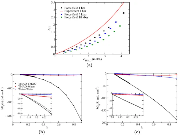
. As an example, g. 2.1 shows

directly calculated from eq. 2.14, and the function in eq.

2.17 using the parameters obtained from the linear t.

In our implementation of this method, the KBIs of multiple subvolumes are calculated and then averaged for each

value. The placement of the subboxes is either random or on a regular grid, where the subboxes can overlap and wrap around the periodic boundaries of the system. For all results in this work, we use the grid method with 512 subboxes per

value, although the subbox placement does not inuence the KBIs within the uncertainties as long as the system is suciently sampled. The

range for the linear t needs to be adjusted depending on the total system size. For a box with edge lengths of

nm we use

for aqueous urea solutions and

for TMAO solutions.

Adjustments may be necessary depending on the solute and box size.

Figure 2.1.: Example for the KBI calculation method in ref. 70: λGij(λ) of the three possible combinations of species in a 2 mol/L aqueous TMAO solution (results taken from section 4.1). The symbols are the values calculated from the uctuations (eq. 2.14), and the lines are eq. 2.17. G^∞_ij andαij are determined from a linear t in the range 0.1≤λ≤0.3 (the range shown in the inset). For eachλ, eq. 2.14 was evaluated for 512 subboxes placed on a grid, and then the average over the subboxes was taken.

2.4. Free energy sampling methods

2.4 Free energy sampling methods

2.4.1 Umbrella sampling

We are often interested in the free energy

of a system. It is dened in statistical thermodynamics as

F =−β⁻¹

ln

(2.19) where

k

, k is the Boltzmann constant,

the temperature,

the canonical partition function, and

the number of particles in the system. Unfortunately,

is an integral over the

-dimensional phase space, which is impossible to solve even for moderately large

:

Q= 1 N!h^3N

Z

d

d

(2.20) with the Planck constant

, the Hamiltonian

, and the

-dimensional position and momentum vectors

and

of indistinguishable particles, which is the origin of the prefactor

(which would be dierent for other system compositions).

Although the free energy is not directly accessible, it is possible to calculate dierences in free energy along a chosen reaction coordinate, called the potential of mean force (PMF).

Ref. 71 gives an introduction to free energy methods in general, and umbrella sampling in particular, which we will summarize in the following section. The partition function can be written as a function of any reaction coordinate

:

Q(ξ) =

R

d

R

d

(2.21)

δ

is the Dirac delta distribution. Here the momenta

were integrated out, and all pre- factors were discarded, since they are an additive constant in the free energy and we only care about dierences along

is the potential energy, which is assumed to only depend on the positions. In principle, one could run a regular MD simulation to sample the whole range of

and calculate the free energy dierences from the probability distribution of

sampling of free energy barriers along the reaction coordinate. In umbrella sampling, which was developed by Torrie and Valleau,

an articial bias potential

is added to the unbiased potential energy

of the system:

U^b(r) =U^u(r) +w_i(ξ)

(2.22) The index

refers to one specic bias potential, which samples one region of

space, usually called a 'window'. The most common bias potential is harmonic, which we use throughout this work:

wi(ξ) =

K

2(ξi−ξ)²

(2.23)

ξi

is the equilibrium position for the reaction coordinate in window

constant.

The probability distribution of

in a window is a biased distribution

. The unbiased

free energy of this window can be calculated except for the free energy term

, which is

independent of

(see ref. 71 for details):

weights

by which the individual unbiased

are scaled to minimize the total variance of the global unbiased probability

P^u(ξ) =

N_windows

X

i=1

pi(ξ)P_i^u(ξ)

(2.25)

From the weights

the constants

can be obtained. But since

depends on

, the

have to be optimized iteratively. Finally, the PMF is calculated:

F(ξ) =−β⁻¹lnP^u(ξ)

(2.26)

We exclusively use the WHAM implementation in GROMACS, which also includes error esti- mates for the PMF.

2.4.2 Temperature replica-exchange MD

When we are interested in sampling high-energy regions of phase space, but there is no simple reaction coordinate, other methods have to be used. One solution is the temperature replica-exchange scheme, which was initially adapted for the use in molecular dynamics simulations by Sugita and Okamoto.

Multiple copies of the same system, the 'replicas', are simulated in parallel at dierent temperatures in the

or

ensemble. For a certain number of simulation steps, the equations of motion of all replicas are propagated independently from each other. Then, at xed intervals, each replica can exchange its temperature with one replica with the next lower or higher temperature. By running this simulation scheme for a suciently long time, a replica stuck in a local free energy minimum will be exchanged to higher and higher temperatures until the free energy barriers can be crossed with signicant probability. In this way the averages and energy landscapes at a certain temperature can be calculated even if the trajectory at one temperature is not continuous and made of short segments of simulations of dierent replicas.

Next, we will briey review the details of this method as laid out in ref. 75. A state

of a number of

replicas is dened as the sets of all positions and momenta for each replica, called

, where the superscript

is the index of the replica, and

is the index of the current temperature of replica

, and there exists a (bijective) map between the two (m

and

xⁱ_m = (

r

p

(2.27)

Here

and

are the

-dimensional position and momentum vectors. A state

is then dened by the

points in phase space

, each of which is assigned to a distinct temperature:

X= (. . . , xⁱ_m, . . .)

(2.28)

As long as the replicas do not interact with each other, the probability

of nding the

2.4. Free energy sampling methods system in state

is just the product of the canonical phase space densities of all replicas:

P(X) = exp (

−

M

X

i=1

β_mH(rⁱ,pⁱ) )

(2.29) At an exchange step, two replicas can exchange temperatures. The state

becomes

:

X = (. . . , xⁱ_m, x^j_n, . . .)

(2.30)

(2.31) Since the exchanged replicas now have dierent temperatures, the instantaneous momenta at the time of the exchange are scaled to be consistent with the kinetic energy at the new temperature:

pⁱ⁰ = rT_n

T_mpⁱ

(2.32)

p^j0 = rT_m

T_np^j

(2.33)

Next it will be described how the probability for an exchange step is determined. The detailed balance condition is assumed, i.e. the exchange probabilities

are that of a system in equilibrium:

P(X)w(X→X⁰) =P(X⁰)w(X⁰ →X)

(2.34) From eq. 2.29, the ratio of the exchange probability to its reverse process can be calculated:

w(X→X⁰)

w(X⁰ →X) = P(X⁰) P(X)

= exp{−∆}

(2.35)

∆ = (β_n−β_m) U(rⁱ)−U(r^j)

(2.36) Here we used the facts that all contributions from replicas not involved in the exchange cancel out, and that the kinetic energy contributions of the exchanging replicas cancel due to the momentum scaling in eqs. 2.32 and 2.33. There are multiple possible choices for

that satisfy this condition. The exchange probability used here is the well-known Metropolis criterion from the Monte Carlo simulation scheme with the same name:

w(X →X⁰) =

(1

if

exp{−∆}

if

(2.37)

This means that if the replica with a lower temperature has a higher potential energy

, the

exchange step is always accepted, and there is a nonzero probability for the exchange oth-

erwise. In this work, we use the GROMACS implementation of the replica-exchange method,

where a replica can only be involved in one exchange attempt at a time. This means that in

alternating exchange steps, a replica is either the low or high temperature in an exchange

attempt. For suciently high exchange probabilities, the potential energy distributions of

neighboring temperatures need to have a reasonably large overlap. We use the method

tained from quantum chemistry. We will therefore use ab initio molecular dynamics (aiMD) simulations performed by Dr. Sho Imoto and Jan Noetzel (refs. 78 and 79) as reference data. Whenever we refer to aiMD in this work, we mean Born-Oppenheimer dynamics simulations performed with the QUICKSTEP module

of the CP2K program package.

The level of theory is density functional theory (DFT) in the generalized gradient approxima- tion (GGA) using the revised Perdew-Burke-Ernzerhof (RPBE) functional

in combina- tion with the D3 dispersion correction.

A detailed write-up of the technical details used in the simulations of a single TMAO in 107 water can be found in ref. 78. The unpublished data for one urea in 110 water

follows the same procedure.

2.6 EC-RISM

In this work, we use results obtained from embedded cluster reference interaction site model (EC-RISM) calculations, which were performed by Patrick Kibies (see refs. 78 and 84). This method combines the reference interaction site model in three-dimensional space (3D-RISM) with a quantum-chemical treatment of a solute molecule to calculate equilibrium properties, e.g. solvent distributions, solvation free energies, and pKa values with chemical accuracy.

One parameter in EC-RISM integral equation theory is the solvent susceptibility, which can in theory be determined directly from molecular dynamics simulations of the pure solvent. However, due to technical reasons, this is currently not feasible in 3D-RISM, and the susceptibilities were instead determined from 1D-RISM using the radial distribution functions from MD simulations. Specically, the results from MD simulations are used in the bridge function term, which is necessary for the closure of the integral equation. The EC-RISM calculation itself is a self-consistent quantum chemistry calculation with the solvent being represented as charges on a grid. The initial charges from 3D-RISM polarize the solute, which in turn changes the optimal solvent charges. This cycle is repeated until self-consistency of the solute and solvent geometries.

All EC-RISM results in this work use solvent susceptibilities extracted from simulations

of SPC/E water

at 298.15 K at various pressures. Currently, the use of four-point water

models (e.g. TIP4P/2005) is not possible for technical reasons. The level of theory was

B3LYP/6-311+G(d,p)/EC-RISM. Dipole moments and partial charges were calculated by

tting the partial charges of the solute to the electrostatic potential of the optimized ge-

ometry using the ChelpG method.

Further technical details of the EC-RISM calculations

for TMAO can be found in ref. 78. The unpublished results for urea

were calculated

analogously.

Chapter 3 Water at hydrophobic interfaces

In this chapter, we perform a detailed molecular-level analysis of the water structure at an alkane self-assembled monolayer (SAM) with pressure as the variable. We present previously published parameters for measuring the local and intermediate-range order of water at interfaces.

For a general introduction to this topic we refer to chapter 1.

3.1 Methods

3.1.1 Simulation Details

The simulations of the SAM/water interface are identical to previous unpublished

and published

work. We modeled the SAM after a SAM of octadecyltrichlorosilane (OTS) on silica, where the silica was omitted since its inuence on the investigated properties is negligible. Instead, the rst carbon atoms of 36 octadecane chains were xed via a freeze group on a hexagonal grid with a lattice constant of

Å, which is the distance between the oxygens of the interfacial silanol-OH groups on silica.

The AMBER03

LJ-parameters were used in conjunction with the OPLS-AA

charges, which introduced the weak electrostatic interactions not present in the AMBER03 force eld. However, we later conrmed that the small partial charges do not measurably inuence the properties studied in this work. The SAM was solvated in 2096 TIP4P/2005 water molecules. The rectangular box had a xed xy-base with measurements of

nm

, and the box length in z direction varied between 10.1 nm at 1 bar (snapshot in g. 3.1) and 8.3 nm at 10 kbar. Semiisotropic Berendsen pressure coupling

with a time constant of 1 ps was used to scale the z component of the box, mainly because using the Parrinello-Rahman barostat

caused unexpected behavior in combination with freeze groups in GROMACS 4.6.5.

The lengths of all bonds involving hydrogen atoms were constrained, which enabled the use of a 1.5 ps time step for integrating the equations of motion. This system was simulated for 210 ns at 300 K and the seven pressures 1 bar, 1 kbar, 2 kbar, 3 kbar, 4 kbar, 5 kbar, and 10 kbar. The SAM/water interface was also simulated for 15 ns at 250 K, 350 K, and 400 K at 1 bar. The trajectory of a simulation of the water/vacuum interface from previously unpublished work

is also analyzed in this work. The system consists of 1073 water molecules in a

nm

slab, which was equilibrated at 1 bar and 300 K.

The box was then extended by adding a 6 nm vacuum phase in the z direction. This system

was simulated in the

ensemble for 210 ns. For the contact angle calculation we also

simulated the SAM in vacuum for 150 ns. Additionally, two bulk ice phases were simulated

using anisotropic Parrinello-Rahman pressure coupling with a 3 ps time constant. An ice

Ih crystal made of 432 water molecules was simulated for 5 ns at 200 K. Using the genice

Figure 3.1.: Simulation snapshots of the SAM/water interface at 1 bar. The snapshot was visu- alized using VMD.⁹⁴

3.1.2 Contact angle

Here, we briey show that our model SAM reproduces the experimental contact angle of water at an OTS SAM on silica. We use Young's equation (eq. 3.1) to calculate the contact angle

from the surface tensions

of the SAM-vacuum, SAM-water, and water-vacuum systems:

cosθ= γ_SAM-vacuum−γ_SAM-water

γwater-vacuum

(3.1)

We chose to calculate the surface tension from the dierence of the lateral and normal pressures (calculated from the virial) in the system integrated over the box length

:

γ= 1 2

Z L_z 0

d

p_zz(z)− p_xx(z) +p_yy(z) 2

(3.2) To avoid the calculation of the prole of local virial tensors, we make the assumption that the dierence between the lateral and normal pressures not only vanishes in the liquid and gas bulk phases, but also in the anisotropic SAM bulk phase. Additionally, we make the approximation that this dierence is constant at the interfaces, which is reasonable if the local pressure dierence has a shape similar to that of the LJ-uid in ref. 95. Then, the surface tension only depends on ensemble averages of the diagonal elements of the pressure:

γ = L_z 2

hp_zzi −hp_xxi+hp_yyi 2

(3.3) Our results for the SAM-vacuum system is

bar

nm, the value for the water-vacuum surface is

bar

nm, and the SAM-water interface has a tension of

bar

nm.

The resulting contact angle of

is in excellent agreement with the experimental value of

.

We therefore assume that our model is a good approximation of the OTS-SAM on silica even without explicitly modeling the substrate.

3.1.3 Order parameters

In this work, we use parameters to quantify the local order around water molecules. The

tetrahedral order parameter

(eq. 3.4) was introduced by Errington and Debenedetti,

which is a modication of the initial order parameter

by Chau and Hardwick.

3.1. Methods

q4(k) = 1−3 8

3

X

i=1 4

X

j=i+1

cos (ψ_ikj) +1 3

2

(3.4)

quanties the angular tetrahedral order of the four nearest water molecules around a water molecule

by summing over the squared deviations of the angles

between two of the four closest water with the central water

combinations out of the four closest neighbors. For simplication purposes, the positions of the oxygen atoms are used as the positions of the water molecules.

is normalized such that it is zero for a random distribution of positions of the nearest neighbors and one for a perfectly tetrahedral coordination (all

).

(eq. 3.5) is dened almost identically to

. The main dierence is that the summation runs only over the three closest neighbors. We changed the normalization factor such that

and

refer to random and tetrahedral angle distributions. With

it is possible to investigate the tetrahedrality of the water network when neighbors are missing, i.e. at an interface.

q3(k) = 1−3 4

3

X

i=1 4

X

j=i+1

cos (ψ_ikj) +1 3

2

(3.5)

3.1.4 Rings in the H-bond network

In this work we apply graph theory to study the hydrogen bond network in water. This approach has already been known since the early days of water simulations.

In recent years, Matsumoto and coworkers used this method to analyze rings in the hydrogen bond network of supercooled water.

We use their method and criterion for detecting rings in the graph.

A detailed explanation of the ring detection algorithm can be found in appendix A.

After all rings are detected, we go back from the abstract graph representation of the hydrogen bond network to the spatial coordinate representation to analyze the geometry of the rings. We use the following denition from ref. 98: A ring has a twist

(eq. 3.6),

χ_R = 1 N

N−1

X

i=0

sin (3θ_ijkl)

(3.6)

where

is the size of the ring, and

are the internal water indices of this ring with

mod

,

mod

, and

mod

.

is the torsional angle

around the H-bond between the water molecules

and

. Figure 3.2 shows the cases where

a single term in eq. 3.6 is zero. The sum over all terms vanishes when all water molecules in

the ring have a perfectly tetrahedral H-bond geometry, e.g. in six-membered rings in chair-

or boat conformation. Alternatively, the nonzero twists can cancel out even in asymmetric

ring geometries.

(a) (b)

Figure 3.2.: View projected along a H-bond for orientations where the torsionsin (3θijkl)is zero.

The lines are H-bonds assuming that each water molecule has four H-bonds. The torsion is zero for both staggered (a) and eclipsed (b) conformations of the H-bonds and takes nonzero values between -1 and 1 otherwise.

3.2 Results

3.2.1 First solvation shell properties

First we will analyze the orientations of water molecules as a function of the distance from the alkane SAM/water interface. We dene the angle

as the angle between the water dipole moment and the surface normal vector which points towards the water phase.

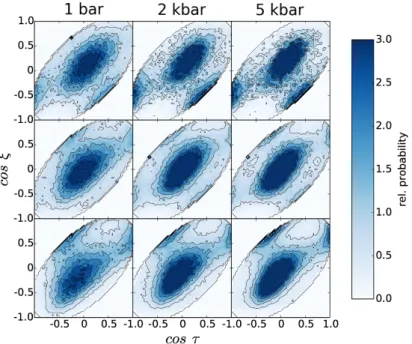
is the angle between the water O-H bonds and the surface normal. Figure 3.3 shows the 2D distributions of

and

normalized to the bulk distribution for pressures from 1 bar to 5 kbar. The distance from the interface increases from the top to bottom rows. Throughout all distributions, the most probable orientation is at

the water molecules are oriented in parallel to the interface. The peaks at

and

closest to the interface mean that one O-H bond points directly towards the interface. Further away from the interface, no preferred orientation besides parallel orientations at

are found. In the next layer, two maxima at

and

emerge. Here, the orientations from the closest layer are inverted such that one O-H bond points away from the interface. Qualitatively, the distributions at all pressures from 1 bar to 5 kbar agree with each other. Only the probabilities of the preferred orientations increase signicantly with pressure, which signies that the water molecules are more strongly ordered at high pressures. The orientations we found are not only consistent with existing literature at normal pressure,

but also with the molecular orientations in a crystal of ice Ih assuming the surface normal is the c axis of the ice crystal. This fact hints at ice-like ordering of water at hydrophobic interfaces which is amplied in a high pressure environment.

In order to further characterize the properties of water at the SAM/water interface, the

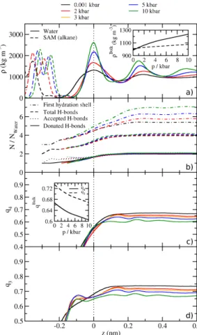
properties of the rst solvation shell of water are analyzed. Figure 3.4 contains laterally

averaged proles of multiple rst-shell properties at the interface. Panel (a) are the mass

densities of the SAM and water components at pressures up to 10 kbar. From the proles

and the bulk densities in the inset it is clear that the SAM is compressed very little

when increasing the pressure from 1 bar to 10 kbar. However, the density of water at

the rst maximum at the interface increases signicantly with this pressure change. Also,

the distance between SAM and the water maximum decreases, which is a result already

found in previous work,

where it was shown that the hydrophobic depletion layer at this

3.2. Results

Figure 3.3.: 2D angle orientations at the SAM/water interface. ξis the angle between the water dipole moment and the surface normal vector (pointing towards the water phase). τ is the angle between the water O-H bonds and the surface normal. The distributions shown here are normalized to the bulk angle distributions. The distributions are shown for pressures increasing from 1 bar (left) to 5 kbar (right). The distance from the interface increases from the top to the bottom panels. At 1 bar, the panels are slices of0.5Å. The slice thickness was scaled with the compression of the box in z direction, leading to 0.465Å slices at 2 kbar and 0.436Å at 10 kbar. The slices in the middle and bottom rows have the coordinate z= 0 in g. 3.4 (dashed line) in common.

Reproduced from ref. 88 with permission from the PCCP Owner Societies.

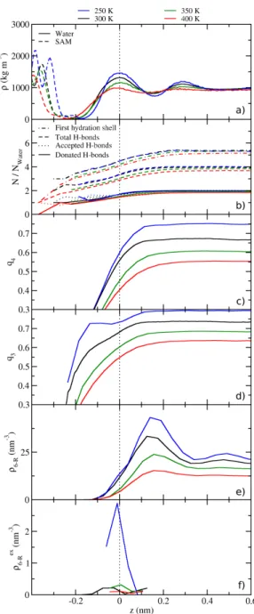
interface is signicantly compressible. In panel (b) we show that the number of water molecules inside the rst hydration shell decreases below four in similar fashion for all pressures, even though the bulk values dier signicantly between 5.3 at 1 bar and 7.0 at 10 kbar. In contrast, the number of hydrogen bonds per water falls o at the interface and is almost identical in bulk and at the interface over the whole pressure range. Only a minor increase at 10 kbar can be observed compared to normal pressure. In conjunction with the number of water molecules in the solvation shell, this means that the majority of the water that is added upon compression is not part of the H-bond network but mostly lls the tetrahedral voids, in agreement with literature.

Directly at the interface, the number of accepted H-bonds is greater than the number of donated H-bonds. This means there are dangling H-bonds at the interface, which agrees with the angle distributions in g. 3.3.

The prole of the tetrahedral order parameter

(eq. 3.4) is shown in panel (c). When the pressure is increased, the bulk value of

decreases. This can be explained by the fact that the water molecules ll the tetrahedral voids in the H-bond network as shown in panel (b). Therefore, the closest four neighbors are less likely to be tetrahedrally coordinated at higher pressures. When approaching the interface,

decreases monotonically at all pressures, since there is no fourth neighbor available at the interface, thereby making a tetrahedral coordination impossible. In order to be able to quantify the tetrahedrality of the remaining three closest neighbors we dene the trigonal-pyramidal order parameter

(eq. 3.5). The qualitative behavior of the bulk values of

in panel (d) is identical to

.

detailed information about the water structure in this system, which will be analyzed in the remainder of this chapter.

Figure 3.4.: Laterally averaged properties of water at the SAM/water interface. (a) The mass densities of the SAM (dashed lines) and water (full lines). The dotted line is a guide to the eye at the position of the rst water maximum. The inset displays the bulk densities of both components as a function of pressure. (b) The number of water molecules in the rst hydration shell around water (dotted and dashed lines), dened as the number of water molecules closer than the minimum of the bulk water-water RDF at 1 bar (0.322 nm). Other data sets are the number of accepted (dotted), donated (dashed), and total (full lines) number of hydrogen bonds per water molecule. (c) The tetrahedral order parameter¹⁸ q₄ (eq. 3.4). (d) The trigonal-pyramidal order parameter q₃ as dened in eq. 3.5. The inset in (c) shows bulk values forq₄ andq₃.

3.2.2 Hydrogen bond rings

After investigating the rst-shell solvation properties at the SAM/water interface, the

structure of water at an intermediate range will be analyzed. In this section, we describe

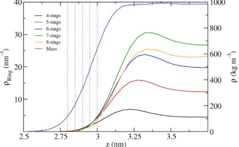
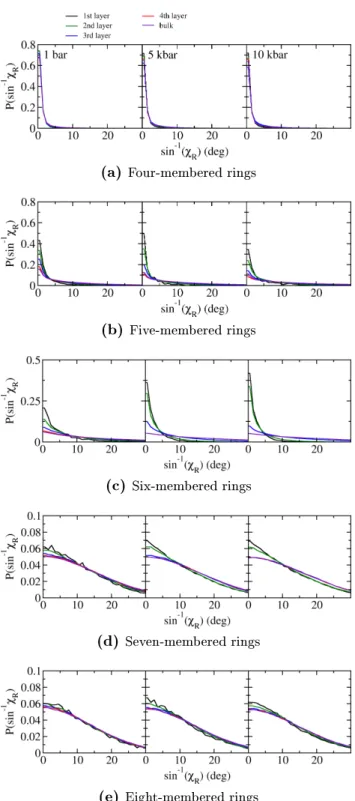
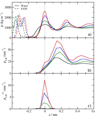
3.2. Results the topology of the H-bond network, specically rings formed by H-bonded water molecules as dened in sec. 3.1.4. First the results for four- to eight-membered H-bond rings at the vacuum/water interface are presented, which serve as a reference for the SAM/water results. Figure 3.5 shows that the density proles of the rings of all sizes assume a maximum in the vicinity of the interface. These maxima are not correlated to the mass density of the water phase. For four- to seven-membered rings, an increase of the absolute ring densities is observed over the whole coordinate range. The eight-membered ring density prole takes values between six- and seven-rings in bulk and decreases to the lowest density out of all observed ring types close to the interface. In bulk, the densities range from

four-membered rings per nm

and

nm

seven-rings. Although signicantly larger ring sizes can also be observed, their data contained no meaningful information and is not shown. Next, the geometry of the rings is analyzed. As a measure we use the twist of a H-bond ring

as dened in eq. 3.6, which determines how distorted the ring geometry is.

Therefore, the twist is a measure of the 'tension' of the H-bonds in the ring. In g. 3.6, the distribution of

is shown for multiple layers of water close to the interface. The region we investigated is much closer to the vacuum phase than the ring density maximum and has a mass density signicantly lower than the bulk. The twist distributions of four-membered rings are very narrow and centered around

. Only a very minor decrease of the twist is observed when going from the interfacial region to the bulk phase. This is due to the limited exibility of the H-bonds before a four-membered ring breaks. We observe signicantly broader distributions for ve-rings with a greater eect of the interface on the twist. This means that ve-rings have a greater exibility and thus a higher tendency to adjust their geometry at the interface towards tetrahedrally coordinated H-bonds. With an increase in ring size to six, the twist distribution is again broadened, as is the decrease of the twist of interfacial six-rings. The four layers span a region of

Å, but over this range no change in

can be determined within the uncertainty. However, the bulk distribution is distinctly shifted to larger twists. When going to even larger ring sizes, there is no measurable correlation between position and ring twist for seven- and eight- membered rings. Only further broadening of the distributions takes place, with the eight- rings having a slightly narrower twist distribution than the seven-rings. This analysis is mostly inconclusive because the instantaneous vacuum/water interface can be very dierent from the time-averaged interface due to capillary waves.

Figure 3.5.: Proles of H-bond ring densities for ring sizes ranging from 4 to 8 at the vac- uum/water interface with the mass density prole for reference. The position of a ring is determined as the center of mass of all water molecules in the ring. The dotted lines mark the0.5Å slices for further analysis (see below).

Figure 3.6.: Distributions of the ring twistχ_R of four- to eight-membered rings (N = 4−8) in the water hydrogen bond network at the vacuum/water interface. The layers (see g. 3.5) are increasing in distance from the interface in steps of 0.5Å. The inset shows the maximum of the four-membered ring twist. Only the region from0−30^◦ is shown, and the region up to90^◦ was omitted.

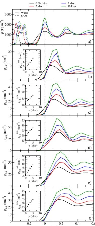
Now we will apply the same methods to the SAM/water interface while also introducing pressure as an additional variable. All ring density proles from four- to eight-membered rings for pressures between 1 bar and 10 kbar are displayed in g. 3.7 along with the mass densities. We observe a much more distinct layer structure in all density proles compared to the vacuum/water interface. The water density oscillates with decreasing amplitude for increasing distance from the interface. The ring densities show the same structure, except the maxima are shifted such that they lie in between the mass density maxima.

This tells us that there is a trivial component to the ring densities caused by an increase in overall water density. If the local water density is higher, the total number of H-bonds increases even if the number of H-bonds per water stays constant (as shown previously in g. 3.4). What we observe here are rings in the H-bond network forming randomly with a higher probability simply due to the high concentration of H-bonds in the density maxima.

Therefore, the probability of nding a ring with its center of mass between the two water density maxima is increased. From this we can infer that there is a preference of rings to align perpendicularly to the interface, because this is the direction in which the water density is structured. This nding is qualitatively true for all ring sizes that we analyzed.

Additionally, the ring density increases continuously with pressure at the interface as well

as in bulk (see insets in g. 3.7), which is also an expected result considering the previous

argument. It is dicult to quantify how the probability of forming rings increases with

density, and neither the relative nor the absolute ring densities change monotonously with

the ring size. Most of the rings in the high density regions are still at least

Å away

from the interface. Next, we focus the discussion on the ring twist

at the low-density

interfacial region. Figure 3.8 contains the twist distributions of four

Å layers starting

at approximately

nm, and the bulk phase for varying pressures. The narrow

distributions of the four-ring twists are almost identical to the twists at the vacuum/water

interface and barely change with the distance from the interface. For ve- and six-rings,

the twists are signicantly lower at the interface than in the bulk. The same eect is still

present but very minor for seven- and eight-rings. By comparing the distributions over

the pressure range up to 10 kbar, we nd that only ve- and six-rings show a signicant

pressure dependence. The twist of ve-rings decreases from 1 bar to 5 kbar, but increases

again at 10 kbar. Only the six-membered ring twist decreases steadily with pressure. We

conclude that pressure appears to increase the preference for low-twist conformations of

six-rings at the SAM/water interface. The fact that this eect is only observed for six-

rings leads us to compare these rings to those found in ice Ih, which is exclusively made of

six-rings. The goal of the subsequent analysis is to compare the rings at the interface in

liquid water and the rings in a single layer of hexagonal ice.

3.2. Results

Figure 3.7.: Proles of H-bond ring densities for ring sizes from 4 (b) to 8 (f) at the SAM/water interface at pressures between 1 bar and 10 kbar with the bulk ring densities in the inset of each panel. (a) is the mass density prole for reference.

(a) Four-membered rings

(b)Five-membered rings

(c) Six-membered rings

(d) Seven-membered rings

(e) Eight-membered rings

Figure 3.8.: Distributions of the ring twistχ_Rof rings in the water hydrogen bond network. The distance of the layers from the interface increases in steps of0.5Å from approximately z=−0.1nm to z= 0.1nm. From left to right, the pressures are 1 bar, 5 kbar, and 10 kbar.

As a rst step, we determine the density of six-rings from a simulation of an ice Ih crystal

along the c-axis. This axis is chosen because the chair-like six-rings which form layers

in ice (g. 3.9 a) are oriented perpendicularly to the c-axis, and because the rings at the

SAM/water interface have the same orientation with respect to the interface, which enables

a direct comparison of the rings in the two systems. Ice Ih contains a second type of ring,

3.2. Results which is in a boat-conformation (g. 3.9 b) and which connects the layers of chair-like rings . Since the two types of rings are spatially separated along the c-axis, we are able to analyze the properties of a single layer of chair-like rings (g. 3.10). The twist distribution inside this layer of rings is very narrow with

of all rings having a twist below

. From now on we dene all rings with a twist below this threshold to be 'ice-like'. Now we can identify these rings with a locally tetrahedral geometry in liquid water. Fig. 3.11 shows a snapshot of a single ice-like ring at the SAM/water interface. Next, the amount of ice-like rings at the interface can be quantied. Instead of determining the absolute density of ice-like rings, we care about the excess density

of ice-like rings at the interface with respect to the bulk phase:

ρ^ex_R(z) =ρ_R(z) Z χ_c

0

[P(χ_R, z)−P_bulk(χ_R)]

d

(3.7) Here

are the total ring densities,

are the ring twist probability densities, and

is the upper cuto for the twist of ice-like rings.

(a) (b)

Figure 3.9.: Snapshots of six-membered rings in bulk ice Ih at 200 K and 1 bar. a) A ring in chair conformation perpendicular to the c-axis. b) A ring in boat conformation. These rings connect the layers of chair-like rings in ice Ih.

(a) (b)

Figure 3.10.: a) Six-membered ring density prole along the c-axis in bulk hexagonal ice Ih at 200 K and 1 bar. The dotted lines mark a layer of rings in chair conformation b) Ring twist distribution of the layer of chair-like rings in a).