Orbital excitations of transition-metal oxides in optical spectroscopy

(1)

Orbital excitations of

transition-metal oxides in

optical spectroscopy

Inaugural Dissertation

zur

zur Erlangung des Doktorgrades

der mathematisch-naturwissenschaftlichen Fakultät der Universität zu Köln

vorgelegt von

Reinhard R¨ uckamp

aus Bensberg

K¨oln, im M¨arz 2006

(2)

Berichterstatter: Prof. Dr. A. Freimuth Prof. Dr. M. Grüninger Vorsitzender der Prüfungskommission: Prof. Dr. L. Bohatý Tag der mündlichen Prüfung: 20.04.2006

(3)

Das Ganze ist mehr als die Summe der Teile.

Diese Arbeit widme ich meiner Familie

(4)

(5)

Introduction

At first sight one might think that orbital physics does not contribute to our daily life but is restricted to the labs of some physicists. For the novel collective phenomena proposed for the orbital degree of freedom this is certainly true at this stage. However, looking at a bottle of green glass its green color is given to it by iron(III) and iron(II) ions which are diluted in the silicon dioxide of which a colorless, transparent glass consists. Visible light that passes through the glass of the bottle is absorbed by these so called color centers in a characteristic way. Our visual perception of the resulting spectrum gives us the impression of green. One might ask: Fine, but where is orbital physics involved here? Well, it happens on the color centers. The iron(III) and iron(II) ions are present in their ground state. By the absorption of photons of a certain energy (corresponding to light of a certain color) the electronic state of the iron ions is changed to an excited state. The excited state differs from the ground state by the occupation of the 3dorbitals (with excitation energies in the visible spectrum). In a free ion all the states that differ only in the 3dorbital occupation have the same energy, i.e. they are degenerate. For an ion within a crystal this degeneracy is lifted at least partially due to the reduction of the rotational symmetry by the crystalline environment. States of different energy will allow transitions between them. For chromium(III) ions in an Al₂O₃ host lattice (well known as ruby) the absorption spectrum is shown in Fig. 1 [1]. Chromium ions in ruby and the iron ions in green glass are isolated and do not interact with each other. However, new fascinating physics will arise in case of interaction between ions with degenerate or nearly degenerate orbital states. The degeneracy then will be lifted by collective phenomena.

Orbital physics requires an orbital degree of freedom in the sense that there is an electronic shell which is partially filled. One class of compounds where this condition is often fulfilled are transition-metal oxides. But these are famous not only for orbital physics. Transition- metal oxides were placed on top of the agenda of solid-state physicists after the discovery of high-temperature superconductivity in the cuprates in 1986 by Bednorz and M¨uller [2].

From this strong activity followed not only an increase of the superconducting T_c up to 134 K, but also the discovery of many unusual physical properties in other compounds of this class. One of the most prominent is certainly the colossal magneto resistance¹ that has been found in the manganites [3]. In many cases only small changes of parameters like variation of doping concentration induce drastic changes in physical properties which lead to rich phase diagrams. This complex behavior is founded in the electronic structure of the transition-

1Colossal magneto resistance denotes a high sensitivity of the resistance of a crystal on a weak applied magnetic field (the resistance drops e.g. about nine orders of magnitude in La1−xSrxMnO3).

(8)

Figure 1: The absorption spectrum of ruby [1]. One observes strong and broad absorption peaks above 15000 cm⁻¹. The absorption peaks reflect transitions between different orbitals.

In the visible spectrum (12500 cm⁻¹ - 25000 cm⁻¹), ruby is opaque except for the range below 15000 cm⁻¹. This is where the deep red color of ruby comes from.

metal ions. The characteristic feature of transition-metal compounds is that the metal ions exhibit a partially filled 3d shell with strong correlations between the electrons. The spin degree of freedom opens the way to a rich variety of magnetic states.

For such a partially occupied shell, band-structure theory predicts a metallic state. How- ever, it is possible that the system is in fact insulating due to the on-siteCoulomb repulsion between electrons. This phenomenon occurs when the bandwidth (kinetic energy gain) is small compared to the strong Coulomb repulsion U. Hence the electrons do not hop to a neighboring site in order to avoid double occupancy. Such an insulator is called Mott insulator. The most important difference from the usual band insulator is that the internal degrees of freedom, spin and orbital, survive in the Mott insulator. The localized electrons occupy a linear combination of atomic states. Interactions of electrons on adjacent sites are mediated on the one hand by the lattice and on the other hand by (virtual) hopping. An increase of virtual hopping lowers the kinetic energy. Thus neither a fully local nor a fully delocalized description applies. A further complication for understanding the physics arises from the strong interaction of several degrees of freedom. In order to solve this problem one has to take all of them into account on an equal footing. At present it is not possible to do so and this intricate problem is far from being understood [4].

In this field of physical research many different new ground states are proposed. The orbital degrees of freedom and the spin degrees of freedom have a similar structure. This

(9)

leads to predictions for the existence within the orbital sector of nearly every effect that has been found in the spin channel. For instance different types of orbitally ordered states, orbital liquids [34], orbital Peierls [8], and the orbital Kondo effect [12] have been predicted. However, there exists a big difference between the orbital and the spin degree of freedom: spins couple only weakly to the lattice, but 3d orbitals do so much more strongly. Interesting physics and also controversial discussions emerge from the competition of the different interactions.

Orbital order may reduce the dimensionality due to the anisotropy of the electron distribution as e.g. in TiOCl (see chapter 5). An even more striking example is KCuF3. It is nearly cubic but due to orbital ordering the magnetic structure turns out to be quasi-one-dimensional [86]. The two-dimensionality of the high-T_c cuprates – although largely due to their layered structure – is substantially enhanced by the fact that the charge carriers (holes) occupy mostly the x²−y² orbitals. Spectacular superstructures are observed in some spinels with transition metals on the B-sites [39]. Examples are an “octamer” ordering in CuIr₂S₄ [9]

or a “chiral” structural distortion in MgTi2O4 [10]. Other interesting orbital physics arise from frustration of the orbital exchange. A prominent example is LiNiO₂ which is suggested to be a realization of an orbital liquid [11]. It is impossible to list here all the interesting phenomena where orbital physics is involved. But certainly the field of orbital physics is very vivid and rapidly expanding.

The central aim of this thesis was the observation of novel orbital excitations. In the literature, reports of orbital waves have been based on Raman measurements [44, 6, 7].

Optical spectroscopy is a well established tool for the investigation of crystal-field excitations and has become a standard method in chemistry [88]. Therefore it provides an excellent means for the study of novel orbital excitations. In particular, the comparison of infrared and Raman data may offer the possibility to decide on the character of the excitations.

This thesis is organized as follows. The first chapter is devoted to introduce the experimental method of Fourier spectroscopy. It includes the physical foundation of optical properties that are presented in this thesis. The second chapter is about orbital physics. It starts with a short review of conventional crystal-field theory, which is the theoretical approach for local crystal-field excitations. The second part reviews the novel ground states that have been predicted for systems investigated in this thesis. As a third subject the orbital excitations of different ground states are discussed.

In the third chapter results on the orbitally ordered compound LaMnO3(Mn³⁺ t³_2g e¹_g) are presented. The key question in this system addresses the nature of the orbitally ordered state.

A conventional scenario invokes a collective Jahn-Teller effect (electron-phonon coupling) as the driving force of orbital order. On the other hand, superexchange (electron-electron coupling) is also proposed to lead to an orbitally ordered ground state. These two possible origins of orbital order can be seen as limiting cases, since in fact both interactions are present simultaneously. However, on the basis of the orbital-order pattern it is not possible to decide which of them dominates as both scenarios are able to explain the experimentally observed orbital order. The orbital excitations play an important role in this context as they are well distinct for the two cases. For dominating electron-phonon coupling they are local crystal-field excitations. In the scenario of strong electron-electron coupling, new collective elementary excitations are predicted which exhibit a significant band width. In 2001 Saitoh et al. [44] reported the observation of peaks in Raman data which have been interpreted as

(10)

collective orbital excitations. This has motivated us to determine the optical conductivity in order to check this claim.

In the fourth chapter we compare our results on the compounds RTiO₃(R = La, Sm, Y;

with Ti³⁺ t¹_2g e⁰_g) which in the sense of orbital degeneracy are a t2g analogue to LaMnO3. The orbital ground state of LaTiO3 has been discussed controversially in the literature [34, 49, 57, 59, 60]. The observation of a small spin-wave gap and a strongly reduced magnetic moment in this compound seem to contradict each other, since the former suggests a small orbital moment whereas the latter indicates a large orbital moment. Khaliullin has explained these observations by the novel orbital-liquid ground state [34]. In this scenario, the orbital occupancy resists long-range order by fluctuations. On the other hand, the reduction of the magnetic moment has been explained by enhanced charge fluctuations due to the small Mott- Hubbard gap within the more conventional picture of an orbitally ordered ground state [57].

The orbital excitations may also here give a hint which ground state is realized.

In the fifth chapter the results on TiOX (X = Cl, Br) (Ti³⁺ t¹_2g e⁰_g) are presented. The bilayer systems are structurally two-dimensional [138]. However, the magnetic susceptibility behaves like in the case of aS = ¹₂ Heisenberg chain at high temperatures [50]. At low temperatures it starts to deviate from the spin-chain behavior and drops to zero below a critical temperature. This has been attributed to a spin-Peierls transition. The one-dimensionality is induced by the orbital ground state in which the occupied orbitals have large overlap only in one direction [50, 143]. Unexpected in a spin-Peierls scenario is however a second transition that occurs at higher temperatures. Due to e.g. a broad NMR signal between the two transition temperatures this behavior has been assigned to strong orbital fluctuations [122].

This motivated us to search for orbital excitations below the electronic gap. Moreover, we measured the phonon range in order to see in how far the lattice is involved in the transitions.

Finally in chapter 6 the results obtained within this thesis are summarized.

In the appendix additional information and some useful results are given which are not new but hard to find in the literature. In part A the Wigner-Eckhart theorem is introduced in the most straight and clear way that we can imagine. In particular the mathematical apparatus is reduced to a minimum. We have not found such a distinct view on the main proposition of the theorem elsewhere in the literature, although it will probably already exist somewhere. Part B gives a detailed view on the structure of the octahedral group O and its representations. In part C and D we provide useful information on the transformation of d-waves under rotations and on p-dmatrix elements, respectively. These have been obtained within the research project of this thesis and shall be made available to others. In part E the Kramers-Kronig relations are derived with some additional hints for readers not familiar with complex analysis. In part F the cluster-calculation model used within this thesis is described briefly.

(11)

Chapter 1

Optics

Optical properties of matter are near to our own sensory perception. For instance we see that the glass of the window is highly transparent and that a metal spoon is well reflecting (if it is polished). Moreover our eyes are sensitive for colors. We find a golden ring shining yellow, a copper wire red, and a silver server shining white. This tells us immediately that copper is reflecting red light very well but other colors (at higher frequencies) much less. For gold the good reflectivity persists for a wider range in the visible spectrum. Silver however is equally reflecting all components we are able to see to a very proportion. So we are familiar with at least a simple form of optical spectroscopy from our daily live. For more detailed information about a certain material we obviously want to know how its optical properties depend on the frequency (or energy, or wavelength) of the electromagnetic wave, and of course we want to investigate not only the visible part of the spectrum but also below and above it, i.e.

the infrared and the ultraviolet spectral range. For this purpose sophisticated experimental setups have been developed which measured the desired properties with very high accuracy.

We discuss this subject later in this chapter. Now we turn to the question:

What can we learn from the optical spectra obtained by such measurements? The first answer to this question is: excitation energies! From the transmittance and the reflectance one can calculate the amount of light that has been absorbed by the crystal. But light (photons) of a certain energy is absorbed only if there are states of the crystal that are at the same amount of energy above the ground state, so that a resonance between the photon and the excitation mode may occur. Therefore peaks in the absorption spectrum provide information on the energy of excitations that do exist in the compound under investigation. However not all excitations existing in a crystal can actually be excited by light but only the ones that are dipole active, i.e. that carry a dipole moment. Another restriction of optical spectroscopy is that a dispersive mode is only probed atk≈0. This is due to the steep dispersion (ω = _n^c ·k with c the speed of light in vacuum) and hence a small momentum k of the photons at the considered optical frequencies. However this is true only for processes involving the photon and only one quasiparticle. If more than one particle is involved in the absorption processes this can lead to zero total momentum whereas the single contributions are located throughout the entire Brioullin zone. For example in a two phonon process the phonons do not have to have k ≈ 0 but can carry an arbitrary momentum |k| if only the total momentum is zero

(12)

(k1 =−k₂). In such a case an absorption continuum is observed in which the information of k-space is inherent in the line shape. This can lead sometimes to an astonishing amount of information on the dispersion if the line shape can be compared with theoretical predictions [55]. Another important source of information on the crystalline properties is provided by the temperature dependence of the spectrum. Across phase transition not only the structural and thermodynamical properties change but in general also the optical spectrum. Moreover the polarization dependence gives additional information on the orientation of the dipole moments in the crystal. Structural information is obtained from the phonon energies and their polarization dependence.

In conclusion optical spectroscopy provides a powerful tool for investigating the properties of crystals. This holds equally for insulators and metals, as opaqueness is not a general problem but can be overcome by a Kramers-Kronig analysis of the reflectance spectrum, which is discussed in Appendix E.

1.1 Interaction of light with matter

In this section we will discuss the description of the interaction of light and matter. First we will consider the description on a macroscopic level, and turn than to the microscopic view as a second point. There we will consider the Drude-Lorentz model in detail. This model explains the shape of the quantities observed in experiment. However, preluding the discussion of the optical properties we will introduce the more general concept of response functions to which for instance the optical conductivity and the electrical susceptibility belong.

1.1.1 Response function

Every experimental result we may obtain of a certain crystal has the form of an answer of the crystal to an applied perturbation. For instance we apply a voltage and measure the responding current or we apply a magnetic field and measure the magnetization and so on. A compact form to describe the interaction of a system with an external perturbation p is provided by a response function G. This function gives the connection between the perturbation p(r, t) as function of spatial position r and time t and the response a(r, t)of the crystal, which is also a function of r and t. Since the response may be delayed and at a different place, one has to account for all perturbations in time (only before the response) and space. This is a rather complex connection between the stimulus and the response. It can be simplified by the assumption of a linear relation of the response to the amplitude of the stimulus.¹ Assuming linearity we are able to write down the following:

a(r, t) = Z

G(r,r⁰, t, t⁰)p(r⁰, t⁰)d(r⁰, t⁰)

This general connection of the perturbationp and the responsea(answer) can be simplified for our case of the interaction of light and matter in several ways (we will also assume a weak field for which we are in the linear regime).

1The assumption of linearity is reasonable if the perturbation added to the Hamiltonian is small. The amplitude is not that large that higher orders contribute.

(13)

• The spatial dependence of the response functionGis suppressed, i.e. we do not account for a perturbation elsewhere in the crystal. This is justifiable since the transport of the perturbation through the crystal by quasiparticles like for instance phonons is rather weak compared to the original perturbation. This definitely changes in the regime of non-linear optics.

• The time dependence takes into account only the time difference between the perturbation and the response. SoGis a function of (t⁰−t) only.

Altogether the above equation is reduced to:

a(t) = Z

G(t−t⁰)p(t⁰)dt⁰

whereG(t−t⁰) = 0 for timest < t⁰ to obey the principle of causality (no response before the perturbation). The responsea(t) is therefore just the convolution ofG(t−t⁰) andp(t⁰). Such an integral appears as a simple product in Fourier space²:

a(ω) =G(ω)·p(ω)

An example for a response function in Fourier space is the dielectric functionε(q, ω) D(q, ω) =ε(q, ω)E(q, ω) .

Here qdenotes the wave vector. In real space this equation reads D(r, t) =

Z ∞

−∞

Z t

−∞

ε(r,r⁰, t)E(r⁰, t⁰)dt⁰dr⁰ .

This shows that it is convenient to consider the response function in Fourier space.

Finally we discuss the derivative with respect to the time coordinate becomes merely a factor −iω in Fourier space which we will use below:

∂

∂tf(t) = ∂

∂t Z ∞

−∞

e^−iωtf(ω)dω

=

Z ∞

−∞

∂

∂te^−iωtf(ω)dω

=

Z ∞

−∞

e^−iωt(−iωf(ω))dω

⇒ ∂

∂tf(t) −→ −iωf^{F T} (ω) Analogously one obtains for one spatial dimension:

∂

∂xf(x) =iqxf(qx)

2Expanding the two “real-space” functions in series of cosine functions, i.e. Fourier-transforming them, one finds that - due to the orthogonality of the cosine functions (R∞

−∞cos(ωit) cos(ωjt)dt=δi,j) - only terms with equal frequency contribute. The product in the integral is hence merely the simple product of the expansion coefficients for equalω.

(14)

1.1.2 Macroscopic properties

We start with the Maxwell equations in SI units and use this system of units throughout this thesis. We will present here a derivation of quantities describing the optical properties of solids, namely the dielectric function ε(ω) and the optical conductivity σ(ω) as well as an equation connecting both. To take into account that these two functions are generally defined as complex functions, we denote them with a hat wherever there can be confusion:

ˆ

ε=ε₁+iε₂ and ˆσ=σ₁+iσ₂. Our starting point will be the Maxwell equations³: dD = ρ D = ε₀? E dE = −B˙

dB = 0 H = _µ¹

0 ? B dH = j+ ˙D

The charge density ρ and the current density j amount for all charges and all currents.

Even for a crystal in vacuum we will not get rid of these two properties, since any interaction with electromagnetic waves will eventually dissociate the formerly neutralized charges and hence giveρ6= 0 andj 6= 0. It is therefore convenient to divide the total quantitiesρ_total, j_total into two parts. One will apply to the external chargesρ_extand currentsj_extwhich we are able to control and which will be zero in case of a perturbation of the crystal by an electromagnetic wave. The other part accounts for the charge density ρmat and current density jmat which arise within the crystal by the interaction with an electromagnetic wave. This part usually defies control. Because we do not know its microscopic appearance, it will enter the Maxwell equations in a kind of black box. Introducing two auxiliary properties D and H (which do not have a physical meaning) the electrical flux Dand the magnetic fieldH are replaced by

D=D+P H=H−M . Here P is defined by

ρmat=−dP and M by

j_mat−P˙ =dM ,

accounting for the contribution raised within matter. The polarization P and the magnetization M are contributions to D and H, respectively, depending on the electric and the magnetic field applied to the crystal. Like the above Maxwell equations that are containing all charges and currents, the resulting modified Maxwell equations - where we have separated the contribution arising from matter - are exact.

dD = ρ_ext, D = ε₀? E+P(E), dE = −B˙

dB = 0, H = _µ¹

0 ? B−M(B), dH = jext+ ˙D

3We make use of the more concise calculus of differential form [5] instead of the conventional vector analysis.

The major theoretical benefit of this formalism is that it does not require the underlying space to be euclidian but only needs an analytic manifold (something that only locally looks like an euclidian space).

(15)

The problem of the unknown contribution of charges and currents has been shifted to the problem of knowing the functionsP(E) andM(B)⁴. So the discrimination between external and matter-inherent charges and currents does not help in order to get an exact solution for a microscopic description. But it opens the opportunity to include approximations for the contributions of charges and currents within matter.

We will make use of this opportunity and refer to the linear approximation in the following considerations. The response of the system (crystal) ought to be linear in the perturbation.

This means that the polarization P is a linear function⁵ inE, and the magnetization M is linear inB. In space and time coordinates this yields the still cumbersome equations

P(r, t) = ε0

R R χˆel(r, t,r⁰, t⁰)? E(r⁰, t⁰)dr⁰dt⁰ M(r, t) = µ⁻¹₀ R R

ˆ

χmag(r, t,r⁰, t⁰)? B(r⁰, t⁰)dr⁰dt⁰ . The Fourier transformed equations however look much more simple:

P(q, ω) = ε0χˆel(q, ω)? E(q, ω) M(q, ω) = µ⁻¹₀ χˆmag(q, ω)? B(q, ω)

so we will consider Fourier space from now on. The response functions ˆχ_el and ˆχ_mag depend in general not only on the frequency ω but also on the wave vector q. Due to the tiny momentum of photonsq≈0 we will consider onlyq = 0 in the following. Then the so called material equations look like

D(ω) = (1 + ˆχel(ω)) ε0? E(ω) H(ω) = (1−χˆmag(ω)) µ⁻¹₀ ? B(ω).

The dielectric function ˆε is therefore defined as ˆε = 1 + ˆχ_el. It depends on many parameters, for instance temperature or the polarization of the electrical field relative to the crystallographic axes (which makes ˆε in general a tensor of rank 2), but for our purpose only the dependence on the frequency of the electromagnetic wave is of relevance: ˆε= ˆε(ω).

Analog one may define the relative magnetic permeability ˆµ(ω) as ˆµ⁻¹ = 1−χˆ_mag. With this the material equations are of the form

D(ω) = ε₀ε(ω)? E(ω) H(ω) = µ⁻¹₀ µ⁻¹(ω)? B(ω).

4Talking here about functionsP(E) andM(B) is making an implicit requirement on the system we consider.

Namely the system may be considered to be homogenous on a relevant scale set by the wave length of the light. This condition is certainly fulfilled in the case of optical wavelengths of some hundred nm in contrast to the inhomogeneity of crystals which usually is less than 1 nm.

5For anisotropic systems the function turns out to be a tensor of rank 2. Note that in this case 1 +χis interpreted as

0

@1 0 0

0 1 0

0 0 1

1 A+

0

@χ11 χ12 χ13

χ21 χ22 χ23

χ31 χ32 χ33

1 A

(16)

In the following we will derive an equation which relates ˆε(ω) and ˆσ(ω). Since the electrical interaction is usually dominating the magnetic interaction by orders of magnitude and so it is justifiable to neglect the magnetic contribution completely in the following and assume a non-magnetic crystal (χmag= 0, µ(ω) = 1).

An additional consequence of the linear approximation is that Ohms law can be applied.

It states that

jmat(ω) = ˆσ(ω)D(ω) = ˆσ(ω)ε0? E(ω).

Here j_mat denotes the conducting current. The conductivity σ depends also on many parameters but anyway we regard it here as a function of ω, σ = σ(ω). Now we return to jmat−P˙ = dM which is in fact the Ampere-Maxwell law (j−D˙ = dH) restricted to the matter inherent charges.

We refer to the assumption of a nonmagnetic crystal M = 0 (⇒dM = 0) which yields jmat−P˙ = 0 .

The Fourier transform of ˙P(t) is−iωP(ω) (see section 1.1.1). Thus we can rewrite the above equation as follows

σ(ω)ε₀? E(ω) +iωP(ω) = 0 Inserting P(ω) =χ_el(ω)? E(ω) we obtain

σ(ω)ε₀? E(ω) +iω χ_el(ω)? E(ω) = 0 (σ(ω)ε0+iω χel(ω))? E(ω) = 0 .

This must hold independent of the electrical fieldE(ω) and hence we get σ(ω)ε₀+iω χ_el(ω) = 0

which is equivalent by the use of χ_el(ω) =ε(ω)−1 to the common form⁶: i σ(ω)

ω = ε(ω)−1 ε₀ Split up into real and complex part this yields

σ1 = ω ε0

ε2 and σ2 = ω ε0

(1−ε1)

6This equation is often presented in cgs units where it reads:

4πi σ(ω)

ω =ε(ω)−1

(17)

Figure 1.1: Two different mechanisms leading to a dipole moment of an insulating ionic crystal. (a) Shift of the negative electron cloud against the positive nucleus. (b) Shift of negatively charged ions M₂ against the positively charged ions M₁.

1.1.3 Microscopic description

We will describe now the microscopic model for the interaction between an electromagnetic wave and matter, i.e. we will open the black box of the macroscopic view. We start with the classical picture assuming classical oscillators present in the crystal. This model is known as Drude-Lorentz model. Clearly the oscillating electromagnetic field will displace charges from their equilibrium position of the ground state and create thereby an oscillating dipole moment. In the following we will neglect again the presence of the magnetic field simply because the magnetic interaction is rather weak compared to the Coulomb interaction. For an insulating, ionic crystal (the kind of crystals considered in this thesis⁷) the displacement of charges can be separated into different contributions shown in Fig. 1.1.

One way to create a dipole moment is to shift the negatively charged electron cloud against the positively charged nucleus. However, the resonance of this so called electronic polarization is at high frequencies, far above the visible. The second possibility is to displace the negatively charged ions against the positive ones (ionic polarization). Its resonance frequencies lie in the far-infrared region. In other terms this is nothing else than the coupling of the photon to phonons (lattice vibrations). In metals the free charge carriers provide another way to create a dipole moment which is resonant down to zero frequency due to the absence of a force opposed to the displacement. For paraelectric crystals the orientation of already existing electrical dipole moments provides a further mechanism. In a quantum mechanical view in principal a transition to any state higher in energy will contribute if it is dipole allowed.

However, we will treat the more instructive classical case here.

Consider now an electromagnetic wave interacting with an ionic crystal. Here, we will restrict the discussion to the process of ionic polarization. The strength of the interaction depends on the frequencyωof the electromagnetic wave with respect to the eigenfrequencyω₀ of the lattice vibration. This is actually the phenomenon of forced oscillation well known from

7An ionic crystal consists of different charged ions as for example NaCl (Na⁺¹Cl⁻¹), whereas for example pure silicon is not ionic since the ions are all equal and therefore by symmetry they can not be charged differently.

(18)

0.0 0.2 0.4 0.6 0.8

1.00.4 0.8 1.2 1.6 0.8 1.2 1.6

0.0 0.2 0.4 0.6 0.8 1.0

0.4 0.8 1.2 1.6

-40 -20 0 20 40

0.8 1.2 1.6

-40 -20 0 20 40

Refl. d = 0.1 (1/ω

0) Refl. d = ∞

Trans. d = 0.1 (1/ω

0) Trans. without interference

Reflectance / Transmittance

2

γ = 0.01 ω₀

1 ε_∞ = 3.0 ω_p = ω₀

ε1

σ1

Ferquency (ω₀) γ = 0

3

ε1

σ1/3

Ferquency (ω₀)

Figure 1.2: Top panels: typical shape of the transmittance T and the reflectance R for a phonon mode is shown. The data have been generated in two ways: 1) accounting for finite thickness effects (the data exhibits strong interference fringes) 2) neglecting multiple reflections. Bottom panels: Optical properties corresponding to R and T are depicted. The case of zero damping is shown on the left hand. The panels on the right hand display the same data but for a finite (weak) damping.

classical mechanics. Let us discuss the frequency dependence of optical properties like the dielectric function ε(ω) and the optical conductivityσ(ω) as well as of measured properties like the reflectanceRand the transmittanceT. In the left panels of Fig. 1.2, these properties are shown for the case of vanishing damping of the oscillators. For clarity we consider here only one mode of the system at the eigenfrequencyω₀, in real systems there are usually more than one mode. In the bottom left panel the frequency range is divided by dashed lines (at ω0 and ωL) into three parts.

• At frequencies much lower thanω₀ the system is following the oscillating field more or less, so the dielectric function (or the amplitude of the displacement) has values similar

(19)

to the static case (ω = 0). Increasing the frequency of the electromagnetic wave towards ω0, the amplitude of the oscillating dipole moments in the crystal are rising more and more and diverge atω =ω₀. This unphysical behavior follows from the assumption of vanishing dampingγ. The increasing amplitude of the oscillations forω →ω0 leads to an increase of reflectance, i.e. the reflectance approaches 1 for ω → ω0 and therefore the transmittance decreases. The energy inherent in the electromagnetic wave is not transferred to the oscillators forγ = 0 except atω =ω0.

• Above ω₀ one might expect a situation approximately symmetric to that below ω₀. However, this is by no means the case. This asymmetry emerges from the fact that the phase shift θ between the electromagnetic wave and the oscillations of the dipoles within the crystal jumps from 0 forω < ω₀ to π/2 at ω₀ and finally to π for ω > ω₀. This discontinuity at ω₀ results again from the non-physical assumption of vanishing dampingγ. However, for weak damping things do not look much different from the case of completely vanishing damping. A phase shift ofπmeans that the dipole moments are oriented just opposite to the applied electrical field, i.e.ε(ω) becomes negative for ω >

ω0. The electromagnetic wave and the outgoing wave of the oscillators are compensating each other in the crystal. The electromagnetic wave is therefore completely reflected and the transmittance is zero. If ω is moving further away fromω₀, the dielectric function stays below zero as long as the dipole oscillation can compensate the electromagnetic wave. For increasing difference ω−ω₀ this mechanism is getting less efficient. The amplitude of the oscillators is decreasing which means that the penetration depth of the light is increasing.

• The dielectric functionε₁(ω) will reach zero at a frequencyω_Lcalled plasma frequency.

The dielectric function approaches ε1 = 1 for ω → ∞. For a single oscillator, there thus has to be a zero of ε1 between ω0 and ∞. Additional oscillators are assumed to be far away and can be included by a constant offset of ε₁ which is denoted ε∞. The frequency ωL is the eigenfrequency of a longitudinal oscillation. The difference between the transversal and the longitudinal mode is shown in Fig. 1.3. To avoid any misunderstanding, the longitudinal mode is never excited by a transversal wave. The longitudinal mode has nothing to do with the absorption process, it is just giving the frequency of vanishingε1 its name. For frequencies aboveωLthe transmittance is rising and the reflectance is decreasing.

From the formal functional form of ε(ωL) depending onε(0), ε∞ and ωT

ε(ω_L) =ε∞+ [ε(0)−ε∞] ω₀² ω₀²−ω²

one can deduce the Lyddane-Sachs-Teller relation from ε(ω_L) = 0. This equation relates the oscillator strength with the ratio ofω_L/ω₀.

In the above consideration we have excluded dispersion, i.e. the momentum of the excitations. This is justifiable by the steep dispersion of light which stays in the vicinity of k= 0 for optical frequencies. In a quantum-mechanical picture (the most appropriate) we would

(20)

-- -- -- -- -- -- --

+ + + + + + + + + + + + + + +

- - - -

+ + + + + + + + + + + + + + +

- - - -

+ + + + + + + + + + + + + + +

-- -- -- -- -- -- --

+ + + + + + + + + + + + + + +

- - - -

+ + + + + + + + + + + + + + +

λ λ

+

+ +

- - -

- -

z x

P G

Figure 1.3: The charge distribution of a longitudinal wave on the left is compared with a transversal wave on the right. Both waves propagate in z direction with the same wavelength λ. The black lines indicate planes (perpendicular to z) of vanishing displacement of charges, separating layers of the thicknessλ/2. The wavelength is assumed to be much larger than the unit cell of the crystal so that one may think of a homogeneous medium. This assumption is certainly fulfilled for optical wave lengths. The direction of the local dipole moment is shown by the green arrows. The difference between both waveforms is seen from the charge distribution of adjacent layers indicated by the orange frames. In the case of a transversal wave, the charge distribution in the adjacent layers support the formation of the dipole moment of the layer in between whereas for the longitudinal wave the formation is hindered by the electrical field of neighboring layers. This leads to a strong restriction for the eigenfrequency of the longitudinal mode. Since the net charge is zero no charges can be accumulated within the crystal it follows that macroscopical bydD= 0 (no external charges).

From D = ε₀ ? E+P = ε(ω)? E it follows immediately that ε(ω_L) has to be zero as the gradient of electrical field is clearly dE 6= 0. In short this tells us that the electrical field induced by the local displacement of charges has to be compensated by the field raised by the displacements of the rest of the crystal. This leads to a macroscopic dipole moment for the longitudinal wave since charges at the surface are not compensated.

not talk of forced oscillation describing the interaction of light with matter but of interaction of photons and phonons.⁸ These two particles will interact in general and will therefore loose their own identity in favor of a new mixed mode. This new mode is called polariton.

The polariton dispersion as well as the dispersion of the corresponding unperturbed particles (photon and phonon) is shown in Fig. 1.4.

For photonic energies far below the phononic eigenmode the interaction does not matter a lot for photon and phonon since nearly no resonance occurs. This changes drastically

8We will think of phonons in the following but any dipole-active eigenmode of the system would do as well.

(21)

forbidden frequency range

ω

₀

ω

_L

k c/ ω

₀

( ε

_∞

)

^½

ω / ω

0

0 0

1 1

ω = k c/( ε (0))

^½

ω = k c/( ε

_∞

)

^½

Figure 1.4: The photon-phonon or polariton dispersion is shown by the solid black curve (two branches). The dotted lines give the linear photonic dispersion for ω ω₀ and forω ω₀. The slope is determined by the value of the dielectric function far away from the resonance (ω = 0 and ω → ∞). The frequency range between ω0 and ωL indicated by the hatching is forbidden since in this range no eigenmode exists within the crystal.

around the resonance where the two modes are not distinguishable anymore. The branch of the former photon dispersion becomes the phonon branch and vice versa. So the resonance between the photon and the phonon can be seen as a kind of level repulsion avoiding the crossing of the two branches and hence the corresponding degeneracy.

The above statements were made only for the case of an ionic crystal. However, for metals the above considerations can be applied to the free charge carriers by assigning an eigenfrequency ofω₀= 0 to their oscillations. The electron gas (plasma) is playing the role of the negative ions. The corresponding longitudinal eigenfrequencyω_Lof such an excitation is called plasma frequency. For this longitudinal oscillation of the electron gas within the crystal the corresponding quasiparticle is termed plasmon. Plasmons are not excited by transversal electromagnetic waves (in analogy to the polaritons) but can be observed by for instance inelastic electron energy loss spectroscopy (EELS).

1.2 Fourier spectroscopy

The importance of optical properties for understanding the physics of the solid state has motivated the experimentalists to measure them accurately. The dielectric function or the optical conductivity are hard to measure directly, the quantities one is able to observe in

(22)

Reflectance Transmittance

Absorption

T+A+R= 1

sample

Figure 1.5: Light can be reflected, transmitted or absorbed by a sample. The corresponding three quantities reflectance, transmittance, and absorption together equal unity.

experiment are the transmittanceT and the reflectance R.⁹

As T +R +A = 1 with the absorption A, we will get the latter immediately when measuring T and R. From these two properties we will be able to calculate other optical property. In order to obtain the transmittance (reflectance) of the sample, it is necessary to compare the transmitted (reflected) amount of light with the amount that has hit the sample from the light source. So one always depends on a reference measurement to determine the proportion of transmittance (reflectance) as the quotient of the transmitted (reflected) light to the incoming intensity.¹⁰ The actual setup of switching between the reference and the sample is shown in Fig. 1.6

A straightforward experimental setup for measuring T and R is shown in Fig. 1.7. Light coming from a source with a continuous spectrum is split up into its frequency components by a grid. A narrow frequency range is picked up by a slit, passes the sample and is measured by a detector. Repeating the measurement without the sample, one gets the amount of light of the particular frequency region in the spectrum of the source. The quotient of the intensity that got through the sample and the incident intensity is the transmittance at that frequency.

This method has been used for decades. However, due to some disadvantages compared to a Fourier spectrometer it is more or less replaced by Fourier spectroscopy, especially in the infrared range.

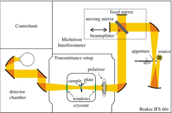
The principle experimental setup of a Fourier spectrometer is shown in Figs. 1.8 and 1.9. The light passes through a Michelson interferometer before hitting the sample. The striking difference to the conventional setup is the absence of a monochromator. So there is no discrimination of the frequency before hitting the sample. Also the detector is not

9In sophisticated experiments also other quantities are observed, e.g. by ellipsometry the ratioRp/Rs (Rp

reflectance of light polarized parallel to the plane of incidence,Rsreflectance of light polarized perpendicular to the plane of incidence) and the phase shiftθ of the reflected light are measured. From these two quantities other optical properties are obtained.

10This is not the case for ellipsometry where no additional reference measurement is needed. Only for calibrating the system a reference sample with known optical properties has to be measured.

(23)

source polarizer

detector hole

sample

source detector

polarizer sample

mirror (gold)

Figure 1.6: The position of the sample and of the reference can be switched rapidly at any temperature. Both are mounted on the same copper plate. The picture is taken from [56].

sensitive to the wavelength of the incident light (in contrast to the human eye). It measures only intensities, i.e. the absorbed energy regardless of the single photon energies. Actually the discrimination between the different frequencies is done after the measurement. The trick is that during a measurement one of the mirrors of the interferometer is moving. Hence the length of the path for the bundle of light reflected at the moving mirror is varying in comparison to the one coming from the fixed mirror. By this the intensity of light of one wavelength is oscillating between constructive and destructive interference with a period that is determined by the mirror velocity and the wavelength. As the velocity of the mirror is the same for all wavelengths, the period of the oscillations is characteristic for the wavelength of the light. The intensity oscillations can be detected by a detector. For a constant mirror velocity the resulting intensity for light of one single wavelength will be a cosine measured as function of the mirror position.

In one scan of the mirror all wavelengths from the source are measured simultaneously,

sample

slit grid

D

Figure 1.7: The principle setup of a spectrometer using a monochromator. The light from the source is passing a grid first. Under a certain diffraction angle, a narrow frequency band with its maximum at that angle is selected by a slit. The beam is passing the sample and is detected by a detectorD.

(24)

moving

sample

D

l + x l

mirror

Figure 1.8: The principle components of a Fourier spectrometer. On the time scale relevant for the detector, the light from the source has constant amplitude, indicated by the orange line. After passing the interferometer, the amplitude depends on the differencex(relative to the wavelength) of the paths the two beams have traveled before interfering. Upon moving one of the mirrors, the amplitude oscillates in time between constructive and destructive interference as indicated by the oscillating orange line. After passing the sample the intensity is measured by a detectorD.

giving a superposition of all cosine terms from all frequencies contained in the spectrum of the source. The intensity as a function of the position of the mirror is called interferogram.

An example of an interferogram is given in Fig. 1.10. The original spectrum is obtained by decomposing the interferogram into cosine terms. The coefficient obtained for one frequency indicates the amount of light with the corresponding frequency contributing to the spectrum.

This decomposition is actually a Fourier transformation, from which the name of the method is derived from.

So far we have discussed the basic mode of operation of a Fourier spectrometer. However, there are more components which are essential for receiving the spectrum of the sample. First it is important to determine the way the mirror moves in order to find the correspondence between the frequency of the cosine terms and the actual wavelength of the light. This is done by measuring additionally the interferogram of a laser which is detected by a diode after passing the interferometer. The laser gives a well-defined cosine signal. Since the laser intensity is orders of magnitude stronger than the intensity of the light coming from the source, the signal obtained by the diode is not influenced by the light of the source. The signal detected by the diode is used to trigger the detector, so that a data point is collected whenever the mirror has moved by one laser wavelength.¹¹ The laser wavelength is known with high accuracy of 1 to 10⁶. Compared to the use of a momochromator, the advantages

11In between two minima of the diode signal the detector is triggered electronically, giving a higher density of data points. This is needed to measure a broader range of frequencies. With the density of data points acquired for a laser frequencyωL, only a frequency interval of widthωL/2 can be measured.

(25)

beweglicher Spiegel

fester Spiegel

Michelson Interferometer

Lampe Blendenrad

Fokus Probenkammer

(bei Transmission) Kontrollelekronik

Detektorkammer Detektor

Strahlteiler

Kryostat Fenster Probe Blende fl. N₂

Polarisator

Bruker IFS 66v detector

chamber Controlunit

sample

windows

polarizer

apperture source beamsplitter

fixed mirror moving mirror

cryostat Michelson Interferometer Transmittance setup

Bruker IFS 66v plate

Figure 1.9: Sketch of the Bruker IFS 66 v/S. All results within this work were obtained with this spectrometer.

of Fourier spectroscopy in the infrared range are

• short measuring times due to the measurement of all frequencies simultaneously.

• the resolution depends only on the length of the interferogram. It can be increased by increasing the distance the mirror moves. Therefore no intensity of the signal is lost, i.e. the signal-to-noise ratio is independent of the resolution.

• due to the precise knowledge of the laser wavelength, Fourier spectroscopy has a very high accuracy in frequency.

• for the short measuring times all other parameters like for instance the temperature stay constant between measuring the sample and the reference.

Triggered by the laser interferogram, the spectrum consists of discrete data points. There- fore a discrete form of the Fourier transformation has to be used.

S(k· 4ν) =

N−1

X

m=0

I(m· 4x) exp(i2πkm/N) In comparison with the continuous transformation

(26)

S(ν) = Z

I(x)·exp(i2πν)dx

one finds a one-to-one correspondence by k·∆ν≡ν,m·∆x≡x, and regarding that the sum runs only over a finite range due to the finiteness of the interferogram.¹² Performing the Fourier transformation one has to be careful since only the measured interferogram has unambiguous physical relevance. The resulting spectrum depends on some choices one has to make when applying the Fourier transformation. This ambiguity is due to the finite length of the interferogram, whereas the cosine function extends from −∞ to∞. The finite interferogram may therefore be regarded as an infinite interferogram times a function (apodisation function) that is identical 0 beyond the range of the measured interferogram. The Fourier transformation is also sensitive to this function, i.e. the result of the Fourier transformation is a convolution of the infinite interferogram (which would give the unaltered spectrum) and the apodisation function. However, this effect gets important only for rapid variation of the intensity within the spectrum, i.e. for very sharp lines (compared to the frequency resolution).

Such features occur in spectra of for instance molecules. About the results presented in this work we do not have to worry.

Another point one has to keep in mind when applying the Fourier transformation is that the frequency range under investigation is at least as wide as the physical spectrum of the light source. Otherwise frequencies higher than the cut-off frequency are folded back, falsifying the resulting spectrum. It is also worth to note that the resolution of thespectrumcorresponds to the length of the interferogram, and that the resolution of the interferogramdetermines the width of the spectral range obtained. This correspondence opens the opportunity to increase the density of points in the spectrum by adding zeros to the interferogram. However, this is not increasing the information but corresponds to a spline through the discrete spectrum. The final remark is about the occurrence of a phase6= 0 of the cosine terms due to a deviation of the mirror symmetry of the measured interferogram at the white-light position. The asymmetry results form the discrete structure that is in general not centered exactly at the white-light position. This phase shift is corrected by taking the absolute value of the amplitude.

In conclusion, Fourier spectroscopy is an excellent tool for the investigation of optical properties of matter. It is fast and provides a very high accuracy. The commercially available spectrometer comes along with a software which makes the measuring procedure rather convenient and the results very satisfying.

1.3 Sample preparation

The method of optical spectroscopy needs planar surfaces of the crystals under investigation in order to give exact values for the measured (and the related) properties. Scattering at surface defects for instance will lead to an overestimation of the absorption. In the transmittance,

12Also common is the form where ω = 2πν is used instead of ν. This gives an extra factor of 1/2π from the substitution dω = 2πdν. This factor is split up by the convention in order to restore the symmetry between the two directions of the transformation: S(ω) = 1/√

2πR

I(x)·exp(i ωx)dx and I(x) = 1/√

2πR

S(ω)·exp(−i ωx)dω.

(27)

Figure 1.10: In the upper panel an interferogram is shown. The peaks (white-light position) correspond to the position for which both mirrors have equal distance to the beamsplitter.

Two peaks occur because the mirror has been moved forward and backward, crossing the white-light position twice in one scan. In the lower panel the part between the dashed lines (in the upper panel) is plotted on an enlarged scale in order to show the detailed structure of the interferogram. The inset displays the fine structure of the interferogram away from the white-light peak. It has the same x axis as the whole panel but is enlarged iny direction.

this effect is increasing with decreasing thickness, i.e. decreasing total absorption within the sample. It is therefore important to prepare samples with a high planarity of the surface.

For transmittance measurements it is also important to have two parallel surfaces in order to have a well defined thickness. The standard procedure for preparation of such a sample is grinding and polishing afterwards [55]. This has been done mechanically, using a commercial polishing machine. The results have been checked under a microscope. For a well polished surface there were no defects or surface roughness observed by a magnification of 64 times.

An estimation of the surface roughness is provided by ellipsometry measurements where in modeling the data of LaMnO₃ the parameter for the surface roughness could be determined to be <3 nm [33]. This procedure has been applied to all samples investigated within this work except TiOX which will be discussed later (see chapter 5).

(28)

(29)

Chapter 2

Orbital physics

In this chapter the state of the art of orbital physics is presented. It is divided into three parts. In the first part a summary of the basic ideas of the crystal-field theory is given. This is well established since the 1960’s. The second part treats more recent approaches for novel scenarios of collective orbital physics. In the third part we will discuss how orbital excitations ought to appear in the optical conductivity.

2.1 Local orbital physics

For electrons in a crystal there exist two limiting cases. Weakly bound electrons delocalize completely and can not any longer be assigned to a single site. These electrons are forming bands and they are best described by band-structure calculations. On the other side there are electronic states of core shells which are strongly bound deep in the potential of the nucleus.

These electrons feel the crystalline environment only as a small perturbation which adds to the Hamiltonian of the free ion. Here we will consider the partially filled 3d shell. Band structure theory supposes that a partially filled 3dshell forms a conducting band. However, many transition-metal compounds turn out to be pretty good insulators. The insulating property originates in a comparably small bandwidth and a strong Coulomb repulsion. A double occupancy on one site is several eV higher than the ground state. This prevents the 3d electrons to leave their sites although there were unoccupied states available. This class of insulators is called Mott-Hubbard insulators. It is therefore justifiable to consider the transition-metal ions in a local limit and add the influence of crystalline environment only as an electrostatic potential at the metal site. Effects due to the interaction of adjacent metal sites are apparently neglected within this limit.

The electronic state within the 3dshell of a transition-metal ion in a crystal is characterized by its spin and orbital state. In a partially filled 3dshell the fivefold orbital degeneracy of a free ion is lifted by interaction with the crystal, yielding orbital multiplets of different energy. The most important interaction of the ion with the crystal that accounts for this splitting is the Coulomb potential present at the ion site. It originates from all other ions in the crystal. The other interaction we will take into account is the hybridization with the ligands. The splitting of orbital states gives rise to the possibility of transitions between

(30)

different states. These so-called orbital excitations have been observed in optical spectra for many decades and so far were successfully described by the local approach of crystal-field theory that we will consider in the following in detail. The method of crystal-field theory is also the approach behind the cluster calculation performed within this thesis.

2.1.1 Crystal-field theory

We will restrict ourselves to the case of an open 3d-shell of a transition-metal ion in a crystal.

Let us initially assume a crystal field of octahedral (or cubic) symmetryObecause it provides the predominant part of the crystalline field not only in the compounds investigated in this thesis but also in many other transition-metal oxides. The most simple case that may occur is that of one electron in the 3dshell. In the free ion (no crystal around) the electronic state is fivefold orbitally and twofold spin degenerate due to the full rotational symmetry SO(3).

So there are 5×2 = 10 degenerate states. These states are characterized by the eigenvalues of S and L since these are good quantum numbers (in a first approximation we neglect the spin-orbit coupling). Reducing now the symmetry fromSO(3) toO,Lis no longer a constant of motion and one expects to lift the tenfold degeneracy at least partially. The degeneracy according to the spin will not be lifted except a magnetic field is applied which breaks the time-inversion symmetry.¹ The radial wave function is suppressed in the following since only the angular dependence is affected by the reduction of symmetry. Our task is to find the new eigenstates and the corresponding eigenvalues. The Hamiltonian of the free ion

H0 = ∇²

2m +V(r)

(V(r) accounts for the potential of the nucleus and electrons of the inner shells) is solved by the hydrogen wave functions. The potential aroused by all other ions of the crystal (the crystal field)VCF has to be added toH0,

H =H₀+H_CF .

The crystal field represents only a small perturbation compared to the field of the nucleus and hence perturbation theory can be applied. The eigenfunctions of the unperturbed system are denoted by |ψi. They form a basis of the 10-dimensional Hilbert space of the free ion.

Diagonalization of the matrix (H_ij) =hψ_i|V_CF|ψ_ji yields the eigenvalues and eigenstates of the perturbed system. The new eigenstates are linear combinations of the 10 spin-orbital states. These states have to transform under operations of the octahedral group according to a representation of O. It turns out that the representation ofSO(3) for L= 2 splits into the representations E+T₂. We neglect the spin-orbit coupling here and discuss it later in this section. The degeneracy of the spin state is not affected and will be suppressed in the following. Since the rotational symmetry is nearly lost for a strong crystal-field splitting, the corresponding eigenfunctions are combinations of the angular momentum eigenfunctions to

1For systems with an odd number of electrons there exists always a twofold spin degeneracy which is called Kramers doublet. The origin of this degeneracy lies in the time-inversion symmetry. Putting it in other words, the odd number of spins can not be coupled toS= 0 and hence the spin states of (Sz=±¹₂) have the same energy if no magnetic field is present that breaks time-inversion symmetry.

(31)

free ion

cubic CF E_g

T_2g 10 Dq

Figure 2.1: On the left the lifting of degeneracy by reduction of the symmetry from full rotational to cubic is shown for a 3d¹ configuration. On the right the angular dependence of the basis functions 3z²−r², x²−y² (red,eg symmetry) andyz, zx, xy (blue,t2g symmetry) is displayed.

mL= 0, i.e. standing waves without a complex phase. The angular dependence of the angular momentum eigenfunctions for L= 2 – the spherical harmonics – are denoted by |l m_li.

u = |2 0i = _4r¹2

q5

π 3z²−r² v = ^√¹

2(|2 2i+|2 −2i) = _4r¹2

q15

π x²−y² a = ^√ⁱ

2(|2 1i+|2 −1i) = _2r¹2

q15

π yz

b = ^√¹

2(−|2 1i+|2 −1i) = _2r¹2

q15

π zx

c = ^√ⁱ

2(−|2 2i+|2 −2i) = _2r¹2

q15

π xy

These functions are refered to as{u, v, a, b, c}or{3z²−r², x²−y², yz, zx, xy}, respectively.

The first two belong to the E_g and the other three to the T_2g representation (the subscript g gerade – german for even – indicates the behavior under inversion). The energy of the E_g states are raised by an energy of 10Dq with respect to theT2g states, where the energyDq is given byDq =h2 2|V_CF|2 2i. Hence the parameter 10Dq represents the strength of the cubic crystal field. If the symmetry of the crystal field is lower than cubic, this leads to a further reduction of degeneracy. The results above are visualized in Fig. 2.1.