Real Estate Investments, Regulation, and Financial Intermediation

and Financial Intermediation

Dissertation zur Erlangung des Grades eines Doktors der Wirtschaftswissenschaft

eingereicht an der Fakultät für Wirtschaftswissenschaften der Universität Regensburg.

Vorgelegt von:

Michael Heinrich

Berichterstatter:

Prof. Dr. Tobias Just, Universität Regensburg Prof. Dr. Steen Sebastian, Universität Regensburg

Tag der Disputation:

02. Mai 2018

First of all, I am deeply grateful for the guidance, advice and support from my rst supervisor Prof. Dr. Tobias Just. I am also indebted to my second supervisor Prof.

Dr. Steen Sebastian for his support and advices. Moreover, I would like to thank Nils-Leif Moser, Dr. Binh Nguyen Thanh, Sebastian Schnejdar, Prof. Dr. Thomas Schreck and Simon Wiersma. Finally, I am grateful to my family for their support.

i

Contents

Acknowledgements i

1 Introduction 1

2 The Impact of Risk-Based Regulation on European Insurers' In-

vestment Strategy 7

2.1 Introduction . . . . 8

2.2 The Solvency II Standard Formula . . . 11

2.3 Data and Calibration . . . 15

2.3.1 Data . . . 15

2.3.2 Calibration of the Solvency II Standard Formula . . . 16

2.3.3 Descriptive Statistics . . . 18

2.4 Portfolio Optimization . . . 20

2.4.1 Attainability of Target Returns and Portfolio Eciency . . . . 20

2.4.2 Eects on the Allocations of Individual Asset Classes . . . 26

2.5 Conclusion . . . 29

2.6 Appendix 1 . . . 31

iii

3 The Determinants of Real Estate Fund Closures 33

3.1 Introduction . . . 34

3.2 The German Open-End Fund Crisis . . . 35

3.3 Related Literature and Hypotheses . . . 37

3.3.1 Fund Run Risk . . . 39

3.3.2 Economies of Scale and Scope . . . 40

3.3.3 Industrywide Spillover Eects . . . 42

3.3.4 Institutional Investors . . . 43

3.3.5 Control Variables . . . 43

3.4 Data, Methodology, and Sample Description . . . 45

3.4.1 Data . . . 45

3.4.2 Research Design and Variable Denitions . . . 46

3.4.3 Descriptive Statistics . . . 49

3.5 Results . . . 54

3.6 Conclusion . . . 70

4 The Discount to NAV of Distressed Real Estate Funds 71 4.1 Introduction . . . 72

4.2 The German Open-End Fund Crisis and Regulatory Background . . . 77

4.3 Related Literature and Hypotheses . . . 79

4.3.1 Financial Leverage . . . 82

4.3.2 Conicts of Interest . . . 83

4.3.4 Spillover Eects . . . 85

4.3.5 Sentiment . . . 86

4.4 Data, Methodology and Sample Description . . . 87

4.4.1 Data . . . 87

4.4.2 Research Design and Denition of Variables . . . 88

4.4.3 Descriptive Statistics . . . 93

4.5 Results . . . 97

4.6 Conclusion . . . 104

5 Conclusion 105

Bibliography 108

v

List of Tables

2.1 Descriptive Statistics and Solvency II Standard Formula Calibration . 19

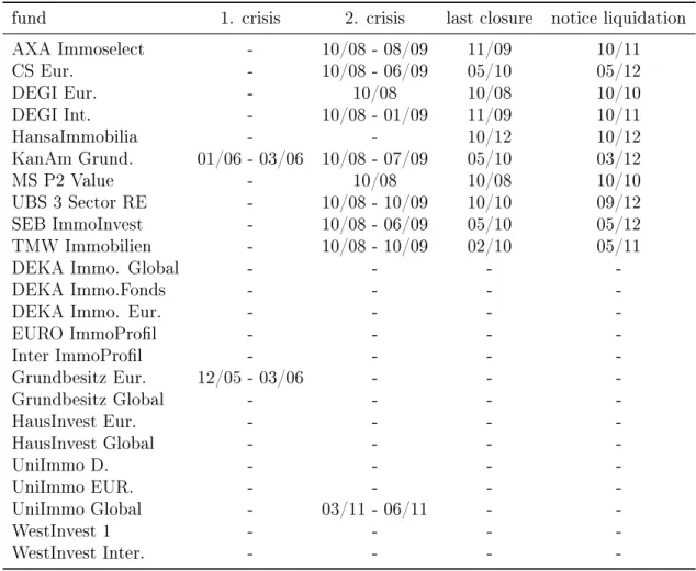
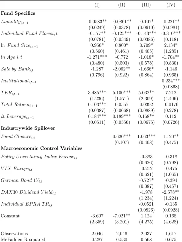
3.1 Overview Open-End Fund Closures and Liquidations . . . 38 3.2 Overview Summary Statistics . . . 49 3.3 Explaining Fund Closure Probability . . . 55 3.4 Correlation Matrix: Fund Specics, Spillover, and Macroeconomic

Variables . . . 61

4.1 Overview of Distressed Open-End Real Estate Funds . . . 79 4.2 Overview Summary Statistics . . . 95 4.3 Correlation Matrix: Fund-Specics, External Variables, and Control

Variables . . . 98 4.4 Explaining the Discount to NAV . . . 100

vii

List of Figures

2.1 Optimized Portfolios in the µ -SCR-Space . . . 23 2.2 Optimized Portfolios in the µ - σ -Space . . . 25 2.3 Optimal Portfolio Allocations for Dierent Levels of Basic Own Funds 28 2.4 Optimal Portfolio Allocations . . . 31

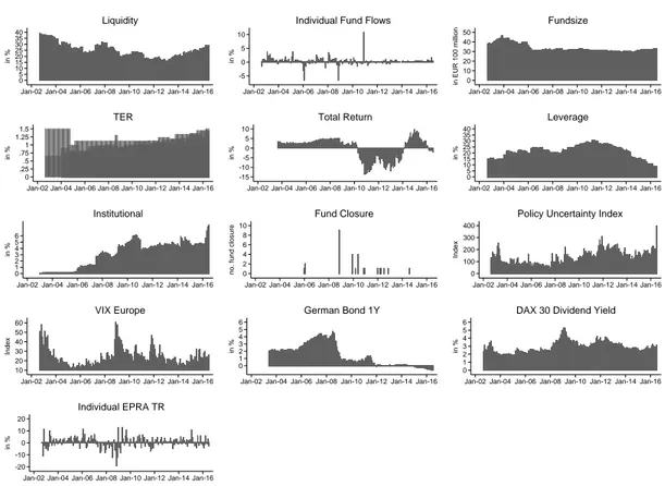
3.1 Overview Open-End Fund Crises . . . 37 3.2 Summary Statistics . . . 50 3.3 Eects of the Liquidity Ratio on the Fund Closure Probability . . . . 56 3.4 Eects of Individual Fund Flows on Fund Closure Probability . . . . 58 3.5 Eects of Fund Age on Fund Closure Probability . . . 59 3.6 Eects of the Sale by Bank Variable on Fund Closure Probability . . 60 3.7 Eects of Fund Size on Fund Closure Probability . . . 62 3.8 Eects of the Number of Fund Closures on Fund Closure Probability 63 3.9 Eects of the Share of Institutional Investors on Fund Closure Prob-

ability . . . 64 3.10 The Predicted Fund Closure Probability of Distressed Funds I . . . . 66

ix

3.12 The Predicted Fund Closure Probability of the Remaining Healthy

Funds I . . . 68

3.13 The Predicted Fund Closure Probability of the Remaining Healthy Funds II . . . 69

4.1 Total NAV Volume and Total Market Capitalization . . . 74

4.2 Discount to NAV . . . 75

4.3 Overview Open-End Fund Crisis . . . 80

4.4 Discount to NAV, Fund Specics, External and Control Variables . . 94

4.5 Development of Time Dummies . . . 103

x

Chapter 1 Introduction

1

Real estate as an asset class can deliver high risk-adjusted returns, which are also low-correlated to the returns of other asset classes, such as stocks and bonds. Ac- cording to the literature, a well-diversied mixed-asset portfolio should therefore comprise between 10% and 30% of real estate.

This holds true for large and medium-sized institutional investors, but also for small retail investors (private in- vestors). However, direct real estate proves to be an unsuitable investment for the vast majority of private investors. The reasons for this include high transaction costs and long transaction periods (leading to low liquidity), the heterogeneity of the assets themselves and the absence of an ecient marketplace (resulting in high due diligence costs) and, above all, the large lot sizes of the individual assets.

The large lot sizes and the indivisibility of direct real estate make it impossible for small investors to create a well-diversied portfolio, consisting of a variety of dierent real estate assets. Even one single direct investment typically exceeds the above- mentioned optimal portfolio weight of 10% to 30% for the vast majority of private investors, leaving them with an unbalanced portfolio containing lump risks.

Fur- thermore, a direct investment would leave the unspecialized private investor with rather high due diligence costs. To sum up, direct real estate involves risks that are not compensated with a risk premium, since they can be diversied and mitigated by increasing portfolio size.

In order to nevertheless prot from the favorable risk-return prole and the diver- sication benets of real estate, private investors can invest indirectly. By doing so, the investor acquires claims against a nancial intermediary (usually in form of fund shares, certicates or policies). The nancial intermediary for its part invests in direct physical real estate.

Due to its portfolio size, the nancial intermediary is able to invest in a large di-

1

Studies examining the optimal real estate quota include Ziobrowski and Ziobrowski (1997), Chun et al. (2000), Brounen and Eichholtz (2003), Hoesli et al. (2004), Bond et al. (2006), Lee and Stevenson (2006), Hoesli and Lizieri (2007), Brounen et al. (2010) and Rehring (2012).

2

For a more comprehensive overview of the shortfalls of direct real estate as an asset class, see, for example, Sebastian et al. (2012).

3

According to the literature, at least 20 to 50 dierent assets are required to diversify most of

the idiosyncratic asset specic risk, see, for example, Brown and Matysiak (2000).

versied real estate portfolio on the one hand, but to issue very small shares on the other hand, thus transforming the lot size substantially.

Furthermore, the inter- mediary is able to transform risk, return and liquidity. Open-end real estate funds in Germany, for example, issue and redeem shares on a daily basis, whereas trading the actual underlying real estate assets usually takes several months. Moreover, the funds issue and redeem shares at the valuation-based net asset value of the underlying properties, instead of at their more volatile market transaction price.

Another example of the transformation of risk, return and liquidity are life insurance policies, also known as life endowment policies. As a private retirement scheme, life insurance policies are illiquid and have a term to maturity of usually more than 20 years. In return, the policies oer a guaranteed minimum return rate, independent of the more volatile and uncertain returns of the underlying assets (i.e. bonds, stocks and real estate).

Both of the aforementioned types of nancial intermediation are popular amongst private investors in Germany. According to GDV (2006), the market for life insur- ance policies has a volume of more than EUR 1.000 billion in Germany alone. With an invested capital of EUR 145 billion, the German open-end real estate fund indus- try is the predominant indirect German real estate investment vehicle and the largest market for open-end real estate funds worldwide.

One reason for the tendency to- wards non-listed indirect investments in Germany can be seen in the widely-held aversion to market volatility and stock ownership amongst German retail investors.

However, nancial intermediaries cannot eliminate but only transform illiquidity and market volatility. Therefore, nancial intermediaries are usually exposed to struc- tural risks in exchange for delivering more stable returns and/or increased liquidity.

4

According to BVI (2017), the portfolio volume of German open-end real estate funds average out at more than EUR 150 million. The share prices usually range from EUR 50 to EUR 100.

5

See Barkham and Geltner (1994) for an examination of the dynamic of prices and valuations.

6

See Downs et al. (2016).

7

According to the 2016 shareholding statistics of Deutsches Aktieninstitut (DAI), the number

of shareholders and investors in equity funds in Germany amounted to only 9 million in 2016. This

equals 14 percent of the German population over the age of 14 years.

Since direct real estate assets cannot be traded on a daily basis, an open-end real estate fund can become insolvent if the volume of its redeemed shares exceeds the sum of its newly issued shares and its cash reserve at any point in time. In this case the fund must immediately suspend the redemption of its shares and may eventu- ally even be forced to liquidate its portfolio, both of which are very unpleasant for the funds investors.

A life insurance company faces insolvency if the guaranteed rates sustainably exceed the return of its portfolios assets. Anticipating this might cause life insurance companies to rethink their asset allocations and shift portfolio weights away from government bonds towards higher yielding asset classes, such as real estate. This in turn may lead to more portfolio risk and regulatory intervention.

This dissertation analyzes the structural risks of open-end real estate funds in Ger- many and of life insurance companies in Europe. Both intermediaries have been exposed to economic uncertainty, low interest rates and regulatory intervention in the aftermath of the great nancial crisis in 2007/2008.

Chapter 2 examines the impact of a new risk-based regulatory framework (Solvency II) on the attainability of target returns, the attainability of portfolio eciency and the asset allocation of European life endowment insurers. The chapter starts with a brief introduction to the Solvency II Directive, focusing on the rules for calculating solvency capital requirements (SCR) according to the Solvency II standard formula.

The subsequent numerical analysis includes several portfolio optimizations focusing on six relevant asset classes for the 1993 to 2017 time period. Optimal portfolios with respect to the Solvency II capital requirements, with respect to conventional risk measures, and a combination of both optimization problems were derived. The results show that the capital requirements according to Solvency II are not ade- quately calibrated. Nevertheless, due to a solid equity base, the majority of Euro- pean insurers are still able to attain high target returns and mean-variance-eciency.

However, undercapitalized insurers are not able to hold risk-optimal allocations of

8

Chapter 4.2 provides some regulatory background on the liquidation regime of German open-

end real estate funds and an overview of the recent crisis.

equities, real estate and hedge funds any longer. In an environment of very low interest rates, these insurers may also face diculties obtaining their target returns.

This is the rst study to explicitly incorporate the solvency capital requirement as a numerical constraint into the insurers' portfolio optimization problem. As a result, the approach shown in this chapter rst provides insights into the attainable target return and the asset weights as a direct function of insurers' equity.

Chapter 3 examines the factors that cause the closing (i.e. the redemption of shares) of open-end real estate funds. During the October 2008 fund crisis, approximately one-third of German open-end real estate retail funds, with total assets under man- agement of about EUR 30 billion, were forced to suspend the redemption of their shares. A fund closure generally leads to fund liquidation, which is a severe issue for management and investors. Subsequent to a closure, the fund management is forced to liquidate the fund by selling the real estate assets. The liquidation often occurs under high selling pressure, and may involve signicant fees. Moreover, in the event of a fund closure, the fund investors' capital is totally constrained. Investors can no longer redeem their shares but only sell them on the secondary market, often at signicantly discounted prices. Thus, knowing the determinants of fund closures could help the fund management to adjust investment strategies and diminish the closure risk. The monthly panel dataset contains fund-specic information such as the liquidity ratio, capital net inows, leverage ratios and management fees for the entire population of German open-end real estate retail funds over the August 2002 to June 2016 time period. The results of the logit model suggest a signicantly positive inuence of fund run risk and industry-wide spillover eects on fund closure probability. The results also indicate that a greater share of institutional investors tends to increase the probability of fund closure. On the other hand, economies of scale and scope decreased the probability of fund closures.

Chapter 4 examines the discount to net asset value (NAV) of closed open-end real

estate funds in Germany. During the global nancial crisis, the German open-end

real estate fund industry experienced massive share redemptions. A total of ten

retail funds with cumulative assets under management of over EUR 30 billion, were forced to suspend share redemptions, and nine funds ultimately liquidated their entire portfolios. Investors of these funds could await the stepwise liquidation of the funds' assets (which usually takes several years) or they could sell their shares on the secondary market, often at a notable discount to net asset value (NAV). This chapter analyzes the discount to NAV of distressed German open-end real estate funds. The hand-collected dataset covers the entire crisis and post-crisis period from October 2008 to June 2016. The analysis shows that the discount to NAV is driven by fundamental risks: It is positively correlated with the fund's leverage ratio and decreases with the share of liquid assets. Moreover, the NAV discounts are related to potential conicts of interest between investors and fund management (TER and extraordinary payouts). The ndings also include that NAV discounts are driven by spillover eects from the announcement of other fund liquidations, as well as by investor sentiment, which is approximated by the aggregate level of capital inows into the industry and by the degree of macroeconomic uncertainty.

The dissertation ends with a conclusion in Chapter 5.

Chapter 2

The Impact of Risk-Based

Regulation on European Insurers' Investment Strategy

Michael Heinrich, Daniel Wurstbauer

7

2.1 Introduction

Short-term and long-term interest rates are currently close to their historical lows, as are yields on top-rated government bonds. For example, the annual yield on new issue 10-year German government bonds was just 0.467% in July 2017, with no sustainable interest rate turnaround foreseeable anytime soon. According to a recent publication by the European Central Bank (ECB), more than half the investments of insurance companies in Europe are in xed-interest securities. Hence, this politically motivated low-interest phase poses a major challenge to the largest institutional investors in Europe, which together hold almost EUR 7.8 trillion of assets.

More precisely, the combination of low bond yields and high interest rate guarantees on existing life insurance policies can result in severe undercoverage for insurers.

The pressure on insurance companies to take action is growing even stronger because the high yielding bonds from the pre-low-interest phase that insurers still hold in their portfolios will mature sooner than the high rate insurance policies. Insurers will therefore be forced to move their investments out of top-rated government bonds into asset classes oering higher returns, such as corporate bonds, equities or alternative investments like real estate or hedge funds.

Several practitioner studies report that European insurers have already expanded their quotas for alternative investments in recent years.

However, the introduction of a new risk-based regulatory framework in 2016 (Solvency II) could have signicant implications on insurers' investment strategy and could even counteract this trend in the months and years ahead. In order to limit their insolvency risk, insurers must now underpin all risky balance sheet items (including investments) pro rata with equity capital. The required amount of equity the solvency capital requirement or SCR varies considerably depending on the respective asset class. From an

1

See ECB (2017).

2

According to an analysis by Assekurata (2016), for example, the average guaranteed interest rate on existing policies among German life insurance companies amounted to 2.97% in 2016.

3

Blackrock (2013), Preqin (2013), Preqin (2015), Insurance Europe and Oliver Wyman (2013),

Towers Watson (2013), EY (2016), EY (2017).

economic perspective, the regulator has introduced a new constraint into the port- folio optimization problem: The aggregate of the SCR for all risk positions must be less than the insurer's amount of equity capital (the basic own funds or BOF). If this constraint is binding, a shift in the portfolio weights is foreseeable. Since the optimized portfolios without the constraint are ecient, the constrained portfolios must exhibit either more risk or less return. Both eects are highly undesirable, considering that the original purpose of the regulation is the mitigation of risk, and that insurers are already facing undercoverage in terms of return.

Most of the existing literature on the eects of Solvency II on insurers' investment policy only deals with specic details of the framework, such as the calibration of the SCR for certain asset classes, for example.

There are, however, two very comprehensive and seminal contributions by Hoering (2013) and Braun et al. (2015), entitled Will Solvency II Market Risk Requirements Bite? The Impact of Solvency II on Insurers' Asset Allocation and Portfolio Optimization Under Solvency II:

Implicit Constraints Imposed by the Market Risk Standard Formula, respectively.

Hoering (2013) states that the aforementioned constraint imposed by the Solvency II standard formula's market risk module is not binding for many European insurers.

He notes that the widely-used Standard & Poor's (S&P) rating model requires even more equity capital than Solvency II for most S&P rating classes. He concludes that insurers with a credit rating of BBB or better will most likely not alter their asset allocation after the introduction of Solvency II. However, Hoering is not examining ecient portfolios in an environment of extremely low interest rates, but rather the investment portfolio of a representative European-based life insurer in 2012. Braun et al. (2015), on the other hand, consider the issue of optimizing an insurance company's asset allocation when the rm needs to adhere to the capital requirements of Solvency II in the context of modern portfolio theory. They run a quadratic

4

Besides the eects on portfolio eciency, a reallocation of insurers' assets could lead to funda- mental shifts in demand and pricing for several asset classes, as Fitch Ratings (2011) has already pointed out.

5

See, for example, Braun et al. (2014), Gatzert and Kosub (2013), Gatzert and Martin (2012),

Severinson and Yermo (2012), Fischer and Schlüter (2012), Al-Darwish et al. (2011), Rudschuck

et al. (2010) and Van Bragt et al. (2010).

portfolio optimization program, and subsequently compute the capital charges for the respective portfolios according to Solvency II. They nd that most of the ecient portfolios are not admissible if the insurer's amount of equity capital is limited to the industry average of 12%. In contrast to Hoering, Braun et al. therefore conclude that Solvency II might cause severe asset management biases in the European insurance sector.

This paper lls the gap between the two aforementioned studies: Depending on insurers' equity capital and investment objectives, Solvency II might render certain target returns unattainable, cause portfolio ineciency or lead to no restrictions on insurers' asset allocation at all. To the best of our knowledge, there exists no previous study that has explicitly incorporated the solvency capital requirement as a numerical constraint into the insurers' portfolio optimization problem. As a result, our approach rst provides insights into the attainability of dierent target returns as a direct function of insurers' basic own funds.

Furthermore, we calculate the critical threshold for the basic own funds needed to attain portfolio eciency at the respective target returns. Ultimately, our analysis provides an in-depth look at how the optimal portfolio weights for individual asset classes will respond to a restriction on insurers' equity capital.

The paper is structured as follows. Section 2.2 presents the market risk standard formula of Solvency II. Section 2.3 introduces the dataset used within the portfolio optimization, as well as the specic calibration of the Solvency II standard formula according to the dataset. In Section 2.4, we run dierent portfolio optimization programs with the solvency capital requirement as an explicit constraint, and present the results. Finally, Section 2.5 concludes.

6

Note that the attainability of a certain target return is necessary to fulll the interest rate

guarantees on existing life insurance policies, as already pointed out.

2.2 The Solvency II Standard Formula

Solvency II codies and harmonizes the insurance regulation inside the European Union (EU). Its primary concern is the amount of equity capital that insurance companies must hold to reduce their risk of insolvency. For this purpose, Solvency II introduced risk-based capital requirements across all EU Member States for the rst time. The solvency capital requirement (the SCR) for an individual insurer can be determined either by using a standard formula imposed by the regulator, or by implementing an insurance internal model. The focus of this paper will be on the Solvency II standard formula, which serves as a reference point for any further analysis.

The Solvency II standard formula refers to basic actuarial principles, and it is cali- brated according to historical data. The standard formula consists of separate risk modules (i.e., risk categories), including market risk, counterparty default risk, life underwriting risk, non-life underwriting risk, health underwriting risk and intangi- ble asset risk. Each of these modules consists of further sub-modules (see EIOPA, 2012). In order to determine a company's overall capital requirement, the capi- tal requirements for all risk modules (and sub-modules) are determined rst, and aggregated subsequently by taking into account diversication eects.

The further analysis is focused on the market risk module, which is of particular importance as its capital requirements depend directly on the insurers' asset alloca- tion. In addition, according to the EIOPA Report on the fth Quantitative Impact Study (QIS5) for Solvency II (see EIOPA, 2011), and according to a study by Fitch Ratings (2011), the market risk module plays the predominant role in determining a company's overall SCR.

The market risk module (SCR

) consists of seven sub-modules: interest rate

risk, equity risk, property risk, spread risk, concentration risk, illiquidity risk and

exchange rate risk. In line with previous studies (see Gatzert and Martin, 2012 or

Braun et al., 2015, for example), the further analysis is limited to the most important sub-modules, which are interest rate risk, equity risk, property risk and spread risk.

Generally, the SCR for each sub-module refers to the change in the basic own funds

∆BOF that results due to a shock or stress in the nancial markets, related to the module's risk category (e.g., a real estate crisis, a shift in the term structure of interest rates, etc.). BOF is dened as the dierence between the market values of assets and liabilities. Without loss of generality, BOF is assumed to equal the equity capital position on the insurer's balance sheet. All specications presented next are taken from the Revised Technical Specications for the Solvency II valuation and Solvency Capital Requirements calculations released by EIOPA (2012).

This document denes the Solvency II standard formula.

The interest rate risk sub-module (M kt

) accounts for the fact that both assets and liabilities react to changes in the term structure of interest rates. As the assets' and the liabilities' interest rate sensitivities are typically not perfectly matched, both upward and downward shocks to the yield curve could theoretically have a negative eect on the BOF. Hence, the capital requirement for interest rate risk depends on two possible states,

M kt

= BOF |

(2.1)

M kt

= ∆BOF |

(2.2) where ∆BOF |

and ∆BOF |

are the changes in the market value of assets minus liabilities caused by an upward or downward change in the interest rate, respectively.

The altered interest rate structures for the two stress scenarios (up and down) are derived by multiplying the current interest rate for any given maturity (r

) by predened upward and downward stress factors ( s

and s

), which are specied and tabulated by the regulator (see EIOPA, 2012):

r

= r

∗ (1 + s

) (2.3)

7

The European Insurance and Occupational Pensions Authority (EIOPA) is part of a European

System of Financial Supervisors that comprises three European Supervisory Authorities.

r

= r

∗ 1 + s

(2.4) In any case, the absolute change in the interest rate for a stress scenario must be at least 1 percentage point, according to EIOPA. In practice, the downward stress scenario is of much greater relevance, especially for life insurance companies. This is due to the typically higher duration of insurers' liabilities compared to assets, causing the market values of liabilities to rise more than those of assets in case of a downward interest rate shock. Moreover, the absolute value of liabilities usually exceeds the absolute value of interest rate-sensitive assets. Hence, only a downward shift of the yield curve has a negative impact on the BOF in the vast majority of cases.

The equity risk sub-module refers to volatility in the market value of equities and its impact on the BOF. Generally, EIOPA distinguishes between two types of equities:

The type 1 equities include all equities listed in countries of the EEA or OECD, while the type 2 equities include all those listed in other countries. Moreover, all non-listed equity investments, such as private equity, hedge funds, commodities and other alternative investments, are also considered type 2 equities. The capital requirement for the equity risk sub-module is determined in two steps. First, the individual capital requirement (M kt

) for each type of equities (i) is determined by the predened stress factors:

M kt

= max(∆BOF| equity shock

; 0) (2.5)

The stress factors for type 1 and type 2 equities are 39% and 49%, respectively.

These gures are based on historical total return data, and refer to the value at risk

(VaR) with a condence level of 99.5% on an annual basis. Second, the resulting

overall equity risk SCR is calculated using a preset correlation matrix imposed by

the EIOPA,

M kt

= s

X

i

X

j

CorrIndex

∗ M kt

∗ M kt

(2.6)

where CorrIndex

is the predened correlation coecient of 0.75 between type 1 and type 2 equities.

Similarly, the property risk sub-module accounts for risks arising from volatility in the real estate markets. This sub-module applies to direct investments (land, buildings and immovable property rights) and to real estate funds, if it is possible to assess and evaluate the risk of the funds' underlying assets (look-through approach).

The capital requirement for property risk (M kt

) is again determined by the 99.5%

VaR on historical total return data, and amounts to 25%:

M kt

= max(∆BOF | property shock ; 0) (2.7)

The spread risk sub-module accounts for risks that occur due to changes in the level or in the volatility of credit spreads over the risk-free interest rate structure. In particular, it applies to traditional xed-income products (e.g., corporate bonds), asset-backed securities and other structured credit products, as well as credit deriva- tives. Depending on the type of product, the individual spread shock on bonds is determined as follows:

spread shock on bonds = X

i

M V

∗ F (rating

; duration

) (2.8)

where M V

is the market value of the credit risk exposure of bond i and

F (rating

; duration

) is a function of the individual credit quality and duration

of each bond or loan. The actual factors F (·) can be found in a table published

by the regulator (see EIOPA, 2012). In this paper, we limit our analysis to tradi-

tional corporate bonds. Hence, the capital requirement for credit spread (M kt

)

simply refers to the spread shock on bonds as calculated according to Formula 2.8.

M kt

= max(∆BOF | spread shock on bonds ; 0) (2.9)

Finally, the total capital requirement for the insurer's market risk exposure (SCR

) is an aggregation of all sub-risks using the predened regulatory correlation matrix (see EIOPA, 2012 or Section 2.3) as follows:

SCR

= max





 s X

i

X

j

CorrM kt

∗ M kt

∗ M kt

;

s X

i

X

j

CorrM kt

∗ M kt

∗ M kt







(2.10)

where i, j ∈ { interest risk , equity risk , property risk , spread risk } and up and down indicate whether the upward or downward stress scenario for interest rate risk is ap- plied. The correlation coecients dier slightly depending on the up or down scenario. The exact calibration of the standard formula and the descriptive statistics according to the dataset will be presented in Section 2.3.

2.3 Data and Calibration

2.3.1 Data

In this section, we introduce the dataset used for the portfolio optimization and for the exact calibration of the Solvency II standard formula. Common benchmark indices are used as proxies for the respective asset classes. We therefore assume that each asset class's sub-portfolio has already been diversied prior to the overall asset allocation process. The dataset includes the six most common asset classes:

government bonds, corporate bonds, stocks, real estate, hedge funds and money

market instruments.

We use quarterly total return data for the last 25 years (Q1 1993 to Q2 2017).

European government bonds are represented by the Citigroup European World Gov- ernment Bond Index with mixed maturities. The index covers government bonds from 16 European countries and is frequently used as a benchmark index. Corpo- rate bonds are represented by the Barclays U.S. Corporate Bonds Market Index, since there is no European benchmark index with a suciently long time series for corporate bonds.

This index consists of various investment-grade bonds with dif- ferent maturities, which is in line with the actual bond portfolios held by European insurers. Stocks are represented by the MSCI Europe Total Return Index. Short- term money market investments are represented by the JP Morgan Euro 1M Cash Total Return Index. Direct real estate is represented by the IPD U.K. Property Total Return Index, which is also used by EIOPA for the overall calibration of the standard formula's property risk sub-module (see EIOPA, 2012). Since the index is based on valuations rather than on the actual transaction prices of properties, the capital return component is subject to the so-called appraisal smoothing bias.

Hence, we follow Rehring (2012) and correct the capital returns by using the un- smoothing approach of Barkham and Geltner (1994). In addition, direct real estate investments entail high transaction costs. Therefore, we correct the total returns for overall transaction costs of 7%, as proposed by Collet et al. (2003), Marcato and Key (2005) and Rehring (2012). Finally, hedge fund investments are represented by the HFRI Fund Weighted Composite Index, which is a commonly used industry-level performance benchmark.

2.3.2 Calibration of the Solvency II Standard Formula

To calculate the individual SCR for each of the six asset classes, as well as the aggregated SCR for the resulting portfolio (i.e., SRC

), we apply the EIOPA

8

All data is obtained from Thomson Reuters Datastream.

9

The BofA Merrill Lynch (Code: MLEX-PEE) European corporate bond index only dates back

to 1996. The index shows a very similar risk-return prole and correlation patterns. Therefore,

our results are unlikely to be aected by the choice of this index.

specications as presented in Section 2.2, taking into consideration the character- istics of the aforementioned benchmark indices. For direct real estate, a 25% SCR must be applied. While the MSCI Europe Index is classied as type 1 equities with a 39% SCR, the HFRI Fund Weighted Composite Index is classied as type 2 equities, and thus requires a 49% SCR. The capital charges for both types of equities are aggregated, using the regulatory prescribed correlation of 0.75 as described in Formula 2.6. Government bonds and money market instruments are not subject to capital charges, and therefore do not enter the SCR calculations directly. However, the overall portfolio's SCR also depends on the allocation of government bonds, as the allocation of government bonds aects the duration of the portfolio and therefore the SCR for interest rate risk. The interest rate sensitivity of government bonds is given by the modied duration of the Citigroup European World Government Bond Index (5.03 as of 02/2017).

To determine the SCR for the spread risk module, Formula 2.8 from Section 2.2 is applied. The respective duration and rating of the corporate bond portfolio deter- mines the exact SCR. We use the modied duration of the Barclays U.S. Corporate Bond Market Index as of 02/2017, which is 7.16. Since the index represents a bucket of investment-grade xed-income securities, we average the spread shocks across several credit quality buckets for the aforementioned duration of 7.16, using the prescribed formulas taken from the EIOPA specications for the Solvency II standard formula (see EIOPA, 2012). As a result, we obtain an 8.9% SCR for the spread risk module.

For the interest rate risk module, we use a simplied approach suggested by Hoering

(2013), who determines the capital requirement based on the total duration gap be-

tween assets and liabilities. The duration gap is calculated as the dierence between

the duration of the asset side and the duration of the liability side of the balance

sheet, and hence indicates the interest rate sensitivity of the basic own funds (BOF)

of the insurer. The duration of the asset side is determined by the actual portfolio

allocation, or, more precisely, by the relative weights of the government bonds and

corporate bonds and by their respective durations. In contrast, the duration of the liability side is given exogenously. We use the information provided by the CEIOP's Report on its fourth Quantitative Impact Study (QIS4) for Solvency II (CEIOPS, 2008), according to which the median duration of the liabilities of life insurers in Europe is 8.9. Moreover, Braun et al. (2014) set the duration of representative life insurers' liabilities to 10.0, based on several practitioner studies for the German life insurance market. We use the average, and set the duration of the liability side to 9.5 in this study.

Following Braun et al. (2014) and Hoering (2013), the interest rate shock is approx- imated by parallel upward and downward shifts of the interest rate structure curve.

As a result of the low interest rate environment, the respective upward and down- ward shock factors are currently extremely small (see Formula 2.3 and Formula 2.4).

However, as per the EIOPA framework, we consider the minimum shock factor of 1 percentage point for the further analysis. In addition, given the presented cali- bration, the duration of liabilities exceeds the duration of assets for every possible portfolio composition, so we limit the further analysis to the downward shock sce- nario. To summarize, we model the risk of interest rate changes as a -1 percentage point parallel shift in the interest rate structure curve. The actual SCR for interest rate risk is therefore determined by multiplying the downward interest rate shock of -1 percentage point by the duration gap, which in turn is determined by the respec- tive portfolio allocation. For example, a duration gap of 6.0 would require capital charges for the interest rate risk of 6.0%.

2.3.3 Descriptive Statistics

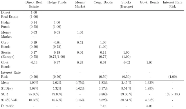
Table 2.1 depicts the empirical risk and return proles for the benchmark indices, as

well as the empirical and regulatory correlation matrices and the SCR. The upper

gures in the rst section of the table show the empirical correlations between the

returns of the benchmark indices. The gures in parentheses below show the reg-

Table 2.1: Descriptive Statistics and Solvency II Standard Formula Calibration

Direct Real

Estate Hedge Funds Money

Market Corp. Bonds Stocks

(Europe) Govt. Bonds Interest Rate Risk

Direct 1.00

Real Estate (1.00)

Hedge 0.14 1.00

Funds (0.75) (1.00)

Money 0.03 0.05 1.00

Market - - -

Corp 0.19 -0.04 0.52 1.00

Bonds (0.50) (0.75) - (1.00)

Stocks 0.47 0.18 0.06 0.14 1.00

(Europe) (0.75) (0.75/1.00) - (0.75) (1.00)

Govt. -0.13 0.37 0.29 0.07 -0.02 1.00

Bonds - - - -

Interest Rate - - - -

Risk (0.50) (0.50) - (0.50) (0.50) - (1.00)

Mean 1.90% 2.62% 0.75% 1.83% 2.45 % 1.33% -

STD(σ) 5.08% 5.32% 0.62% 3.17% 9.51 % 1.89% -

SCR 25.00% 49.00% - 8.86% 39.00 % - 1%×DG

99.5% VaR 18.38% 16.50% 0.15% 8.82% 38.84 % 4.31% -

Duration - - - 7.16 - 5.03 -

The upper division of the table shows the empirical correlation coecients and the regulatory correlation coecients (in parentheses below). All correlations refer to the downward interest rate shock scenario. Stocks and hedge funds are aggregated rst with a 0.75 correlation. The lower division of the table shows the mean quarterly returns of the assets and the corresponding standard deviations(σ). Moreover, the capital requirements (SCR) and the values at risk (VaR) as their empirical counterparts are presented. The interest rate risk's SCR must be calculated depending on the actual duration gap (DG). The respective durations for the assets are outlined in the last row.

ulatory correlations as imposed by EIOPA (2012). The second section of the table provides information on the mean quarterly returns, the standard deviations, the empirical VaR (on an annual basis) as well as the corresponding SCR, as already outlined in Section 3.2.

The descriptive statistics show the expected risk-return relationship for the bench- mark indices: Short-term money market instruments yield the lowest returns and also exhibit the lowest risk in terms of standard deviation. At the other extreme are stocks with a mean quarterly return of 2.45% and a standard deviation of 9.51%, thus representing the riskiest and best-yielding asset class, except for hedge funds.

The rather high capital requirements for high yielding assets (stocks, hedge funds

and real estate) indicate that certain target returns may no longer be attainable for

insurers with a low equity base, as already conjectured in the introduction. More-

over, the SCR calculated by EIOPA in 2012 does not seem to be in line with its

empirical counterpart any longer. The indices we use show a value at risk of only

18.38% for real estate and only 16.50% for hedge funds, as opposed to 25% SCR and 49% SCR, respectively.

Similarly, the correlation gures imposed by the Solvency II standard formula severely overestimate the empirical correlations, which under- mines the incentive for a thorough portfolio diversication. The parameterization of the standard formula may therefore not only render certain target returns unattain- able, but may also lead to inecient portfolio allocations and increase investment risk, instead of mitigating risk.

In the next section, we further analyze the eects of the potentially incorrectly parameterized capital requirements of the Solvency II standard formula in a dynamic portfolio optimization context.

2.4 Portfolio Optimization

2.4.1 Attainability of Target Returns and Portfolio Eciency

The attainable target return as a function of insurers' basic own funds is obtained by solving the well-known quadratic portfolio optimization program, as rst intro- duced by Markowitz (1952). The covariance matrix (Σ

) is comprised of capital requirements (SCR) and regulatory-imposed correlations, instead of empirical stan-

10

In accordance with the EIOPA framework, the value at risk was calculated on an annual basis

for the 99.5% level.

dard deviations (σ) and empirical correlations.

The optimization program can be stated as follows:

min

: SCR

= p

w

Σ

w, (2.11)

subject to w

M = µ

, (2.12)

w

≥ 0, (2.13)

w

1 = 1, (2.14)

and w

≤ u

i ∈ {1, 2, . . . , 6}, (2.15)

where:

• w

is the weight of asset class i ,

• w is the column vector of portfolio weights,

• M is the column vector of mean returns, and

• u

is the upper limit for the weight of asset class i .

The optimization objective is to minimize the portfolio's SCR with respect to a given target return (Equations 2.11 and 2.12). Equation 2.13 excludes short positions, and Equation 2.14 constrains the budget. In addition, Equation 2.15 introduces

11

The Solvency II covariance matrix is calculated as the outer product of the regulatory cor- relation matrix (R

) and the column vector of capital requirements (SCR), both as shown in Table 2.1 (Σ

= SCR ⊗ R

⊗ SCR

) . The resulting matrix is not positive semi-denite, which may cause a discontinuity in the quadratic objective function (Equation 2.11). We therefore ap- ply the algorithm of Higham (2002) in order to obtain the nearest positive semi-denite matrix.

Furthermore, there are circularity issues: Both the equity SCR and the interest rate SCR are a

function of the portfolio weights themselves (i.e., a function of the solution vector of the optimiza-

tion program). While the equity SCR accounts for diversication within the equity sub-module,

the interest rate SCR is determined by the duration gap, which in turn depends on the weights of

corporate bonds and government bonds. To overcome these issues, all N permissible combinations

of hedge funds, stocks, corporate bonds and government bonds are enumerated up to the fourth

decimal place. For any given target return, the original problem is now solved N times. Each of

the N optimizations uses the corresponding preset asset weights as additional constraints (i.e., the

weights of the four asset classes with circularity issues are held constant). Hence, the covariance

matrix no longer exhibits circular references. Finally, the portfolio allocation with the lowest SCR

of all the N optimization results is chosen as the global optimum for the respective target return.

investment limits to ensure that only realistic portfolios are obtained. The limits are derived from previous European regulatory standards, which are still reected in the actual portfolios of European insurers.

Specically, real estate weights are capped at 25%, hedge fund weights at 5%, stocks at 35% and equities (hedge funds and stocks together) are not allowed to exceed 35% of total assets.

The optimization program is solved for all achievable target returns.

The resulting portfolios exhibit the lowest possible capital charges for any given target return. The results likewise show the maximum attainable target return for any given SCR (i.e., any exogenously given amount of basic own funds). The attainability of portfolio eciency depending on the insurers' basic own funds is derived in a straightforward way. We run the portfolio optimization program as described by Equations 2.11 to 2.15, replacing the regulatory covariance matrix (Σ

) with the empirical covariance matrix (Σ

) in order to obtain the set of mean-variance-ecient portfolios. Sub- sequently, we calculate the SCR induced by the mean-variance-ecient portfolios, using Formula 2.10.

Figure 2.1 illustrates the results of both optimization programs in the µ -SCR-space.

The SCR-optimal frontier is plotted as a solid line, while the mean-variance-ecient portfolios are plotted as a dashed line. It is obvious that the SCR-optimal portfolios lead to much lower capital requirements than the mean-variance-ecient portfolios.

In other words, almost any target return is attainable with a much lower amount of basic own funds if the insurer strictly adheres to the Solvency II standard formula instead of minimizing investment risk. This rst result already shows the incom- patibility between actual investment risk and the market risk capital requirements according to Solvency II. Moreover, the asset allocations and the investment risk dif- fer decisively between the results of both optimization programs. The SCR-optimal

12

The investment limits we use are particularly inspired by the German Regulation on the Investment of Restricted Assets of Insurance Undertakings (Investment Regulation; German:

Anlageverordnung).

13

The lowest portfolio target return is determined by the asset class with the lowest expected

return, i.e., money market. At the other extreme, the highest portfolio target return is achieved by

sequentially increasing the weights of the assets with higher expected returns, until the individual

investment limits are reached.

Figure 2.1: Optimized Portfolios in the µ -SCR-Space

See text for explanations.

frontier is characterized by four points, which are depicted in Figure 2.1: The Min- SCR-portfolio at the lower left end of the curve consists of 100% government bonds.

This is not surprising, since government bonds have no SCR as such, but they have

a duration of 5.03, which enables them to hedge insurers' liabilities against interest

rate shocks. The portfolio at point 2 consists of 100% corporate bonds. Corporate

bonds have comparably low capital requirements, but also have very good abilities

to hedge liabilities against interest rate shocks (a duration of 7.16). At point 3, the

portfolio consists of 65% corporate bonds, 30% stocks and 5% hedge funds. This

portfolio at point 4 has the maximum achievable target return given the investment

limits ( µ = 2.07%, SCR = 25.42). The portfolio consists of 40% corporate bonds,

30% stocks, 5% hedge funds and 25% direct real estate. The concave curvature be-

tween the four knit points indicates that the Solvency II standard formula accounts

for some diversication in terms of capital charges. However, compared to the com-

mon Markowitz optimization, the diversication eect is negligible, and clearly does

not govern the allocation process. The allocation is clearly driven by the asset

classes' capital charges and durations. The asset classes are allocated sequentially

without noteworthy diversication. Asset classes with high capital requirements are allocated only when required by the target return.

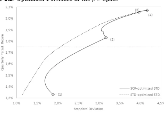
The mean-variance-ecient portfolios also consist of government bonds and cor- porate bonds to a large extent, as the returns of these asset classes exhibit low volatility. However, stocks, hedge funds and real estate are now allocated across the entire spectrum of target returns. In contrast to the SCR-optimal portfolios, the asset classes are now allocated simultaneously, not sequentially. The allocation is governed by the diversication eect instead of the duration gap. Appendix 1 shows the asset allocations for both optimization programs' results in detail. Figure 2.2 illustrates the results of both optimization programs in the µ − σ -space and mani- fests the deadweight loss caused by the Solvency II standard formula: Given a target return of 1.75%, the standard deviation of the mean-variance-ecient portfolio is 75 basis points below the corresponding standard deviation of the SCR-optimal port- folio. Using two standard deviations as the relevant measure for quantifying risk, the shortfall risk of the portfolio would increase decisively by 150 basis points per quarter!

As Figure 2.2 shows, the dead weight loss becomes even larger for higher target returns.

According to the information provided by the German Federal Financial Supervisory Authority (BaFin) and the results of QIS5 released by EIOPA (2011), the average European insurer's basic own funds amount to approximately 10%-12%. In the spirit of Braun et al. (2015) and Hoering (2013), we use 12% as a reference point for the further analysis. Considering the average European insurer's asset allocation in the past (see, e.g., Fitch Ratings, 2011; Insurance Europe and Oliver Wyman, 2013), as well as the past performance of the asset classes, the quarterly target return used to be approximately 1.75% (or 7% p.a.). This is sucient to cover the high interest rate guarantees on existing insurance policies and additional overhead costs.

As the vertical gridline in Figure 2.1 shows, quarterly returns of up to 1.88% are at-

14

This corresponds to a value at risk of approximately 95%, assuming returns are normally,

identically and independently distributed.

Figure 2.2: Optimized Portfolios in the µ - σ -Space

See text for explanations.

tainable with basic own funds of 12%. However, only 1.68% are eciently attainable.

The ecient portfolio with a 1.75% quarterly return induces an SCR of 13.45%. This

result shows that average and overcapitalized European insurers are well equipped

to fulll the capital requirements according to the Solvency II standard formula and

minimize their portfolios' investment risk at the same time. However, the situation

turns out dierently for undercapitalized market participants. According to the

QIS5 results of EIOPA (2011), one-quarter of all European insurers are at risk of

not meeting the capital requirements imposed by Solvency II. Putting aside opera-

tional risks (e.g., insucient reinsurance or high concentration risk), it is likely that

these insurers' basic own funds amount to less than 12%. As Figure 2.1 shows, the

attainable target return decreases sharply for insurers with basic own funds below

10%. The eciently attainable target return decreases even more rapidly. Portfolio

eciency is not attainable at all for insurers with basic own funds below 10%. Un-

dercapitalized insurers will not be able to increase their allocations of equities and

alternative assets in the search for higher returns and portfolio diversication. On

the contrary, undercapitalized insurers might be forced to reduce these asset classes

in order to match their portfolio's capital requirement with their basic own funds.

In the next section, we analyze how the optimal portfolio weights for the individual asset classes respond to a restriction on insurers' basic own funds.

2.4.2 Eects on the Allocations of Individual Asset Classes

The optimization programs run in Section 4.1 can be considered as extreme points.

No insurer will strictly adhere to only one of the optimization objectives (SCR or standard deviation). Rather, in practice, it is the combination of both optimiza- tions that is of particular relevance. We therefore include the insurers' basic own funds as an additional constraint into the standard mean-variance optimization. The optimization program is now formulated as follows:

min

: σ = p

w

Σ

w, (2.16)

subject to w

M = µ

, (2.17)

w

≥ 0, (2.18)

w

1 = 1, (2.19)

w

≤ u

i ∈ {1, 2, . . . , 6}, (2.20)

and BOF = p

w

Σ

w, (2.21)

where:

• BOF is the basic own funds of the insurer.

Equation 2.21 ensures that the resulting SCR (right-hand side) stays below the

insurer's basic own funds (left-hand side), while the portfolios are optimized with

regard to investment risk (Equation 2.16). The BOF serves as an upper boundary,

and is given exogenously by the equity capital of the individual insurer. By varying the BOF, it is now possible to derive the optimal portfolio allocation for any given combination of capital budget and target return.

The optimization program is solved for all achievable target returns and for four dierent levels of BOF (8%, 10%, 12% and 14%). The six panels depicted in Figure 2.3 show the target returns on the horizontal axis, and the respective asset weights on the vertical axis. The four levels of basic own funds are indicated by the legends underneath the respective panels. In addition, the unrestricted portfolio weights are shown as solid black lines and the quarterly target return of 1.75% is indicated by the vertical grid line.

When interpreting the results for a quarterly target return of 1.75%, it becomes evident that stocks, hedge funds and real estate allocations react extremely sensi- tively to a restriction on insurers' basic own funds. Government bonds are robust to variations in the BOF, and corporate bond allocations do even increase after the basic own funds have been restricted. For high target returns, money market in- struments are not a part of the ecient portfolios at all. The results show that the introduction of Solvency II will indeed reverse the trend towards higher quotas for stocks and alternative investments, especially for insurers with a weak equity base.

Insurers with basic own funds below 10%, for example, are forced into real estate

quotas below 5% and hedge fund allocations below 2%.

Figure 2.3: Optimal Portfolio Allocations for Dierent Levels of Basic Own Funds

Panel a: Allocation of Stocks Panel b: Allocation of Money Market Instruments

Panel c: Allocation of Hedge Funds Panel d: Allocation of Direct Real Estate

Panel e: Allocation of Government

Bonds Panel f: Allocation of Corporate

Bonds

Figure 2.3 illustrates the STD-optimal portfolio weights for the six asset classes for dierent given levels of basic own funds. The unrestricted portfolio weights are shown as the solid black line, and the quarterly target return of 1.75% is indicated by the dot-dashed vertical gridline.

2.5 Conclusion

In 2016, the EIOPA introduced a risk-based capital model for European insurers (Solvency II), and thereby changed the set of rules that had prevailed for previous decades. To analyze the eects of the new regulatory standard on insurers' invest- ment strategy, we conducted several portfolio optimization programs with respect to the capital requirements of the Solvency II standard formula.

Our results show that the Solvency II capital requirements impede the construc- tion of mean-variance-ecient portfolios. There are three main reasons for this: (1) The Solvency II standard formula presets very high correlations between the asset classes, and therefore does not reward risk reduction through diversication, (2) the solvency capital requirements for equities and for alternative asset classes are set too high, and (3) Solvency II focuses on the mitigation of interest rate risk, in contrast to the classical mean-variance optimization. While the latter can be deemed economi- cally meaningful, the rst two issues must be considered as misspecications of the Solvency II standard formula. The high regulatory correlation gures and capital requirements for real estate and equities (including hedge funds) may be the result of a principle of prudence, which is reasonable when viewed in isolation. However, with a holistic view, unbalanced and inecient portfolios are the consequence.

As a consequence, Solvency II increases the portfolios' investment risk and decreases

the attainable target return for insurers with a weak equity base. Given that the

primary purpose of the regulation is the mitigation of risk, and given that some

insurers are already facing an undercoverage in terms of returns, those eects are

highly undesirable. However, insurers with above-average amounts of basic own

funds (12% or higher) are able to fulll the Solvency II capital requirements, at-

tain high target returns and attain mean-variance-eciency at the same time (see

Figure 2.1). Those insurers do not face a binding constraint with the introduction

of the Solvency II capital requirements, as Hoering (2013) stated. On the other

hand, insurers with below-average basic own funds (10% or lower) are limited in

their attainable target returns. Furthermore, those insurers are not able to attain mean-variance-eciency irrespective of the target return (see Figure 2.1). Undercap- italized insurers are forced to strictly minimize the SCR according to the Solvency II standard formula when constructing their portfolios. As Figure 2.2 illustrates, this increases investment risk in the classical sense and might cause severe asset management biases, as stated by Braun et al. (2015).

Technically, the Solvency II standard formula forces insurers with a weak equity base

to reduce assets with a high SCR and no interest rate sensitivity, namely stocks,

direct real estate and hedge funds (and presumably all other investments in the

equity risk sub-module, in particular type 2 equities). Small and mid-size insurers

with a weak equity base are not able to develop and audit a cost-intensive insurance

internal solvency model to evade the standard formula. The regulator could mitigate

this issue in the future by allowing for more exibility when considering revisions to

the standard formula.

2.6 Appendix 1

Figure 2.4: Optimal Portfolio Allocations

Panel a: Optimal Allocations for SCR-optimized Portfolios

Panel b: Optimal Allocations for STD-optimized Portfolios

Figure 2.4 shows the resulting asset allocation for both optimization programs as stated in Section 2.4.1.

Chapter 3

The Determinants of Real Estate Fund Closures

Sebastian Schnejdar, Michael Heinrich, Rene-Ojas Wolter- ing, Steffen Sebastian

33

3.1 Introduction

With invested capital of EUR 145 billion, the German open-end real estate fund industry is the predominant indirect German real estate investment vehicle and the largest market for open-end real estate funds worldwide.

Investors in open-end real estate funds trade with the fund's investment company, which sells and redeems shares at net asset value (NAV) on a regular basis. The open-end structure is associated with considerable bank run risk (i.e., fund run risk), because of the long-term direct real estate investments and daily share re- demptions (Bannier et al., 2008; Weistroer and Sebastian, 2015; Fecht and Wedow, 2014). Therefore, German regulation demands a minimum liquidity reserve of 5% of a fund's NAV. In practice, average liquidity ratios range from 20%-30% (see Downs et al., 2016). Nevertheless, these liquidity ratios occasionally prove insucient, es- pecially during times of high volatility.

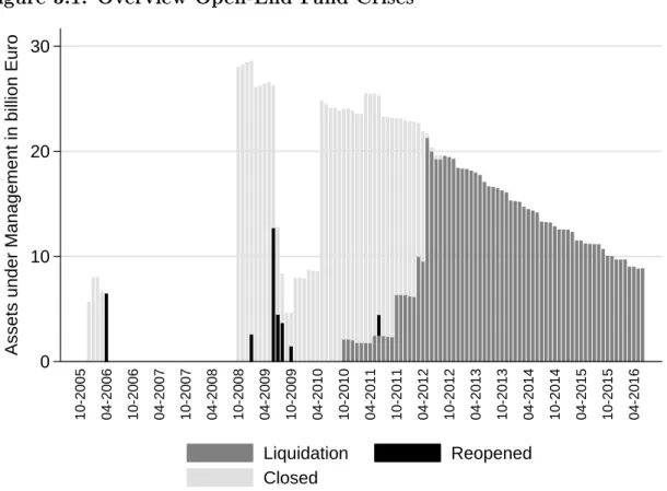
The German open-end fund industry was hit severely in the aftermath of the global nancial crisis. As of October 2008, ten public German open-end real estate funds with total assets under management of about EUR 28 billion were forced to suspend share redemption.

We use a panel logit model to explain fund closure probability. Our empirical study is based on a monthly panel dataset that consists of twenty-four open-end German real estate retail funds, and which covers all closure events in the history of the asset class.

We nd that fund closure probability increases with increasing fund run risk, which is represented by a fund`s liquidity ratio and net capital inows. Economies of scale and

1

Downs et al. (2016).

2

The regulatory regime was modied in succession of the fund crisis. Nevertheless, our analysis is unaected by those changes, since fund closure events occurred under the prior investment law (InvG, eective from January 1, 2004-July 22, 2013).

3

In our sample, we focus on retail funds. We exclude semi-institutional funds, which are

primarily intended for institutional investors. Semi-institutional funds are legally classied as

retail funds, but the minimum investment ranges from EUR 10,000 to EUR 1 million.

scope, proxied by fund size, age, and the presence of a distribution network for fund shares, help prevent fund closures. Moreover, we nd evidence that industrywide spillover eects from the closure of other open-end real estate funds tend to increase fund closure probability. Lastly, we nd evidence that a larger share of institutional investors increases fund closure probability.

Identifying fund closure determinants helps diminish uncertainty about the overall asset class, while restoring trust in the remaining funds.

The most recent example of a fund crisis was the massive share redemptions from U.K. open-end real estate funds that took place in the aftermath of the Brexit referendum on June 23, 2016. Seven public open-end funds from the U.K. closed, which represented one-half the total assets under management of the U.K. market.

Hence, open-end fund participants in foreign countries like the U.K. could learn from the German experience.

The paper is structured as follows. The next section (Section 3.2) gives an overview of the German open-end fund crisis. Section 3.3 describes the used variables, which are mainly derived from the existing literature of business failure prediction mod- els. Section 3.4 illustrates the dataset, while the regression results are presented in section 3.5. The last section exhibits our conclusion.

3.2 The German Open-End Fund Crisis

German open-end real estate funds are required by law to close (i.e., suspend share redemptions) if liquidity ratios fall below 5%. A shortfall in the fund liquidity ratio is very serious because open-end real estate funds are obliged to sell their real estate assets within the rst six months of closure without a discount to the last appraisal

4

M&G Property Portfolio, Henderson UK Property PAIF, Standard Life UK Real Estate Fund,

Aviva Investors Property Trust, Columbia Threadneedle UK Property Authorised Investment Fund

(PAIF), Canada Life UK Property Fund, and Aberdeen UK Property Fund.

value. Closed funds must sell sucient assets to raise their cash reserves and fulll share redemptions (i.e., reopen).

After a twenty-four-month period, funds are forced to sell o their entire real es- tate portfolios and pay out the proceeds to investors. However, selling properties during times of market turmoil, especially in the rst months of closure, is almost impossible. Hence, all the funds that closed in October 2008 were ultimately forced to liquidate after the twenty-four-month period. Nevertheless, seven of these funds reopened subsequent to their rst close in October 2008, but all were forced to close for good for a second time.

Figure 3.1 shows the size of closed German open-end real estate funds (grey bars), as well as the size of funds in liquidation (dark grey bars). The graph also illustrates the size of fund reopenings (black bars). During the rst fund crisis in 2005/2006, two open-end real estate retail funds with total fund volume of EUR 8 billion, closed.

These closures were caused by short-term uncertainty about the funds' property

valuations. After a short period of time, both funds reopened. The second, and

larger, crisis began in October 2008, with the closure of ten funds, with assets

under management of about EUR 28 billion. The reopening of several funds over

the following twelve months suggested an upward trend. Nevertheless all of these

funds were forced to close again. As of May 2010, the total fund size of distressed

funds was equal to earlier levels of around EUR 27 billion. Following the rst fund

liquidation announcement in October 2010, and through August 2012, all previously

closed funds were forced to announce their liquidations. The decreasing fund size

over the sample period, as shown in Figure 3.1, is due to two primary eects: 1) The

proceeds from distressed funds' sold properties were distributed to investors, and 2)

a decrease in property appraisal values. As of June 2016, about EUR 10 billion of

invested capital remained inaccessible to investors.