distributions and their relationships in the Southern Ocean, southeast

Characteristics of the surface water DMS and pCO

2

distributions and their relationships in the Southern Ocean, southeast

Indian Ocean, and northwest Pacific Ocean

Miming Zhang¹ , C. A. Marandino², Liqi Chen¹ , Heng Sun¹, Zhongyong Gao¹, Keyhong Park³, Intae Kim⁴, Bo Yang⁵ , Tingting Zhu⁶, Jinpei Yan¹, and Jianjun Wang¹

1Key Laboratory of Global change and Marine-Atmospheric Chemistry, Third Institute of Oceanography, State Oceanic Administration, Xiamen, China,²Forschungsberech Marine Biogeochemie, GEOMAR Helmholtz-Zentrum für

Ozeanforschung Kiel, Germany,³Division of Polar Ocean Science, Korea Polar Research Institute, Incheon, South Korea,

4Marine Radionuclide Research Center, Korea Institute of Ocean Science and Technology, Ansan, South Korea,⁵School of Oceanography, University of Washington, Seattle, Washington, USA,⁶State Key laboratory of Information Engineering in Surveying, Mapping and Remote Sensing (LIESMARS), Wuhan University, Wuhan, China

Abstract

Oceanic dimethyl sulfide (DMS) is of interest due to its critical influence on atmospheric sulfur compounds in the marine atmosphere and its hypothesized significant role in global climate.

High-resolution shipboard underway measurements of surface seawater DMS and the partial pressure of carbon dioxide (pCO₂) were conducted in the Atlantic Ocean and Indian Ocean sectors of the Southern Ocean (SO), the southeast Indian Ocean, and the northwest Pacific Ocean from February to April 2014 during the 30th Chinese Antarctic Research Expedition. The SO, particularly in the region south of 58°S, had the highest mean surface seawater DMS concentration of 4.1 ± 8.3 nM (ranged from 0.1 to 73.2 nM) and lowest mean seawaterpCO₂level of 337 ± 50μatm (ranged from 221 to 411μatm) over the entire cruise. Significant variations of surface seawater DMS andpCO₂in the seasonal ice zone (SIZ) of SO were observed, which are mainly controlled by biological process and sea ice activity. We found a significant negative relationship between DMS andpCO₂in the SO SIZ using 0.1° resolution, [DMS]_seawater=0.160 [pCO₂]_seawater + 61.3 (r² = 0.594,n= 924,p<0.001). We anticipate that the relationship may possibly be utilized to reconstruct the surface seawater DMS climatology in the SO SIZ. Further studies are necessary to improve the universality of this approach.

1. Introduction

The Southern Ocean (SO) exerts a strong influence on global biogeochemical cycles and air-sea gasfluxes [Tortell and Long, 2009]. It has been identified as a strong sink for atmospheric CO₂ [Landschützer et al., 2015;Sabine et al., 2004] and a significant source for the climate-active gas dimethyl sulfide (DMS) in regions south of 50°S [Curran and Jones, 2000;Inomata et al., 2006;Kettle et al., 1999;Lana et al., 2011]. Emissions of Anthropogenic CO₂to the atmosphere are resulting in a relentless and significant rise in global temperature [Allen et al., 2009] and an unprecedented increase in ocean acidity [Caldeira and Wickett, 2003], while DMS emitted from the ocean is speculated to have a cooling effect due to its impact on particle and cloud conden- sation nuclei number concentrations [Charlson et al., 1987;Vogt and Liss, 2009]. Therefore, investigations for temporal and spatial distributions and air-sea exchange of DMS and CO₂in the SO will be necessary to further understand their influence on climate change.

Compared to other regions, the SO has been undersampled with respect to surface seawater DMS (south of 40°S, NOAA-Pacific Marine Environmental Laboratory (PMEL) DMS database, http://saga.pmel.noaa.gov.dms).

Most former studies in the SO relied on discrete sampling and lab measurements, which were time- consuming and insufficient for high-resolution observations [Berresheim, 1987;Curran et al., 1998;Inomata et al., 2006;Kiene et al., 2007;Staubes and Georgii, 1993]. Recently, the membrane inlet mass spectrometry has been used for high-resolution survey of DMS in the SO [Tortell and Long, 2009; Tortell et al., 2011, 2012]. They observed significant changes in surface seawater DMS andpCO₂over time scales of days to weeks and subkilometer spatial scales. However, these observations were generally conducted in polynyas along the coastal regions, such as Ross Sea and Amundsen Sea. Other important regions of the SO, particu- larly along the marginal ice zone (MIZ), where there is high phytoplankton biomass or primary production

Global Biogeochemical Cycles

RESEARCH ARTICLE

10.1002/2017GB005637

Key Points:

•The characteristics of surface water DMS andpCO2distributions from the Southern Ocean to northwest Pacific Ocean are investigated

•The correlations between DMS,pCO2, and environmental parameters are analyzed

•Anticorrelation between DMS and pCO2is found in the seasonal ice zone of the Southern Ocean

Supporting Information:

•Supporting Information S1

•Data Set S1

•Data Set S2

Correspondence to:

M. Zhang and L. Chen, zhangmiming@tio.org.cn;

liqichen@tio.org.cn

Citation:

Zhang, M., et al. (2017), Characteristics of the surface water DMS andpCO2

distributions and their relationships in the Southern Ocean, southeast Indian Ocean, and northwest Pacific Ocean, Global Biogeochem. Cycles,31, 1318–1331, doi:10.1002/

2017GB005637.

Received 8 FEB 2017 Accepted 6 AUG 2017

Accepted article online 11 AUG 2017 Published online 26 AUG 2017

©2017. American Geophysical Union.

All Rights Reserved.

[Ishii et al., 2002;Taylor et al., 2013;Park et al., 1999], are still lackingfine-resolution surface seawater DMS investigation.

Furthermore, it is hard to model surface DMS concentrations in the seasonal sea ice zone (SIZ) of the SO due to the scarcity offield measurements and the influence of sea ice dynamics on DMS concentrations [Lana et al., 2011]. On the other hand, remote sensing provides another way to estimate DMS concentrations by linking remotely sensed parameters like chlorophylla(Chla) and mixed layer depth (MLD) tofield-measured DMS concentrations [Simó and Dachs, 2002]. Recently,Kameyama et al. [2013] found evidence for a strong positive relationship between DMS and net community production (NCP) in the North Pacific Ocean. They anticipated that this relationship could be found in other regions with high primary production, such as the SO, and that surface seawater DMS concentrations could be reconstructed by the empirical relationship of DMS and NCP. Thus, it is possible that the DMS could be reconstructed by remotely derived NCP [Chang et al., 2014].

Indeed, there are two aspects related to the impact of the carbon system on sulfur biogeochemical cycling:

1. DMS concentrations appear to be sensitive to ocean acidification. Previous studies reported that seawater DMS concentrations were reduced under high seawaterpCO₂conditions [Park et al., 2014;Archer et al., 2013], and global DMS emissions may decrease as a result of bombined effects of ocean acidification and climate change [Six et al., 2013].

2. The relationship between primary production and sulfur compounds in natural seawater.Tortell and Long [2009] andTortell et al. [2011, 2012] investigated the relationships between DMS,pCO₂, andΔO₂/Ar (an index of NCP) in the SO polynyas. Their results indicated that DMS was strongly correlated withpCO₂ andΔO₂/Ar during spring in the Ross Sea but decoupled frompCO₂andΔO₂/Ar during summer in the Ross Sea and Amundsen Sea. As phytoplankton activity can strongly impact both the carbon cycle and sulfur cycle, linkages between the parameters of the carbon cycle and sulfur cycle seem reasonable.

At present, numerous SO surfacepCO₂data are available through the SOCAT database (http://www.socat.

info/). If sufficient numbers offield DMS measurements are available and the significant linkage between DMS and pCO₂is demonstrated, it is possible to develop an algorithm to reconstruct the surface DMS distribution using thepCO₂data from the SOCAT database. In this study, we performed high-resolution sur- face seawater DMS and pCO₂ measurements from the SO during the 30th Chinese Antarctic Research Expedition (CHINARE-Ant30th). The factors driving the surface DMS andpCO₂distributions were analyzed in the distinct oceanic regions. The relationship between DMS andpCO₂was also detailed and examined.

We propose that the relationship could be possibly used in the reconstruction of surface seawater DMS in SO SIZ.

2. Materials and Methods

2.1. Study Area

The SO is a typical high-nutrient and low-chlorophyll area due to iron (Fe) limitation [Boyd et al., 2000], in which primary production in the pelagic ocean is generally low with little variation [Arrigo et al., 1998].

However, in the SO SIZ, primary production exhibits great variability and it is strongly impacted by sea ice retreat and melting [Taylor et al., 2013;Smith and Comiso, 2008;Wang et al., 2014]. Particularly in the MIZ, phy- toplankton blooms are common. The MIZ has been associated with the retreating sea ice edge and is defined operationally as the area where sea ice is present at the beginning of the retreat but not at the end [Arrigo et al., 1998]. The variance of phytoplankton activity and sea ice conditions in the SO could certainly impact the biogeochemical cycle of gases, such as DMS and CO₂[Tortell and Long, 2009].

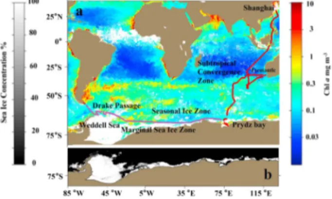
Our measurements were conducted on board theR/V Xue Long in February–April 2014 during CHINARE- Ant30th. The ship tracks were from Drake Passage, SO to the East China Sea (Leg 1, named as west-east transect: from Drake Passage to Prydz Bay, 7–24 February 2014; Leg 2, named as south-north transect: from Prydz Bay to Fremantle, Australia, 26 February to 16 March 2014, and from Fremantle, Australia, to East China Sea, 22 March to 11 April 2014). The entire cruise track was about 28,000 km and the main part of transect traversed the Atlantic Ocean Sector and Indian Ocean Sector of the SO. In general, most of the west-east transect was located in the MIZ (Figure 1).

2.2. Chemical Analyses

A custom-built automatic purge and trap system coupled with gas chromatography-pulsedflame photometric detection (Trace GC, Thermo Company, USA) was utilized for shipboard underway continuous measuring of surface seawater DMS. Details of the method and calibration proce- dure are described by Zhang and Chen[2015]. The surface seawater samples were continuously intro- duced to the analysis system through the ship’s seawater pump system at 4 m depth. The sample rate of this system is 10 min¹ and the detection limit is 0.05 nM.

The ship cruising speed was about 10–15 knots in sea ice areas, which led to a spatial sample resolution of 3–4.5 km.

An automatic system (GO Flow pCO₂system, Model 8050, General Oceanic Inc., Miami FL, USA) was installed on board for underway pCO₂observations, and calibration was done using CO₂ standard gases from National Oceanic and Atmospheric Administration (NOAA) with concentrations of 244.25, 366.86, and 546.98 ppmv (CO₂/air). The measurement method was the same as described inGao et al. [2012]. The sampling interval was about 3 min and the system was calibrated every 2.5 h. The accuracy was estimated to be better than 2 μatm for seawater pCO₂.

Sea surface temperature (SST) and salinity (SSS) were deter- mined continuously by the shipboard underway conductivity- temperature-depth system (SBE21, USA) at a sampling interval of 5 s.

In addition, meteorology data, such as wind speed and air pres- sure, were obtained from the ship- board meteorology observation system run by National Marine Environmental Forecasting Center of China. The GPS information was Figure 1.(a) The transect during the thirtieth Chinese National Antarctica

Research Expedition (purple line is the west-east transect; red line is the south-north transect). The background is the monthly averaged Chlacon- centration (color scale), and the white color represents areas where Chlais undetectable; (b) daily sea ice distribution along the transect from 9 to 28 February 2014 (gray scale).

Figure 2.The distribution of (a) surface seawater temperature (SST), salinity (SSS), sea ice concentration (grey); (b) monthly averaged NPP and EP; (c) MLD (grey) and wind speed; (d) DMS and monthly average Chla(red); (e) surface seawaterpCO₂, and atmosphericpCO₂in the west-east transect. Note that the data between the yellow lines are the high DMS levels located in the MIZ.

obtained from the shipboard GPS record, providing the sampling positions of DMS andpCO₂. 2.3. Acquisition of Remote Sensing Data

The 8 day and monthly average remotely sensed Chl a data were downloaded from the Aqua Moderate Resolution Imaging Spectroradiometer (MODIS) web- site (http://oceancolor.gsfc.nasa.

gov/) with a spatial resolution of 9 km. We did not use the daily data due to inconsistent data coverage over most of the ship track. We matched the 8 day and monthly average data with the DMS data obtained in thefield using latitude, longitude, and time of measure- ment, and made the comparison of the matching ratio (number of Chl a data matched/number of DMS data). When using 8 day aver- age Chladata, the matching ratios were 44.98% and 80.01% in west- east transect and south-north transect, respectively. More favor- able matching ratios, 82.39% and 90.16%, were achieved in west-east transect and south-north transect when using monthly average data.

Please also see the comparison between 8 day and monthly aver- age Chladata along the transects in the supporting information (Figure S1). We found that there is general agreement between them. Thus, we decided to use the monthly average Chlain west-east transect and 8 day average Chladata in south- north transect for our discussion.

The daily sea ice concentrations along the transects were obtain from the University of Bremen (http://www.

iup.uni-bremen.de:8084/amsr2/ and Figure 1), with a spatial resolution of 6.25 km [Spreen et al., 2008]. The sea ice concentration distributions were presented in Figures 2a and 3a along the transect. Most of the ship track in the SO is not far from the sea ice margin. There were only a few areas of the ship track with high sea ice concentrations due to the fact that the icebreaker usually avoided high sea ice concentration areas for safety concern. In addition, when the ship was in heavy sea ice conditions, the DMS andpCO₂observations were stopped to avoid potential damage to the water pump.

Mixed layer depth (MLD) has been shown to be an important parameter in reconstructing DMS concentra- tions at the surface ocean [Simó and Dachs, 2002]. Here we use the global monthly MLD climatology data from Institut Français de Recherche pour l’Exploitation de la Mer (http://www.ifremer.fr/cerweb/deboyer/

mld/Surface_Mixed_Layer_Depth.php) with a resolution of 2° × 2° grid, which was estimated from afixed threshold on density profiles [Clément et al., 2004].

MLD¼depth where σ0¼σ010mþ0:03 kg m³

(1) Figure 3.The distribution of (a) surface seawater temperature (SST),

salinity (SSS), sea ice concentration (grey); (b) monthly average NPP and EP;

(c) MLD (grey) and wind speed; (d) DMS and 8 day average Chla(red); (e) surface seawaterpCO₂(the atmosphericpCO₂was not measured) in the south-north transect.

The criterion selected is a threshold value of density from a near-surface value at 10 m depth (Δσθ = 0.03 kg m³). The MLD data in the south-north transect are correlated with the variation offield wind speed data (Figure 3), but the two values are not always correlated in the west-east transect (Figure 2). This may be explained by the fact that the MLD data are from monthly climatology, which may not represent thefield condition along the ship track.

Net primary production (NPP) is defined as the remaining photosynthetic products that are available for phytoplankton growth or consumption by the heterotrophic community. In the Vertically Generalized Production Model [Behrenfeld and Falkowski, 1997], oceanic NPP is a function of Chla, available light, and the photosynthetic efficiency. Monthly NPP data were obtained from the Ocean Productivity website (https://orca.science.oregonstate.edu), where the standard product is based on MODIS Chla, MODIS sea sur- face temperature, Sea-viewing Wide Field-of-view Sensor PAR (photosynthetically available radiation), and estimates of euphotic zone depth from a model developed byMorel and Berthon[1989]. The export produc- tion (EP), the portion of primary production driven by externally supplied nutrients (“new”production) when a steady state nutrient budget with a constant elemental organic matter stoichiometry is assumed for the euphotic zone [Dunne et al., 2005], was estimated as the following equation byLaws et al. [2011]:

Ef¼ðð0:58570:0165TÞpÞ=ð51:7þpÞ (2) Efis the EP to NPP ratio,Tis SST (°C), andpis the NPP in mg C m²d¹. Equation (2) accounts for 87% of the variance in the observedEfratios in global ocean [Laws et al., 2011]. The estimated EP and NPP data can be utilized to explain the surface seawater DMS andpCO₂variance.

3. Results and Discussion

3.1. Sea Ice Distribution and Surface Water Hydrography

Our study area consisted of two distinct transects: one was mainly located in the SO MIZ (west-east transect) and the other one traversed from the SO to the East China Sea (south-north transect). During the time of survey in the west-east transect, the sea ice melting rate was slow and the sea ice extent was close to the minimum level of the year. In the area south of 60°S (transect from 60°W to 75°E), SST and SSS varied from1.7°C to 1.0°C and from 34.2 to 32.8, respectively. In the SO, the temperature and salinity of surface water masses were significantly influenced by surface warming and sea ice melting. The waters with SST<0.5°C (black dash line in Figure 2a) and SSS<33.4 (red dash line in Figure 2a) were identified as a residual ice melt signals in these regions [Tortell et al., 2012]. The influence of sea ice melting on the surface waters was found along the west-east transect, where there were cold water areas (SST<0.5°C) associated with relatively low salinity (SSS<33.4). Around 50°E, we observed high sea ice concentrations corresponding with low-temperature and low-salinity seawater. In addition, we could notfind waters significantly impacted by circumpolar deep water (CDW, warm water with high salinity,T>1°C,S>34.7) along the transect.

In the south-north transect, a strong latitudinal gradient of SST (range from1.8°C to 30.9°C) and SSS (range from 31.3 to 35.9) was clearly visible (Figure 3). In general, SSS was more variable than SST along this transect.

A maximum SSS of 35.9 was found around 32°S and decreased both southward and northward. Thefluctua- tions in SSS in the Prydz Bay (~2) could be attributed to the formation of sea ice at the end of February, which could increase the salinity of seawater. Along the transect from 58°S to 42°S, SSS exhibited a small variance, while there was significant increase of SST from south to the north. These features are due to the eastward flow of the Antarctic Circumpolar Current (ACC), which is driven by the world’s strongest westerly winds (wind speed>10 m s¹). North of the ACC, from 32°S to 42°S, we observed a large change of SST (>5°C) and SSS (>0.5), which was identified as the Subtropical Front (STF) [Orsi et al., 1995] and Subtropical Convergence Zone (SCZ). In contrast, a noticeable decline of SSS at the equator was observed, likely due to the input of freshwater from continental runoff and rainfall. In the East China Sea, the observed decline of SSS and SST is the result of freshwater input from the Yangtze River.

3.2. The Distributions of Satellite Derived Chla, NPP, and EP

Distributions of Chl a, NPP, and EP along the transects are presented in Figures 2b, 2d, 3b, and 3d.

Monthly average Chl ain the west-east transect and 8 day average Chl ain south-north transect were

0.25 ± 0.19 mg m³(0.06–1.32 mg m³) and 0.18 ± 0.21 mg m³(0.01–1.92 mg m³), respectively, with variability similar to NPP and EP. The mean NPP and EP values were 155 ± 74 mg C m²d¹(range: 62– 415 mg C m²d¹), 69 ± 41 mg C m²d¹(range: 20–218 mg C m²d¹), and 439 ± 335 mg C m²d¹ (range: 78–3277 mg C m²d¹), 116 ± 122 mg C m²d¹(range: 12–1048 mg C m²d¹) in west-east and south-north transects, respectively.

In the west-east transect, significant variance of Chla, NPP, and EP was found and the high values were mostly located in the MIZ of Weddell Sea (40°W–50°W) and Indian Ocean Sector (35°W–15°E). The estimated NPP and EP in the MIZ are lower than the modeled monthly average primary production (PP) in the SO water from the study by Arrigo et al. [1998], in which relatively high PP values (750 mg C m² d¹ and 610 mg C m²d¹) were estimated in the MIZ of Weddell Sea and Indian Ocean Sector of SO in February.

In addition,Smith and Nelson[1990] reported that seasonal (from November to March) average new produc- tion in the MIZ of Weddell was at least 325 mg C m²d¹.

In the south-north transect, the relatively high Chla, NPP, and EP were found in the polynya of Prydz Bay, the MIZ around 60°S, the SCZ, and the East China Sea. NPP and EP values ranged from 523 to 1397 mg C m²d¹ and from 284 to 827 mg C m²d¹, respectively, in the polynya of Prydz Bay. Such high variability is likely due to the onset of sea ice formation around the polynya at the beginning of March, which has been shown to enhance phytoplankton biomass [Lizotte, 2001;Zhang et al., 2015]. The relatively high phytoplankton activity from 32°S to 42°S was located in the STF and SCZ, where the strong stratification and ample solar radiation caused the growth of phytoplankton [Llido et al., 2005]. The highest NPP and EP, with high Chla, were found in the East China Sea, where sufficient light and nutrients were the main factors that impacted phytoplankton activity.

3.3. Spatial Distributions of Surface Seawater DMS 3.3.1. West-East Transect

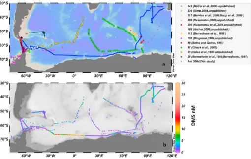
In the west-east transect, DMS concentrations exhibited large spatial variations with a mean value of 5.0 ± 9.7 nM, ranging from 0.1 to 73.2 nM (Figure 2a). The observations along the SIZ demonstrated that the distributions of DMS were not homogeneous. It is noteworthy that the observations from our cruise track filled the gaps of previous observations in the same region during the same time period (Figure 4).

As shown in Figure 4, our DMS data obtained along the transects were consistent with the previous observa- tions collected in the NOAA-PMEL DMS database. Clearly, large-scale high-DMS levels located in MIZ from 34°

Figure 4.Comparison of the surface seawater DMS data in this study with data from previous studies. (a) Sampling loca- tion. (b) DMS concentrations (shown with the color bar and note that the scale is capped at 30 nM to ensure readability of the plots). The previously acquired data were downloaded from NOAA-PMEL DMS database for the months of February and March. The chosen area was mostly located in the Indian Ocean sector and Atlantic Ocean sector of the SO.

W to 14°E was observed (Figure 4).

The position of this high DMS area was slightly east of that in the Lana et al. [2011] climatology for February. Our results were in agreement with many previous studies, in which high DMS levels commonly occur in the surface water of the MIZ [Curran et al., 1998; Inomata et al., 2006; Kettle et al., 1999], related to the high phytoplankton biomass there. The maximum DMS concentration dur- ing the cruise, 73.2 nM, was found around 3°E. This value is several times higher than previously reported values (27 nM [Turner et al., 1995], 22 nM [Curran et al., 1998], and 15.8 nM [Inomata et al., 2006]). However, it is lower than the observation of 88 nM in the MIZ of Weddell Sea byFogelqvist[1991]. The average Chl avalue in this large-scale high-DMS region (from 34°W to 14°E) drastically declined in the January, suggesting that high levels of DMS occurred after the bloom (Figure 5, black line). Microzooplankton grazing and massive death of algae can enhance the DMS concentration [Stefels et al., 2007]. In the later summer of the SO SIZ, diatoms (with low intracellular DMSP content) are likely the main phytoplankton species [Boyd, 2002]. These factors may explain the decoupling between the DMS and Chlahere.

Additionally, we found a DMS concentration peak (as high as 6.8 nM) around 50°E, corresponding with high sea ice concentrations. Previous studies have demonstrated that significant DMS and DMSP (dimethylsulpho- niopropionate, the precursor of DMS) levels (>100 nM) were observed under the sea ice bottom, coincident with very high Chlavalues [Trevena and Jones, 2012, 2006]. Addtionally, during the melting seasons, the DMS or DMSP from the sea ice bottom could be released into the surrounding waters. As described in section 3.1, we observed the influence of sea ice melt around 50°E; therefore, the high DMS levels there are likey be due to high DMS and DMSP concentrations in the sea ice.

3.3.2. South-North Transect

In the south-north transect, a distinct DMS distribution pattern in the different regions of the cruise track was observed (Figure 3d). Over the entire south-north transect DMS levels ranged from 0.2 nM to 16.9 nM with an average value 2.6 ± 1.6 nM.

High DMS concentrations (up to 9.8 nM), corresponding to high levels of Chla, were found near 40°S in the STF, where SSS was also high. The high DMS concentrations in the STF are similar to previous observations (Figure 4). High SSS in this region can increase intracellular DMSP production, possibly leading to high DMS levels [Stefels et al., 2007]. Moreover, the high irradiance there promotes shallower MLDs (~40 m), with consequences both for DMS release from stressed algal cells and inhibition of bacterial DMS consumption [Lizotte et al., 2012;Simó and Pedros-Alio, 1999;Vallina and Simó, 2007;Vila-Costa et al., 2014]. As shown in Figure 5 (red line), the average Chlain this high DMS area was invariable from January to May, suggesting that the DMS concentrations may be stable in this region.

The average DMS concentration between 15°S and 15°N was 2.4 ± 0.8 nM (range: 0.8 nM to 6.9 nM,n= 761).

The mean value is higher than that observed at the equatorial region of the west Pacific Ocean (mean value:

0.9 nM) [Zindler et al., 2013;Marandino et al., 2013], but it is in agreement with the measurements byBates and Quinn[1997], who reported that the surface seawater DMS mean level is relatively constant both seasonally and interannually (2.7 ± 0.7 nM) in the middle equatorial Pacific Ocean (15°S ~ 15°N) from 1982 to 1996.

DMS concentrations rapidly increased upon entry into the East China Sea, up to values of 16.9 nM (Figure 3d), coincident with variations in the Chlaconcentrations. High DMS levels in the surface water of the East China Figure 5.The variations of 8 day average Chlavalues in chosen regions from

January to May 2014. High levels of seawater DMS were found in these two regions. The arrows indicate the sampling time of DMS during this period.

Note that the average Chlavalues are calculated from averaging the satellite grid Chladata in Chosen regions.

Sea have also been observed in previous studies [Yang et al., 2012, 2011]. Additionally, the increase of DMS concentrations was also associated with a strong decrease of SSS and SST, indicating that the water input from Yangtze River may impact DMS concentrations [Yang et al., 2012].

3.4. Spatial Distributions of Surface SeawaterpCO₂

Surface seawater and airpCO₂levels were measured during the cruise (Figures 2e and 3e). The mean values of seawaterpCO₂were 347 ± 40μatm (221–411μatm) and 357 ± 39μatm (178–428μatm) in the west-east and south-north transects, respectively. The averagepCO₂^airwas 378 ± 4μatm in west-east transect, but pCO₂^air data were missing for the south-north transect. According to the computed values of ΔpCO₂ (pCO₂^seawater pCO₂^air), a critical parameter in the CO₂ air-seaflux calculation [Wanninkhof, 1992], the SO and East China Sea are a strong sink for atmospheric CO₂, while other regions of cruise track were identified as weak sinks or sources of atmospheric CO₂ (Table 1). Overall, the variation of pCO₂ during the cruise generally correlated with Chla, NPP, and EP.

Significant variations of surface seawaterpCO₂were found in the west-east transect (Figure 2e). These results are consistent with our previous campaign conducted in the SO [Chen et al., 2004], during which the distribu- tion ofpCO₂exhibited the same spatial distribution pattern. The strong atmospheric CO₂sink was found in the Atlantic Sector of the SO (34°W–14°E) due to the largeΔpCO₂and relatively high wind speed (Figures 4d and 4e).Stoll et al. [2002] also reported large-scale surface seawater CO₂undersaturation in the 65°S–70°S MIZ of the Atlantic Sector of the SO in austral summer, coinciding with high Chlacontent. Additionally, in the area west of 40°W, strikingly low seawaterpCO₂levels (down to 221μatm) were observed. The largestΔpCO₂in the west-east transect was simultaneously observed (157μatm). These low seawaterpCO₂levels may not only be impacted by biological activity but also melting sea ice (as SSS values<33.4 were observed). It has been reported that sea ice and its meltwater contain very low levels ofpCO₂[Cai et al., 2010]. The values mea- sured around 50°E (~360μatm) also appear to be impacted by meltwater, since the sea ice concentration was high and relatively low phytoplankton biomass was detected.

In the south-north transect, surface seawaterpCO₂levels presented relatively smaller variations than the west-east transect, except for the measurements in the Prydz Bay and East China Sea (Figure 3e). In the Prydz Bay, we found very low seawaterpCO₂levels, with a mean value of 198 ± 17μatm (n= 523), ranging from 178μatm to 258 μatm. The seawater pCO₂ increased with latitude until the heavy ice region was Table 1. The Mean Levels of DMS andpCO₂and Correlations Between DMS,pCO₂, Chla, NPP, EP, SST, SSS, Air Pressure (P) and Wind Speed (U, m s¹) in the Different Regions Outlined in the Text (Pearson Correlations)^a

Zones Mean Value Chla NPP EP SST SSS U DMS VersuspCO₂

≤58°SSIZ DMS 4.1 ± 8.3 0.395** 0.309** 0.309* 0.047 0.212** 0.303** 0.495**

n= 987

n= 2166 n= 978 n= 1160 n= 1159 n= 1164 n= 1164 n= 1012

pCO₂ 337 ± 50 0.682** 0.706** 0.730** 0.002 0.043 0.346**

n= 8592 n= 780 n= 945 n= 929 n= 930 n= 930 n= 804

58°S–42°SSAAZ DMS 2.4 ± 1.5 0.067 0.543** 0.427 0.607** 0.575** 0.010 0.245**

n= 143

n= 726 n= 161 n= 161 n= 161 n= 161 n= 161 n= 159

pCO₂ 362 ± 13 0.225** 0.749** 0.755** 0.706** 0.457 0.158

n= 2602 n= 143 n= 143 n= 143 n= 143 n= 143 n= 142

42°S–15°SSSCZ DMS 3.1 ± 1.8 0.765** 0.246** 0.689** 0.650** 0.048 0.066 0.494**

n= 263

n= 1882 n= 264 n= 268 n= 268 n= 268 n= 268 n= 268

pCO₂ 360 ± 10 0.607** 0.198** 0.367** 0.694** 0.266** 0.116

n= 5868 n= 259 n= 263 n= 263 n= 263 n= 263 n= 263

15°S–15°NEZ DMS 2.4 ± 0.8 0.052 0.078 0.063 0.376** 0.212 0.067 0.245**

n= 205

n= 761 n= 249 n= 270 n= 270 n= 274 n= 274 n= 267

pCO₂ 396 ± 12 0.003 0.005 0.009 0.078 0.463** 0.393**

n= 1976 n= 185 n= 201 n= 201 n= 205 n= 205 n= 198

15°N–30°NNSCZ DMS 2.2 ± 1.8 0.555** 0.374** 0.465* 0.378** 0.495** 0.165** 0.406**

n= 131

n= 395 n= 120 n= 140 n= 140 n= 140 n= 140 n= 140

pCO₂ 356 ± 42 0.691** 0.662** 0.725* 0.934** 0.317** 0.033

n= 1359 n= 114 n= 131 n= 131 n= 131 n= 131 n= 131

aThe number of samples is shown below the corresponding correlation.

*The correlation is significant at the 0.05 level (two tailed).

**The correlation is significant at the 0.01 level (two tailed).

crossed. The enhancement ofpCO₂there was in agreement with our previous study, and the upwelling of CDW around 64°S is likely the main reason [Gao et al., 2008]. Around 60°S, we observed a slight decrease of seawaterpCO₂(328μatm), which was associated with a Chlapeak. Between 42°S and 58°S, where wind speed was very high (>10 m s¹, Figure 3c), the seawaterpCO₂average value was 362 ± 13μatm, indicating a weak sink for atmospheric CO₂(Table 1). The values are similar to those measured in previous studies [Metzl et al., 1999, 1991;Poisson et al., 1993]. In the region around 40°S (STF), a large-scale feature of slightly low sea- waterpCO₂levels (average value: 346 ± 4μatm,n= 679, range: 335μatm to 365μatm) was found, which was not only coincident with the relatively high Chlabut also with relatively high SST. North of the SCZ, seawater pCO₂gradually increased and it exceeded the atmosphericpCO₂level (approximately 380μatm) in the equa- torial region. The average seawaterpCO₂in the equatorial region between 15°S and 15°N was 397 ± 11μatm, ranging from 361μatm to 428μatm (n= 2369), suggesting that the equatorial region is a significant source of CO₂to the atmosphere. The seawaterpCO₂levels started decreasing again around 20°N, and the lowest sea- waterpCO₂levels on this transect were found in the East China Sea (196μatm).

3.5. Correlations Between DMS,pCO₂, and the Environmental Parameters

The values of DMS,pCO₂, Chla, NPP, EP, SST, SSS, and wind speed were binned by 0.1° along longitude (west- east transect) or latitude (south-north transect) and correlated with each other (Table 1). Chla, NPP, and EP data were obtained using a remote sensing method, and the other parameters were measured directly on board. We separated the data intofive zones: (1) The region south of 58°S (≤58°S), most of which is located in the SO SIZ (named as SIZ); (2) The region between 58°S and 42°S, located in the sub-Antarctic zone and Antarctic zone (named as SAAZ) [Curran et al., 1998]; (3) The region between 42°S and 15°S located in the south SCZ (named as SSCZ); (4) The region between 15°S and 15°N, located in the equatorial zone as indi- cated byBates and Quinn[1997] (named as EZ); and (5) The region between 15°N and 30°N, located in the north SCZ (named as NSCZ).

We found that DMS and Chlaare significantly positively correlated in the SSCZ region (r= 0.765,p<0.01), moderately positively correlated in the NSCZ (r= 0.555,p<0.01), and weakly positively correlated in the SIZ (r= 0.395,p<0.01) but not correlated in the SAAZ and EZ regions. These results are consistent with the majority of publications indicating that the relationship between seawater DMS and Chlais not always straightforward in the oceans. Therefore, the relationship between Chlaand DMS cannot be used to predict DMS distributions in the global ocean. We found that DMS is significantly correlated with EP (r= 0.689, p<0.01) in the SSCZ region, but in the other regions, only weak positive correlations or no relationships were found. In the case of relationships between DMS and NPP, no correlations or weak positive correlations were computed in all regions. Although the high DMS levels are consistent with the high values of NPP and EP in the high production regions, the overall low linear correlations seem to disagree with the findings of Kameyama et al. [2013]. Additionally, our result in the SO is consistent with thefindings during the SO sum- mer, in which the DMS concentrations were not correlated withΔO₂/Ar (an index of NCP) [Tortell et al., 2011].

In the SIZ and SAAZ regions, the surface seawaterpCO₂values are significantly negatively correlated with NPP and EP (r > 0.7, p< 0.01). However, pCO₂ levels are strongly associated with Chla (r = 0.682, p<0.01) in the SIZ but weakly negatively correlated with Chlain the SAAZ region (r=0.225,p<0.01).

The results demonstrate that surface seawaterpCO₂was strongly impacted by biological activity in the SO [Takahashi et al., 2002]. In contrast, we found that seawaterpCO₂was not only significantly correlated with phytoplankton biomass but also strongly associated with SST in both the SSCZ and NSCZ regions, indicating that SST was also an important factor. The rising temperature can cause the decrease of the CO₂solubility, thereby increasing thepCO₂levels [Takahashi et al., 1993]. However, in the equatorial region, we could not find correlations between seawaterpCO₂and any other parameters.

3.6. Relationships Between DMS andpCO₂

Comparison of the concentration variations for DMS andpCO₂shows that they tended to vary inversely (Figures 2 and 3).Tortell and Long[2009] andTortell et al. [2011, 2012] observed a large range of correlations between DMS andpCO₂in the SO (rvalue ranged from0.03 to0.73). In this study, we also investigated the relationship between the DMS andpCO₂in different oceanic regions. As shown in Table 1, moderate negative correlations between DMS andpCO₂are found in the SIZ (r=0.495,n= 987,p<0.01), SSCZ (r=0.494, n= 263,p<0.01), and NSCZ (r=0.406,n= 131,p<0.01), while low negative correlations are found in

the SAAZ and EZ. The results show that the DMS andpCO₂correlations are different between the oceanic regions, with the high productivity regions having higher correlation values, such as in the SO SIZ and SSCZ. The correlation between DMS andpCO₂is better than the correlations between DMS and the other parameters in SO SIZ. This indicates thatpCO₂is a better predictor of DMS concentrations than Chlathere (Table 1, see the supporting information Figure S2). Therefore, we provide a more detailed investigation of the DMS andpCO₂relationship in the SO SIZ.

In the case of the SIZ (Figure 6), the data were divided into four clusters according to the biogeochemical characteristics: (1) high DMS levels and moderatepCO₂levels with high Chla(purple triangles) located in the region from 34°W–14°E, (2) low DMS and lowpCO₂levels with relatively high Chla(green diamonds) located in Prydz Bay and 43°W–45°W, (3) sea ice influence with low Chla(brown inverted triangles) located near 50°E, and (4) the remainder of the data (blue squares) with low DMS, highpCO₂, and relatively low Chla.

These clusters represent most of the DMS andpCO₂relationships in the SO SIZ. We found that there are two outlier data sets that deviate from the bulk of the data (Figure 6b, the data in red circles). One is characterized by DMS values above 40 nM, and the other one is characterized bypCO₂levels below 280μatm. The high DMS values with moderatepCO₂(DMS>40 nM) are likely located in the bloom-declining region (from 2°E to 4°E). Larger-scale algae death and possibly zooplankton grazing, in addition to microbiological processes, could rapidly enhance the seawater DMS concentrations. However, thepCO₂levels have little variance here, likely due to the fact that there is no longer active photosynthesis. The other cluster contains very lowpCO₂ levels with low DMS concentrations (green diamond) mainly locating in 43°W–45°W and Prydz Bay. The pro- duction of DMS is likely limited at that time due to the dominance of low DMSP-containing algae and/or low Figure 6.(a) DMS,pCO₂, and Chlain the SIZ. The color bar indicates Chlaconcentrations in mg m³. Relationships between DMS and (b)pCO₂binned to 0.1°; (c) temperature normalized (n-pCO₂) binned to 0.1°. Note that the data in the red circles are the outlier data.

microbial activity. In addition, lowpCO₂levels may be caused by both the uptake by phytoplankton, as well as the sea ice meltwater contribution (e.g., in the region 43°W–45°W).

After excluding the data in the red circles, a significant negative correlation between DMS andpCO₂was observed (r²= 0.594,n= 924,p<0.01) in the SIZ,

½DMSseawater¼ 0:160½pCO₂seawaterþ61:3 (3)

The relationship between DMS andpCO₂indicates that they have similar controlling factors in the ocean surface, namely, biological activity, air-sea exchange, and sea ice influence. These factors inversely affect the surface ocean DMS andpCO₂values. For example, high phytoplankton biomass can strongly uptake the CO₂in seawater while simultaneously producing the precursor of DMS. In addition, air-sea exchange only acts as a sink of the seawater DMS but is a source of seawater CO₂when thepCO₂levels in seawater are below the atmospheric CO₂levels. Finally, as stated above, sea ice melt may enhance DMS concentrations in vicinity waters but dilute the CO₂contents there.

As described inKameyama et al. [2014], the temperature effect calibration ofpCO₂, i.e., n-pCO₂, was used as the index of NCP, and they identified a significant negative correlation (r² = 0.59,n = 1263, P<0.001) between isoprene (a biogenic trace gas) and the n-pCO₂ in the SO. Therefore, the relationship between DMS and temperature-normalizedpCO₂(n-pCO₂) was also investigated, and it was also compared with the nonnormalized values. The temperature effect calibration was done according to the studies by Kameyama et al. [2014] andTakahashi et al. [1993] as the following:

npCO₂¼pCO₂exp 0½ :0423ð0:24SSTÞ (4) where0.24 (°C) was the average temperature value in the region south of 58°S. As shown in Figure 6c, although a moderate negative correlation,r²= 0.512, is obtained, ther²value is lower than the correlation of nonnormalized one,r²= 0.594. The slope of the temperature-normalized graph (Figure 6c, slope =0.137) is a little higher than the nonnormalized one (Figure 6b, slope =0.162). The temperature normalization did not result in a large change in the values ofpCO₂and, consequently, did not reduce the scatter in thepCO₂ data. Therefore, this added step of data normalization did not provide anything useful for the analysis of the relationship between DMS andpCO₂and we only refer to the nonnormalizedpCO₂data in the rest of the text.

Although previous simulation of surface water DMS presented relative highR², e.g.,R²= 0.68 ~ 0.84 by using the MLD and Chla[Simó and Dachs, 2002],R²= 0.676 by using the NCP [Kameyama et al., 2013], andR²= 0.63 by using SST, surface seawater nitrate and latitude [Watanabe et al., 2007], they were never tested in polar regions, such as SO SIZ. In addition, the comparison of seven different DMS climatologies, i.e.,Kettle et al.

[1999],Kettle and Andreae[2000],Anderson et al. [2001],Aumont et al. [2002],Simó and Dachs[2002],Chu et al. [2003], andBelviso et al. [2004a], provided that the uncertainty in quantifying the global distritbuion of surface seawater DMS could up to 100% in the high latitudes [Belviso et al., 2004b]. In the SO, particularly in the SIZ, the concentrations of DMS are hard to simulate and are possibly underestimated due to the low frequency of sampling [Levasseur, 2011]. The satellite products required for the other DMS parameterizations may not be available or reliable in the SO SIZ, while direct measurements ofpCO₂are relatively abundant in the SOCAT database (generally bellow 0.1°). Therefore, we proposed that the strong relationship between DMS andpCO₂found in SO SIZ could be possibly employed to simulate the surface ocean DMS concentra- tions there. Although our algorithm can explain 59.4% surface seawater DMS variance in SO SIZ, the algo- rithm is not applicable in the cases of data in red circles (Figure 6b). Further studies are necessary to improve the universality of this approach.

4. Summary

High-resolution underway measurements of surface seawater DMS andpCO₂were conducted during the CHINARE Ant30th from February to April 2014. The ship track traversed the Atlantic Ocean Sector and Indian Ocean Sector of the SO, East Indian Ocean, and Northwest Pacific Ocean, and the ship track was approximately 28,000 km. The main purpose of this study was to investigate the spatial distributions and

the controlling factors of surface seawater DMS, and most importantly, its relationship with surface seawater pCO₂in different regions.

Overall, our study demonstrated that the SO, particularly in the region south of 58°S, had higher mean surface seawater DMS concentrations 4.1 ± 8.3 nM (ranged from 0.1 to 73.2 nM) and lower mean seawaterpCO₂ levels 337 ± 50μatm (ranged from 221 to 411μatm) compared to those in the east Indian Ocean and north- west Pacific Ocean. Large variations of surface seawater DMS andpCO₂in the SO SIZ were observed, which might be related to the biological activities. Sea ice dynamics have a large impact on the biological gases, not only through releasing sulfur compounds or diluting CO₂concentrations but also by impacting phytoplank- ton activity. Two large-scale high-DMS concentration regions were located in the SO MIZ from 34°W to 14°E and around 40°S in the southeast Indian Ocean.

The driving forces for DMS andpCO₂were quite different among oceanic regions, which led to different DMS andpCO₂levels. We found a significant negative relationship between DMS andpCO₂in the SO SIZ using 0.1°

resolution, [DMS]_seawater=0.160 [pCO₂]_seawater+ 61.8 (r²= 0.594,n= 924,p<0.001). We highlight this equation, as it may have implications for reconstructing DMS values in the SO SIZ. Further studies are neces- sary to determine the universality of this approach.

References

Allen, M. R., D. J. Frame, C. Huntingford, C. D. Jones, J. A. Lowe, M. Meinshausen, and N. Meinshausen (2009), Warming caused by cumulative carbon emissions towards the trillionth tonne,Nature,458(7242), 1163–1166.

Archer, S. D., S. A. Kimmance, J. A. Stephens, F. E. Hopkins, R. G. J. Bellerby, K. G. Schulz, J. Piontek, and A. Engel (2013), Contrasting responses of DMS and DMSP to ocean acidification in Arctic waters,Biogeosciences,10(3), 1893–1908.

Anderson, T. R., S. A. Spall, A. Yool, P. Cipollini, P. G. Challenor, and M. J. R. Fasham (2001), Globalfields of sea surface dimethylsulfide predicted from chlorophyll, nutrients and light,J. Mar. Syst.,30, 1–20.

Arrigo, K. R., D. Worthen, A. Schnell, and M. P. Lizotte (1998), Primary production in Southern Ocean waters,J. Geophys. Res.,103, 15,587–15,600, doi:10.1029/98JC00930.

Aumont, O., S. Belviso, and P. Monfray (2002), Dimethylsulfoniopropionate (DMSP) and dimethylsulfide (DMS) sea surface distributions simulated from a global three-dimensional ocean carbon cycle model,J. Geophys. Res.,107(C4), 3029, doi:10.1029/

1999JC000111.

Bates, T. S., and P. K. Quinn (1997), Dimethylsulfide (DMS) in the equatorial Pacific Ocean (1982 to 1996): Evidence of a climate feedback?, Geophys. Res. Lett.,24, 861–864, doi:10.1029/97GL00784.

Behrenfeld, M. J., and P. G. Falkowski (1997), Photosynthetic rates derived from satellite-based chlorophyll concentration,Limnol. Oceanogr., 42(1), 1–20.

Belviso, S., L. Bopp, C. Moulin, J. C. Orr, T. R. Anderson, O. Aumont, S. Chu, S. Elliott, M. E. Maltrud, and R. Simó (2004a), Comparison of global climatological maps of sea surface dimethyl sulfide,Global Biogeochem. Cycles,18, GB3013, doi:10.1029/2003GB002193.

Belviso, S., C. Moulin, L. Bopp, and J. Stefels (2004b), Assessment of a global climatology of oceanic dimethylsulfide (DMS) concentrations based on SeaWiFS imagery (1998–2001),Can. J. Fish. At. Sci.,61(5), 804–816.

Berresheim, H. (1987), Biogenic sulfur emissions from the Subantarctic and Antarctic Oceans,J. Geophys. Res.,92, 13,245–13,262, doi:10.1029/

JD092iD11p13245.

Boyd, P. W. (2002), Environmental factors controlling phytoplankton processes in the Southern Ocean,J. Phycol.,38(5), 844–861.

Boyd, P. W., A. J. Watson, C. S. Law, E. R. Abraham, T. Trull, R. Murdoch, D. C. Bakker, A. R. Bowie, K. Buesseler, and H. Chang (2000), A mesoscale phytoplankton bloom in the polar Southern Ocean stimulated by iron fertilization,Nature,407(6805), 695–702.

Caldeira, K., and M. E. Wickett (2003), Oceanography: Anthropogenic carbon and ocean pH,Nature,425(6956), 365–365.

Cai, W. J., et al. (2010), Decrease in the CO2uptake capacity in an ice-free Arctic Ocean basin,Science,329(5991), 556.

Chang, C. H., N. C. Johnson, and N. Cassar (2014), Neural network-based estimates of Southern Ocean net community production from in situ ΔO2/Ar and satellite observation: A methodological study,Biogeosciences,11(12), 3279–3297.

Charlson, R. J., J. E. Lovelock, M. O. Andreaei, and S. G. Warren (1987), Oceanic phytoplankton, atmospheric sulphur, cloud albedo and climate,Nature,326, 655–661.

Chen, L., Z. Gao, X. Yang, and W. Wang (2004), Comparison of air-seafluxes of CO2in the Southern Ocean and the western Arctic Ocean, Acta Oceanol. Sin.,23(4), 647–653.

Chu, S., S. Elliott, and M. E. Maltrud (2003), Global eddy permitting simulations of surface ocean nitrogen, iron, sulfur cycling,Chemosphere, 50, 223–235.

Clément, D. B. M., M. Gurvan, A. S. Fischer, L. Alban, and I. Daniele (2004), Mixed layer depth over the global ocean: An examination of profile data and a profile-based climatology,J. Geophys. Res.,109, C12003, doi:10.1029/2004JC002378.

Curran, M. A. J., and G. B. Jones (2000), Dimethyl sulfide in the Southern Ocean: Seasonality andflux,J. Geophys. Res.,105, 20,451–20,459, doi:10.1029/2000JD900176.

Curran, M. A. J., G. B. Jones, and H. Burton (1998), Spatial distribution of dimethylsulfide and dimethylsulfoniopropionate in the Australasian sector of the Southern Ocean,J. Geophys. Res.,103, 16,677–16,689, doi:10.1029/97JD03453.

Dunne, J. P., R. A. Armstrong, A. Gnanadesikan, and J. L. Sarmiento (2005), Empirical and mechanistic models for the particle export ratio, Global Biogeochem. Cycles,19, GB4026, doi:10.1029/2004GB002390.

Fogelqvist, E. (1991), Dimethylsulphide (DMS) in the Weddell Sea surface and bottom water,Mar. Chem.,35(1–4), 169–177.

Gao, Z., L. Chen, and G. Yuan (2008), Air-sea carbonfluxes and their controlling factors in the Prydz Bay in the Antarctic,Acta Oceanol. Sin., 27(3), 136–146.

Gao, Z., L. Chen, H. Sun, B. Chen, and W.-J. Cai (2012), Distributions and air–seafluxes of carbon dioxide in the Western Arctic Ocean,Deep Sea Res., Part II,81–84, 46–52.

Acknowledgments

We thank the Chinese Arctic and Antarctic Administration (CAA) of State Oceanic Administration (SOA) and the crew of R/VXue Longfor support with field operations. Furthermore, we would like to extend our thanks to PhD student Yanfang Wu of the University of New South Wales for his assistance with English, discussion and revision of the paper, as well Tobias Steinhoff (GEOMAR, Germany) for his valuable input. This work was supported by the National Natural Science Foundation of China (NSFC) (41476172, 41230529, 41106168, 41406221, and 41476173) and Qingdao National Laboratory for marine science and technology foun- dation (QNLM2016ORP0109), the Scientific Research Foundation of Third Institute of Oceanography, State Oceanic Administration under contract 2015031, Chinese Projects for Investigations and Assessments of the Arctic and Antarctica (CHINARE2015-16 for 01-04-02, 02-01, 04-04, 04-03 and 03- 04-02), and the Chinese International Cooperation Programs (2015DFG22010, IC201201, IC201308, and IC201513), and Korea Polar Research Institute grant PE17060. The study was also supported by the foundation of International Organizations and Conferences and Bilateral Cooperation of Maritime Affairs. Please see the original DMS data in the supporting information or directly contact the author for requesting (zhangmiming@tio.org.cn).