remote sensing
Article
A PCA–OLS Model for Assessing the Impact of Surface Biophysical Parameters on Land Surface Temperature Variations
Mohammad Karimi Firozjaei1,2 , Seyed Kazem Alavipanah1,2, Hua Liu3 , Amir Sedighi1 , Naeim Mijani1, Majid Kiavarz1 and Qihao Weng4,*
1 Department of Remote Sensing and GIS, Faculty of Geography, University of Tehran, Tehran 1417853933, Iran
2 Department of Geography, Humboldt University Berlin, Unter den Linden 6, 10099 Berlin, Germany
3 Department of Political Science and Geography, Old Dominion University, Norfolk, VA 23529, USA
4 Center for Urban and Environmental Change, Department of Earth and Environmental Systems, Indiana State University, Terre Haute, IN 47809, USA
* Correspondence: qweng@indstate.edu; Tel.:+1-812-237-2255; Fax:+1-812-237-8029
Received: 10 July 2019; Accepted: 3 September 2019; Published: 8 September 2019 Abstract:Analysis of land surface temperature (LST) spatiotemporal variations and characterization of the factors affecting these variations are of great importance in various environmental studies and applications. The aim of this study is to propose an integrated model for characterizing LST spatiotemporal variations and for assessing the impact of surface biophysical parameters on the LST variations. For this purpose, a case study was conducted in Babol City, Iran, during the period of 1985 to 2018. We used 122 images of Landsat 5, 7, and 8, and products of water vapor (MOD07) and daily LST (MOD11A1) from the MODIS sensor of the Terra satellite, as well as soil and air temperature and relative humidity data measured at the local meteorological station over 112 dates for the study. First, a single-channel algorithm was applied to estimate LST, while various spectral indices were computed to represent surface biophysical parameters, which included the normalized difference vegetation index (NDVI), soil-adjusted vegetation index (SAVI), normalized difference water index (NDWI), normalized difference built-up index (NDBI), albedo, brightness, greenness, and wetness from tasseled cap transformation. Next, a principal component analysis (PCA) was conducted to determine the degree of LST variation and the surface biophysical parameters in the temporal dimension at the pixel scale based on Landsat imagery. Finally, the relationship between the first component of the PCA of LST and each surface biophysical parameter was investigated by using the ordinary least squares (OLS) regression with both regional and local optimizations.
The results indicated that among the surface biophysical parameters, variations of NDBI, wetness, and greenness had the highest impact on the LST variations with a correlation coefficient of 0.75,
−0.70, and−0.44, and RMSE of 0.71, 1.03, and 1.06, respectively. The impact of NDBI, wetness, and greenness varied geographically, but their variations accounted for 43%, 38%, and 19% of the LST variation, respectively. Furthermore, the correlation coefficient and RMSE between the observed LST variation and modeled LST variation, based on the most influential biophysical factors (NDBI, wetness, and greenness) yielded 0.85 and 1.06 for the regional approach and 0.93 and 0.26 for the local approach, respectively. The results of this study indicated the use of an integrated PCA–OLS model was effective for modeling of various environmental parameters and their relationship with LST. In addition, the PCA–OLS with the local optimization was found to be more efficient than the one with the regional optimization.
Keywords: LST variation; surface biophysical parameters; PCA; OLS regression; regional and local optimization
Remote Sens.2019,11, 2094; doi:10.3390/rs11182094 www.mdpi.com/journal/remotesensing
Remote Sens.2019,11, 2094 2 of 22
1. Introduction
Land surface temperature (LST) plays a significant role in the energy exchange between land surface and atmosphere [1,2]. Satellite-based thermal infrared (TIR) remote sensing data has been frequently used to obtain LST maps at various spatiotemporal scales [3]. LST has been used in such applications as surface evapotranspiration [4,5], climate studies [6], soil moisture studies [5], vegetation phenology [7], urban microclimate studies [8], surface water cycle [9], and fire monitoring [10].
LST varies in both spatial and temporal dimensions, and is affected by various environmental variables [11,12], including temporal characteristics (hours of day and day of year), geographic location, topographic factors (elevation, slope, and aspect), thermal surface properties (emissivity and thermal inertia), biophysical parameters (wetness, vegetation, brightness, and albedo), soil texture, meteorological parameters (wind, water vapor, and air pressure), and sub-surface features (geothermal, hydrothermal, and volcanic areas) [2,13,14]. Land use and land cover (LULC) change is one of the most fundamental human modifications to the terrestrial ecosystem, which has a significant influence on the local, regional, and global environment. LULC changes can cause changes in surface biophysical parameters and LST [15,16]. LST variation is one of the most influential factors in surface soil moisture [5], climate change [6], drought [17], evapotranspiration [5], global warming [18], Urban Heat Island Intensity (UHII) [8,19], energy consumption [20], and thermal comfort [21]. Therefore, it is important to study the LST variation and associated parameters [2]. The influences of LULC changes on LST have been investigated in many previous studies [15,22]. Some studies examined the influence of surface biophysical parameters on LST based on the investigation of such biophysical variables as the normalized difference vegetation index (NDVI) [7], normalized difference built-up index (NDBI) [23], and surface topography [3]. Other studies investigated the roles of different biophysical variables on the spatial distribution of LSTs [24–27]. Zhan et al. provided an overview of multiple indices for modeling the spatial variation of LSTs [28]. Hutengs and Vohland modeled LST and its relationships with digital elevation data, surface reflectance data, and land cover maps [29]. Similarly, Sismanidis et al. employed NDVI, DEM, albedo, and land surface emissivity for LST modeling [30]. He et al.
provided a systematic analysis of the environmental parameters on LST [31].
In recent studies, various models such as artificial neural networks (ANN), support vector regression, gradient boosting machine (GBM), random forest (RF), partial least squares (PLS), and ordinary least squares (OLS) have been applied to investigate the impact of biophysical parameters on LST [3,13,14,32]. Regression techniques were also employed in studying LST variations in some studies [13,32,33]. However, there are notable limitations in applying regression techniques in remote sensing studies [2,27]. One of the limitations is that regression analyses are often used with a regional approach in which a set of parameters are uniformly applied to the entire study area. A basic assumption in such analyses is that relationships are static over different regions of the study area.
This assumption may often be indefensible when a remote sensing study covers a large area, where a local approach would be more suitable [13,34,35]. More significantly, in most of the previous studies, the relationship between LST variations and biophysical parameters was investigated in the spatial dimension only [32,33,36]. Few studies have examined LST variation and its relationship with biophysical parameters in both spatial and temporal dimensions with an integrated model.
The principal components analysis (PCA) is a multivariate statistical method and an important tool for multi temporal analysis [37–39]. The PCA method is a linear orthogonal transformation that transforms the original dataset into a compressed dataset of uncorrelated variables known as the principal components (PCs). The PCs represent the important information of the primary dataset [40–42]. When a PCA is applied to remote sensing images for temporal analysis, it calculates new values for each pixel of the original images to generate PCs.
The information of each PC image will be varied based on the properties of the primary dataset (temporal resolution, spatial resolution, time period of the time series, and extent of study area) [43–45]. However, PC1 contains the major information of variability in the time series, whereas the other PCs contain the seasonal variability of the time series, each related to a certain parameter
Remote Sens.2019,11, 2094 3 of 22
or parameters [46–48]. PCA has been widely used for temporal analysis, and compares well to other methods widely used for temporal analysis in many studies because of its simple implementation and ability to enhance information [43,49].
The aim of this study is to propose a spatiotemporal integrated model for assessing the impact of surface biophysical parameters variations on LST variations, by conducting a case study in Babol City, Iran. Landsat images acquired between years 1985 and 2018 were used to derive the biophysical parameters and to analyze their relationship with LSTs derived from Landsat imagery. For this purpose, two basic steps were taken: (1) conducting a PCA to determine LST and biophysical parameters variations in the temporal dimension at the pixel scale; and (2) applying the spatial moving window method to investigate the impact of surface biophysical parameters variations on LST variations, based on the OLS regression with both regional and local approaches.
2. Study Area
The study area included the City of Babol and its suburbs with an area of approximately 10,062 hectares (10.32 km×9.75 km). Geographically, the study area is located between 52◦3703100and 52◦4402500E in longitude and between 36◦3001400and 36◦3503000N in latitude. It is distanced 15 km from the Caspian Sea, 20 km from the Hyrcanian forests, 45 km from the Alborz Mountains, and 210 km from the Tehran (capital of Iran). The study location is on the south side of the Caspian Sea, as shown in Figure 1.
The average elevation of the study area is about 2 m below sea level with a temperate and humid climate. The minimum and maximum values of elevation and slope of study area are−3–10 m, and 0◦–5◦, respectively. For this reason, the spatial variation of climatic and topography parameters impacting on the spatial variations of LST is relative. The City of Babol is the most populated city in Mazandaran Province, and the second most populated city in northern Iran. The region’s population has grown by more than 20% from 1985 to 2017 [19]. The population growth has led to built-up expansion of the city and changed agricultural lands and green spaces around the city [50,51]. The results of previous studies indicate that the built-up land increased from 19% of the total area in 1985 to 36.52% in 2015. Land-use change predictions for the next 30 years indicate that the urban expansion will continue into the surrounding natural environments, and consequently, LST and biophysical parameters would also be affected.
Remote Sens. 2019, 11, x FOR PEER REVIEW 3 of 23
parameters [46–48]. PCA has been widely used for temporal analysis, and compares well to other methods widely used for temporal analysis in many studies because of its simple implementation and ability to enhance information [43,49].
The aim of this study is to propose a spatiotemporal integrated model for assessing the impact of surface biophysical parameters variations on LST variations, by conducting a case study in Babol City, Iran. Landsat images acquired between years 1985 and 2018 were used to derive the biophysical parameters and to analyze their relationship with LSTs derived from Landsat imagery. For this purpose, two basic steps were taken: (1) conducting a PCA to determine LST and biophysical parameters variations in the temporal dimension at the pixel scale; and (2) applying the spatial moving window method to investigate the impact of surface biophysical parameters variations on LST variations, based on the OLS regression with both regional and local approaches.
2. Study Area
The study area included the City of Babol and its suburbs with an area of approximately 10,062 hectares (10.32 km × 9.75 km). Geographically, the study area is located between 52°37′31′′ and 52°44′25′′ E in longitude and between 36°30′14′′ and 36°35′30′′ N in latitude. It is distanced 15 km from the Caspian Sea, 20 km from the Hyrcanian forests, 45 km from the Alborz Mountains, and 210 km from the Tehran (capital of Iran). The study location is on the south side of the Caspian Sea, as shown in Figure 1. The average elevation of the study area is about 2 m below sea level with a temperate and humid climate. The minimum and maximum values of elevation and slope of study area are −3–
10 m, and 0°–5°, respectively. For this reason, the spatial variation of climatic and topography parameters impacting on the spatial variations of LST is relative. The City of Babol is the most populated city in Mazandaran Province, and the second most populated city in northern Iran. The region’s population has grown by more than 20% from 1985 to 2017 [19]. The population growth has led to built‐up expansion of the city and changed agricultural lands and green spaces around the city [50, 51]. The results of previous studies indicate that the built‐up land increased from 19% of the total area in 1985 to 36.52% in 2015. Land‐use change predictions for the next 30 years indicate that the urban expansion will continue into the surrounding natural environments, and consequently, LST and biophysical parameters would also be affected.
Figure 1.Location of the study area.
Remote Sens.2019,11, 2094 4 of 22
3. Data and Methods
3.1. Data
In this study, reflective and thermal bands of satellite images acquired by Landsat 5, 7, and 8 were used to calculate LST and surface biophysical parameters. The spatial resolution of the reflectivity and thermal bands of the Landsat 8 images are 30 and 100 m, and Landsat 5 are 30 and 120 m, respectively.
These images were georeferenced and located in zone 39◦N of the Universal Transverse Mercator (UTM) coordinate system. All Landsat images (path/row 168/34) are available at the United States Geological Survey (USGS) website [52]. All selected Landsat images contained less than 10% cloud cover. Overall, 44 images of Landsat 5, 42 images of Landsat 7, and 26 images of Landsat 8 were used in this study. The number of images in some years is low due to the cloudiness of the study area.
Figure2shows the time distribution of utilized Landsat images used. The number of images in the winter season and in some years is low due to the cloudiness of the study area.
Remote Sens. 2019, 11, x FOR PEER REVIEW 4 of 23
Figure 1. Location of the study area.
3. Data and Methods
3.1. Data
In this study, reflective and thermal bands of satellite images acquired by Landsat 5, 7, and 8 were used to calculate LST and surface biophysical parameters. The spatial resolution of the reflectivity and thermal bands of the Landsat 8 images are 30 and 100 m, and Landsat 5 are 30 and 120 m, respectively. These images were georeferenced and located in zone 39°N of the Universal Transverse Mercator (UTM) coordinate system. All Landsat images (path/row 168/34) are available at the United States Geological Survey (USGS) website [52]. All selected Landsat images contained less than 10% cloud cover. Overall, 44 images of Landsat 5, 42 images of Landsat 7, and 26 images of Landsat 8 were used in this study. The number of images in some years is low due to the cloudiness of the study area. Figure 2 shows the time distribution of utilized Landsat images used. The number of images in the winter season and in some years is low due to the cloudiness of the study area.
Figure 2. Landsat data for current study. Color code: Green, Landsat 5; Blue, Landsat 7; and Red, Landsat 8.
The daily water vapor (MOD07) with a spatial resolution of 5000 m and LST (MOD11A1) products of the Moderate Resolution Imaging Spectroradiometer (MODIS) sensor of the Terra satellite [53] with a spatial resolution of 1000 m within the period of 2001–2018, as well as soil and air temperature and relative humidity data measured at the a meteorological station within the period of 1985–2018 of the study area, were used to prepare and evaluate the LST‐maps‐derived Landsat imagery [54]. The recording time of the climate data and the MODIS products was simultaneous with the Landsat overpass during the 1985–2018. The type of meteorological station in the study area was a synoptic station. This station operates nonstop and hourly to record data and send meteorological reports. At this station, parameters such as air temperature, humidity, air pressure, wind speed and direction, rainfall, the LST, and the earth’s subsurface temperatures from 5 cm to 1 m from the ground level are measured and recorded. The meteorological station is located outside of the city and in an area with homogeneous surface conditions (flatness and grassland, see Figure 1).
0 60 120 180 240 300 360
1984 1988 1993 1997 2001 2005 2009 2013 2017
DOY
Year
Figure 2. Landsat data for current study. Color code: Green, Landsat 5; Blue, Landsat 7; and Red, Landsat 8.
The daily water vapor (MOD07) with a spatial resolution of 5000 m and LST (MOD11A1) products of the Moderate Resolution Imaging Spectroradiometer (MODIS) sensor of the Terra satellite [53] with a spatial resolution of 1000 m within the period of 2001–2018, as well as soil and air temperature and relative humidity data measured at the a meteorological station within the period of 1985–2018 of the study area, were used to prepare and evaluate the LST-maps-derived Landsat imagery [54].
The recording time of the climate data and the MODIS products was simultaneous with the Landsat overpass during the 1985–2018. The type of meteorological station in the study area was a synoptic station. This station operates nonstop and hourly to record data and send meteorological reports.
At this station, parameters such as air temperature, humidity, air pressure, wind speed and direction, rainfall, the LST, and the earth’s subsurface temperatures from 5 cm to 1 m from the ground level are measured and recorded. The meteorological station is located outside of the city and in an area with homogeneous surface conditions (flatness and grassland, see Figure1).
Remote Sens.2019,11, 2094 5 of 22
3.2. Methods
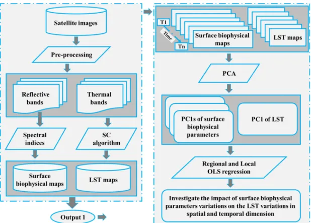
The methodology shown in Figure3presents a spatiotemporal integrated model for characterizing the impact of the surface biophysical parameters variations on LST variations. Firstly, the utilized satellite images were preprocessed (atmospheric corrections, radiometric corrections, restoring the values of missed pixels for scan line corrector (SLC)-off images, and a subset of the study area).
Secondly, the LST and various surface biophysical parameters were extracted based on reflective and thermal bands of Landsat imagery, MODIS product, and meteorological data for the period from 1985 to 2018. Thirdly, the principal component analysis (PCA) technique was employed to determine the degree of variation of the LST and surface biophysical parameters in the temporal dimension at the pixel scale. Fourthly, the impact of the surface biophysical parameters variations on LST variations was assessed by investigating the relationship between the first principal components (PC1s) of LST and each surface biophysical parameter at the regional and pixel scales by using ordinary least squares (OLS) regression. Finally, the relationship between the LST PC1s and effective surface biophysical parameters was analyzed using multivariate OLS regression with regional and local approaches.
Remote Sens. 2019, 11, x FOR PEER REVIEW 5 of 23
3.2. Methods
The methodology shown in Figure 3 presents a spatiotemporal integrated model for characterizing the impact of the surface biophysical parameters variations on LST variations. Firstly, the utilized satellite images were preprocessed (atmospheric corrections, radiometric corrections, restoring the values of missed pixels for scan line corrector (SLC)‐off images, and a subset of the study area). Secondly, the LST and various surface biophysical parameters were extracted based on reflective and thermal bands of Landsat imagery, MODIS product, and meteorological data for the period from 1985 to 2018. Thirdly, the principal component analysis (PCA) technique was employed to determine the degree of variation of the LST and surface biophysical parameters in the temporal dimension at the pixel scale. Fourthly, the impact of the surface biophysical parameters variations on LST variations was assessed by investigating the relationship between the first principal components (PC1s) of LST and each surface biophysical parameter at the regional and pixel scales by using ordinary least squares (OLS) regression. Finally, the relationship between the LST PC1s and effective surface biophysical parameters was analyzed using multivariate OLS regression with regional and local approaches.
Figure 3. The flowchart of the analytical procedures.
3.2.1. Image Preprocessing
In this study, the fast line‐of‐sight atmospheric analysis of hypercubes (FLAASH) model was used for atmospheric correction. This module uses the atmospheric radiative transfer (MODTRAN6) model for the atmospheric correction. To run FLAASH, some parameters, including satellite overpass time, sensor altitude, geographical location, specific atmospheric model related to the region, and solar zenith angle, are considered [55]. The equations presented by Chander et al. and Mishra et al.
[56,57] were used for the radiometric calibration of the satellite images acquired by Landsat 5, 7, and 8. The data obtained from the USGS website included the highest quality Level‐1 Precision Terrain (L1TP) data, which are appropriate for time series analysis. Landsat imagery was geo‐referenced with the root mean square error less than a half pixel [19,58].
Figure 3.The flowchart of the analytical procedures.
3.2.1. Image Preprocessing
In this study, the fast line-of-sight atmospheric analysis of hypercubes (FLAASH) model was used for atmospheric correction. This module uses the atmospheric radiative transfer (MODTRAN6) model for the atmospheric correction. To run FLAASH, some parameters, including satellite overpass time, sensor altitude, geographical location, specific atmospheric model related to the region, and solar zenith angle, are considered [55]. The equations presented by Chander et al. and Mishra et al. [56,57] were used for the radiometric calibration of the satellite images acquired by Landsat 5, 7, and 8. The data obtained from the USGS website included the highest quality Level-1 Precision Terrain (L1TP) data, which are appropriate for time series analysis. Landsat imagery was geo-referenced with the root mean square error less than a half pixel [19,58].
Remote Sens.2019,11, 2094 6 of 22
Landsat 7 ETM+has been suffering from an instrument failure since year 2003, and reducing pixel capturing by approximately 22% per scene [59]. In this study, in order to address the unscanned line issue, the neighborhood similar pixel interpolator (NSPI) method developed by Chen et al. was used to fill the gaps in the SLC-offin Landsat 7 ETM+images [60]. In order to interpolate the pixel values within unscanned lines, the NSPI method assumed that the same-class neighboring pixels around the un-scanned pixels have similar spectral characteristics, and that these neighboring and un-scanned pixels exhibit similar patterns of spectral differences for each date. It has been documented that the method can restore values of missed pixels very accurately, especially well in heterogeneous regions [60].
3.2.2. LST and Surface Biophysical Parameters
LST was calculated from Landsat 5, 7, and 8 by using the single channel (SC) [61,62] algorithm based on Equation (1). Since the thermal band 11 of Landsat 8 has a bias and a large error in calculating the LST [63], band 10 of the Landsat 8 imagery was used to calculate the LST through the SC algorithm.
LST = γ 1
ε(ψ1Lλ+ψ2)+ψ3
+δ, (1)
where LST is the land surface temperature (Kelvin), Lλis the spectral radiance at the sensor in terms of Watts/(m2sr um) in the thermal band,ε is land surface emissivity (LSE), andγandδare two parameters dependent on the Plank function (see [62,64]). The variables ofψ1,ψ2, andψ3are constant atmospheric functions [61,62]. The LSE for each date were retrieved by the NDVI threshold method (NDVITHM) [62,65].
In this study, thermal bands of Landsat 5 and 8 were resampled to 30 m with the cubic method.
Then, based on Landsat imagery by combining resampled thermal bands with an LSE with a spatial resolution of 30 m, the LST with a spatial resolution of 30 m was obtained.
The accuracy of LST values was evaluated using MOD11A1 and soil temperature data recorded by ground-based devices at the moment of the satellite’s overpass. The correlation coefficient and root mean square error (RMSE) were calculated between the LST values obtained from the Landsat images and the soil temperature measured at location of the meteorological station. In addition, the values of the correlation coefficient and RMSE were calculated between the mean LST obtained from the Landsat image and MOD11A1 of the case study for the years 2001 to 2018.
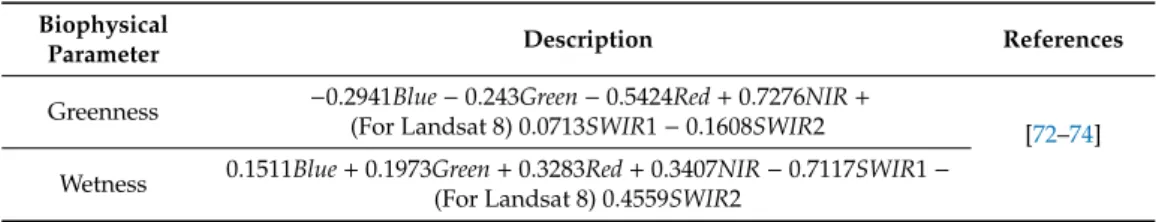
To assess the impact of each biophysical parameter changes on the LST variations, various spectral indices were computed to extract the surface biophysical parameters based on Landsat 5, 7, and 8 imagery. In this study, NDVI [66], the soil-adjusted vegetation index (SAVI) [67], normalized difference water index (NDWI) [68], NDBI [69], albedo [70,71], and tasseled cap transformation (TCT) components, including brightness, greenness, and wetness [72–74], were used to represent the surface biophysical parameters (Table1).
Table 1.Description of surface biophysical parameters.
Biophysical
Parameter Description References
NDVI ρρNIR−ρRed
NIR+ρRed [66]
SAVI (1+L)(ρ ρNIR−ρRed)
NIR+ρRed+L [67]
NDWI ρρGREEN−ρNIR
GREEN+ρNIR [68]
NDBI ρρSWIRSWIR+−ρρNIRNIR [69]
Brightness 0.3029Blue+0.2786Green+0.4733Red+0.5599NIR+0.5080SWIR1+
(For Landsat 8) 0.1872SWIR2 [72–74]
Remote Sens.2019,11, 2094 7 of 22
Table 1.Cont.
Biophysical
Parameter Description References
Greenness −0.2941Blue−0.243Green−0.5424Red+0.7276NIR+
(For Landsat 8) 0.0713SWIR1−0.1608SWIR2 [72–74]
Wetness 0.1511Blue+0.1973Green+0.3283Red+0.3407NIR−0.7117SWIR1− (For Landsat 8) 0.4559SWIR2
3.2.3. LST and Surface Biophysical Parameters Variations
PCA is one of the techniques for determining variations of environmental parameters in the temporal dimension [75–77]. The variations of environmental parameters in the temporal dimension can be examined on a pixel scale using PCA [78–80]. To model the variations of each particular parameter over a given time interval, a PCA model was applied to its specific values over a time scale at the pixel scale. If there arenimages during each specific interval, for each pixel,nvalues of each surface biophysical parameters and LST were modeled. As a result, for modeling the variation of each parameter, the PCA model was implemented onnvalues of each pixel [79]. The PC1 output can contain both negative and positive values. A higher and more positive value of a pixel in PC1 indicates that the values of this pixel have been large and unchanged over time. In contrast, a lower and more negative value of a pixel in PC1 indicates that the values of that pixel have been low and unchanged over time. A PC1 value close to zero indicates that changes in the values of the pixel have been high over time [78–80].
Due to the limited size and flatness of the study area, we assumed that the impact of the climatic and topographic parameters on LST spatial distribution remained the same and that the spatial variations in LST were mainly associated with the changes in surface biophysical parameters such as brightness, greenness, and wetness of surface. The climate background difference can only affect the absolute LST values but not affect the distribution pattern of the LST in one date. However, it is difficult to compare directly the impact of the surface biophysical parameters on LST due to the climate background difference in the temporal dimension. To solve this problem, a normalization technique was used. Therefore, normalization to the LST and surface biophysical parameters with different climate backgrounds can rescale each parameter to the same level between 0 and 1 and thus reduce the climate background difference [8,19,81]. By utilizing minima and maxima for each parameter, all LST and surface biophysical parameters maps were normalized using Equation (2) [81]:
NParameteri= Parameteri−Parametermin Parametermax−Parametermin
(2) where NParameteriis the normalized LST and surface biophysical parameters of i pixel, Parameteri
the LST and surface biophysical parameters of i pixel, Parameterminthe minimum, and Parametermax
the maximum LST and surface biophysical parameters value in each date. In this study, a PCA model was applied on normalized LST and surface biophysical parameters.
On the other hand, PC1 contains the major information of variability in the time series, whereas the other PCs contain the seasonal variability of the time series, each related to a certain parameter or parameters [46–48].
3.2.4. Impact of Surface Biophysical Parameter Variations on LST Variations
To investigate the impact of the surface biophysical parameters variations on LST variations in both spatial and temporal dimensions, the combination of PCA [82] and OLS regression [83] was employed. In this step, to analyze the impact of variations in the surface biophysical parameters on the LST variations in the temporal and spatial dimensions in an integrated manner, the relationship between the PC1 of the LST and PC1 of each surface biophysical parameter was examined using the OLS regression with regional and local optimization. The correlation coefficient and RMSE were used
Remote Sens.2019,11, 2094 8 of 22
to determine the amount of the impact. The higher correlation coefficient values and lower RMSE indicate the greater impact of changing a particular parameter on the LST variation. To determine the spatial distribution of the most influential biophysical parameter on the LST variations in the study area, the RMSE value between the observed and modeled LST variations based on each biophysical parameter variations was compared.
Regional and Local Optimization
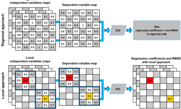
In this study, two different approaches of regional and local optimization were applied to solve the regression coefficients of the OLS regression in analyzing the impact of different surface biophysical parameters changes on the LST variations. In the regional optimization, the values of all pixels (the whole region) of the dependent variable (PC1 of LST) and independent variables (PC1s of biophysical parameters) were used in OLS regression. Furthermore, the local optimization approach was utilized for analyzing the impact of different surface biophysical parameters changes on the LST variations. In the local optimization, the regression coefficients of the surface biophysical parameters were calculated for each pixel individually. In order to determine the optimal value of the regression coefficient associated with each biophysical parameter for each pixel, only the values of neighboring pixels in the spatial window were introduced in OLS regression. OLS regression with a moving window provided the optimal values of the regression coefficients on the pixel scale. In this approach we used all the pixels in the window to get the optimal value of the regression coefficient for the center pixel.
The conceptual model of regional and local approaches to calculate the optimal values of the regression coefficients is shown in Figure4.
Remote Sens. 2019, 11, x FOR PEER REVIEW 8 of 23
Regional and Local Optimization
In this study, two different approaches of regional and local optimization were applied to solve the regression coefficients of the OLS regression in analyzing the impact of different surface biophysical parameters changes on the LST variations. In the regional optimization, the values of all pixels (the whole region) of the dependent variable (PC1 of LST) and independent variables (PC1s of biophysical parameters) were used in OLS regression. Furthermore, the local optimization approach was utilized for analyzing the impact of different surface biophysical parameters changes on the LST variations. In the local optimization, the regression coefficients of the surface biophysical parameters were calculated for each pixel individually. In order to determine the optimal value of the regression coefficient associated with each biophysical parameter for each pixel, only the values of neighboring pixels in the spatial window were introduced in OLS regression. OLS regression with a moving window provided the optimal values of the regression coefficients on the pixel scale. In this approach we used all the pixels in the window to get the optimal value of the regression coefficient for the center pixel. The conceptual model of regional and local approaches to calculate the optimal values of the regression coefficients is shown in Figure 4.
Figure 4. Conceptual model for determining regression coefficients with regional and local optimization.
The moving window size (MWS) is also directly related to the accuracy of LST variation modeling. The criteria for selecting the appropriate MWS according to the homogeneity degree of surface biophysical parameters in study area should be determined. In this study, the semivariance function was used for determining the appropriate MWS. See detail of this function in [84]. The optimal MWS for this study area yielded 21 × 21 pixels.
3.2.5. Modeled LST Variations Based on Multivariate OLS Regression
In this study, through the simultaneous consideration of PC1 of the most influential biophysical parameter, the LST variations was modeled. For this purpose, the multivariate OLS regression with both regional and local optimization was employed. In this study, from each group of indices related to impervious surfaces (albedo, NDBI, and brightness obtained from tasseled cap), vegetation covers (NDVI, SAVI, and greenness obtained from Tasseled cap), and wetness surfaces (NDWI and wetness obtained from tasseled cap), one parameter was selected as the most effective parameter for modeling
Figure 4.Conceptual model for determining regression coefficients with regional and local optimization.
The moving window size (MWS) is also directly related to the accuracy of LST variation modeling.
The criteria for selecting the appropriate MWS according to the homogeneity degree of surface biophysical parameters in study area should be determined. In this study, the semivariance function was used for determining the appropriate MWS. See detail of this function in [84]. The optimal MWS for this study area yielded 21×21 pixels.
Remote Sens.2019,11, 2094 9 of 22
3.2.5. Modeled LST Variations Based on Multivariate OLS Regression
In this study, through the simultaneous consideration of PC1 of the most influential biophysical parameter, the LST variations was modeled. For this purpose, the multivariate OLS regression with both regional and local optimization was employed. In this study, from each group of indices related to impervious surfaces (albedo, NDBI, and brightness obtained from tasseled cap), vegetation covers (NDVI, SAVI, and greenness obtained from Tasseled cap), and wetness surfaces (NDWI and wetness obtained from tasseled cap), one parameter was selected as the most effective parameter for modeling LST variations. Finally, for accuracy assessment, the correlation coefficient and RMSE between the observed and modeled values of LST variations at regional and local optimization were investigated.
4. Results
4.1. LST and Surface Biophysical Parameters
The correlation coefficient yielded 0.91 between Landsat-derived LST values and soil temperatures measured at the location of the meteorological station. Furthermore, the correlation coefficient between the mean LST obtained from Landsat and that from MOD11A1 reached 0.93. These results indicate that LST calculated with the Landsat images possessed a high accuracy. The RMSE parameter yielded 1.80◦C between the Landsat LSTs and the soil temperatures, and 1.37◦C between the mean LST from Landsat images and MOD11A1. According to previous studies [19,85,86], RMSE value of less than 2◦C between the mean LST obtained from Landsat and MOD11A1 indicates the high accuracy of LST derivation. Examples of the derived LST maps at different days from 1985 to 2018 are shown in Figure5. The results indicated that LST values increased over the years of studied period.
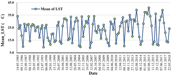
The mean LST of the region was further investigated from 1985 to 2018 and the results are shown in Figure6. The result indicates that the mean LST for the study area changed over the time.
The maximum of the mean LST in the warm months (May and June) in the late 1980s and early 1990s was around 25◦C, with a significant increase to over 30◦C after 2010. Less variations occurred in the minimum of the mean LST in the cold months (approximately 2◦C).
The mean normalized values of each surface biophysical parameter during 1985–2018 are shown in Figure7.
According to Figure7, the mean normalized values for the surface biophysical parameters varied significantly in the period of 1985–2018. The standard deviation of the mean values of the NDVI, NDBI, NDWI, greenness, wetness, albedo, SAVI, and brightness are 0.0718, 0.086, 0.074, 0.115, 0.075, 0.1135, 0.067, and 0.098, respectively. The correlation coefficient between the observed mean values of the normalized LST (NLST) and mean normalized values of the surface biophysical parameters are shown in Table2.
Table 2.Correlation coefficient between the mean values of the NLST and mean normalized values of surface biophysical parameters.
Surface Biophysical
Parameters
NDVI NDBI NDWI Albedo Greenness Wetness Brightness SAVI
R squared −0.44 0.71 0.29 0.58 −0.57 −0.68 0.63 −0.46
p-Value 0.01 0.01 0.02 0.01 0.00 0.01 0.02 0.00
The results of the initial investigation indicate that NDWI and NDBI have the lowest and the highest impact on the LST, respectively. The correlation coefficient between the LST and NDBI was high [36].
Remote Sens.2019,11, 2094 10 of 22
Remote Sens. 2019, 11, x FOR PEER REVIEW 10 of 23
14/05/1985 07/06/1988 18/05/1998
12/08/2003 19/05/2007 24/11/2009
27/03/2011 25/07/2014 18/06/2015
23/08/2016 10/08/2017 22/03/2018
Figure 5. Examples of land surface temperature (LST) maps (°C) for the time period of 1985–2018 in Babol City, Iran.
Figure 5.Examples of land surface temperature (LST) maps (◦C) for the time period of 1985–2018 in Babol City, Iran.
Remote Sens.2019,11, 2094 11 of 22
Remote Sens. 2019, 11, x FOR PEER REVIEW 11 of 23
Figure 6. The mean LST in Babol, Iran, from 1985 to 2018 (°C).
5.0 15.0 25.0 35.0 45.0
14.05.1985 09.11.1986 25.09.1987 08.12.1988 28.05.1990 18.06.1992 23.07.1993 06.08.1998 29.01.1999 15.12.1999 26.07.2000 16.04.2001 14.08.2001 12.08.2003 26.05.2004 20.12.2004 21.11.2005 19.07.2006 12.02.2007 26.10.2007 04.10.2008 27.07.2009 24.11.2009 04.06.2010 19.09.2010 12.04.2011 08.12.2011 08.11.2012 27.11.2013 02.08.2014 08.12.2014 01.05.2015 05.08.2015 11.12.2015 29.12.2016 07.06.2017 14.11.2017 22.03.2018
Mean_LST ( C)
Date Mean of LST
0.40 0.60 0.80
NDVI
0.20 0.40 0.60 0.80
NDBI
0.20 0.40 0.60
NDWI
0.20 0.40 0.60 0.80
Greenness
0.40 0.60 0.80 1.00
Wetness
Figure 6.The mean LST in Babol, Iran, from 1985 to 2018 (◦C).
Remote Sens. 2019, 11, x FOR PEER REVIEW 11 of 23
Figure 6. The mean LST in Babol, Iran, from 1985 to 2018 (°C).
5.0 15.0 25.0 35.0 45.0
14.05.1985 09.11.1986 25.09.1987 08.12.1988 28.05.1990 18.06.1992 23.07.1993 06.08.1998 29.01.1999 15.12.1999 26.07.2000 16.04.2001 14.08.2001 12.08.2003 26.05.2004 20.12.2004 21.11.2005 19.07.2006 12.02.2007 26.10.2007 04.10.2008 27.07.2009 24.11.2009 04.06.2010 19.09.2010 12.04.2011 08.12.2011 08.11.2012 27.11.2013 02.08.2014 08.12.2014 01.05.2015 05.08.2015 11.12.2015 29.12.2016 07.06.2017 14.11.2017 22.03.2018
Mean_LST ( C)
Date Mean of LST
0.40 0.60 0.80
NDVI
0.20 0.40 0.60 0.80
NDBI
0.20 0.40 0.60
NDWI
0.20 0.40 0.60 0.80
Greenness
0.40 0.60 0.80 1.00
Wetness
Figure 7.Cont.
Remote Sens.2019,11, 2094 12 of 22
Remote Sens. 2019, 11, x FOR PEER REVIEW 12 of 23
Figure 7. The mean normalized values of each surface biophysical parameter.
4.2. LST and Surface Biophysical Parameters Variations
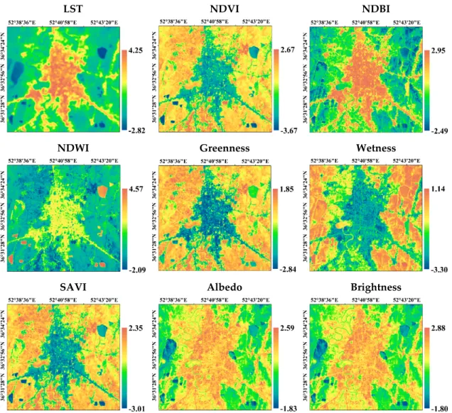
The PC1 maps for the LST and other surface biophysical parameters are shown in Figure 8. A higher and more positive value of a pixel in PC1 indicates that the values of this pixel have been large and unchanged over time (red regions in Figure 8). In contrast, a lower and more negative value of a pixel in PC1 indicates that the values of that pixel have been low and unchanged over time (blue regions in Figure 8). A PC1 value close to zero indicates that changes in the values of pixels have been high over time.
Based on Figure 8, the pixels that had been built‐up lands in most of the dates had the highest values of LST, NDBI, albedo, and brightness and, therefore, the highest PC1s of LST, NDBI, albedo, and brightness values. This is in contrast to those pixels that had low values of NDVI, SAVI, and greenness, and thus lower values of the PCIs for these surface parameters. The pixels that changed from green space and agriculture lands to built‐up land, had PC1 values of LST and surface biophysical parameters close to zero.
0.00 0.20 0.40 0.60
Albedo
0.20 0.40 0.60
SAVI
0.00 0.20 0.40 0.60
14.05.1985 09.11.1986 25.09.1987 08.12.1988 28.05.1990 18.06.1992 23.07.1993 06.08.1998 29.01.1999 15.12.1999 26.07.2000 16.04.2001 14.08.2001 12.08.2003 26.05.2004 20.12.2004 21.11.2005 19.07.2006 12.02.2007 26.10.2007 04.10.2008 27.07.2009 24.11.2009 04.06.2010 19.09.2010 12.04.2011 08.12.2011 08.11.2012 27.11.2013 02.08.2014 08.12.2014 01.05.2015 05.08.2015 11.12.2015 29.12.2016 07.06.2017 14.11.2017 22.03.2018
Brightness
Figure 7.The mean normalized values of each surface biophysical parameter.
4.2. LST and Surface Biophysical Parameters Variations
The PC1 maps for the LST and other surface biophysical parameters are shown in Figure8.
A higher and more positive value of a pixel in PC1 indicates that the values of this pixel have been large and unchanged over time (red regions in Figure8). In contrast, a lower and more negative value of a pixel in PC1 indicates that the values of that pixel have been low and unchanged over time (blue regions in Figure8). A PC1 value close to zero indicates that changes in the values of pixels have been high over time.
Based on Figure8, the pixels that had been built-up lands in most of the dates had the highest values of LST, NDBI, albedo, and brightness and, therefore, the highest PC1s of LST, NDBI, albedo, and brightness values. This is in contrast to those pixels that had low values of NDVI, SAVI, and greenness, and thus lower values of the PCIs for these surface parameters. The pixels that changed from green space and agriculture lands to built-up land, had PC1 values of LST and surface biophysical parameters close to zero.
4.3. Impact of Surface Biophysical Parameters Variations on LST Variations 4.3.1. Regional Optimization
The results of the relationship between the PC1 of LST and the PC1 of each surface biophysical parameters based on OLS regression with regional optimization are presented in Figure9.
Figure9indicates that among the spectral indices considered, the variations in the greenness from TCT components (from group of biophysical parameters related to vegetation covers), NDBI (from group of biophysical parameters related to impervious surfaces), and wetness from TCT components (from group of biophysical parameters related to wetness surfaces) have the highest impact on the LST variations, respectively. Based on regional optimization, among the various surface biophysical parameters, NDBI variations had the highest impact on the LST variations. The results of the initial
Remote Sens.2019,11, 2094 13 of 22
investigation indicate that in this study area, variations of NDWI and NDBI have the lowest and the highest impact on the LST variations, respectively (Figure9). The correlation coefficient between the LST and NDBI was high [36].Remote Sens. 2019, 11, x FOR PEER REVIEW 13 of 23
LST NDVI NDBI
NDWI Greenness Wetness
SAVI Albedo Brightness
Figure 8. PC1 maps of LST and various surface biophysical parameters.
4.3. Impact of Surface Biophysical Parameters Variations on LST Variations
4.3.1. Regional Optimization
The results of the relationship between the PC1 of LST and the PC1 of each surface biophysical parameters based on OLS regression with regional optimization are presented in Figure 9.
Figure 9 indicates that among the spectral indices considered, the variations in the greenness from TCT components (from group of biophysical parameters related to vegetation covers), NDBI (from group of biophysical parameters related to impervious surfaces), and wetness from TCT components (from group of biophysical parameters related to wetness surfaces) have the highest impact on the LST variations, respectively. Based on regional optimization, among the various surface biophysical parameters, NDBI variations had the highest impact on the LST variations. The results of the initial investigation indicate that in this study area, variations of NDWI and NDBI have the lowest and the highest impact on the LST variations, respectively (Figure 9). The correlation coefficient between the LST and NDBI was high [36].
Figure 8.PC1 maps of LST and various surface biophysical parameters.
4.3.2. Local Optimization
The results of the correlation coefficient and RMSE between the observed and modeled values of the LST variations based on the spatial moving window method are shown in Figure10and Table3.
The results indicated the values of the correlation coefficient and RMSE between the observed and modeled values of LST variations are variable spatially.
Table 3.Mean and standard deviation of the correlation coefficient and RMSE between the observed and modeled values of the LST variations at the pixel scale based on the variations of each surface biophysical parameters.
Surface Biophysical
Parameters NDVI NDBI NDWI Albedo Greenness Wetness Brightness SAVI Mean value of R −0.37 0.75 0.29 0.59 −0.44 −0.70 0.65 −0.37
Std of R 0.50 0.22 0.54 0.30 0.48 0.25 0.26 0.30
Mean value of RMSE 1.15 0.71 1.17 1.05 1.06 1.03 1.05 1.15
Std of RMSE 0.95 0.32 0.95 0.48 0.77 0.87 0.49 0.91
Remote Sens.2019,11, 2094 14 of 22
The results of Table3indicate that among the spectral indices considered for the surface biophysical parameters of the vegetation cover, impervious surface cover, and wetness surface cover, the variation in the greenness (from the group of biophysical parameters related to vegetation covers), NDBI (from the group of biophysical parameters related to impervious surfaces), and wetness (from the group of biophysical parameters related to wetness surfaces) have the highest effect on the LST variations, respectively. Based on the RMSE between the observed and modeled values of LST variations at the pixel scale for greenness, NDBI, and wetness variations (Figure10), the results of the spatial distribution of the most effective biophysical parameter variations on LST variations are shown in Figure11.
Remote Sens. 2019, 11, x FOR PEER REVIEW 14 of 23
Figure 9. Relationship between the PC1 of LST and the PC1 of each surface biophysical parameters using OLS regression with a regional approach.
4.3.2. Local Optimization
The results of the correlation coefficient and RMSE between the observed and modeled values of the LST variations based on the spatial moving window method are shown in Figure 10 and Table 3. The results indicated the values of the correlation coefficient and RMSE between the observed and modeled values of LST variations are variable spatially.
Table 3. Mean and standard deviation of the correlation coefficient and RMSE between the observed and modeled values of the LST variations at the pixel scale based on the variations of each surface biophysical parameters.
Surface Biophysical
Parameters NDVI NDBI NDWI Albedo Greenness Wetness Brightness SAVI Mean value of R −0.37 0.75 0.29 0.59 −0.44 −0.70 0.65 −0.37 Std of R 0.50 0.22 0.54 0.30 0.48 0.25 0.26 0.30 Mean value of RMSE 1.15 0.71 1.17 1.05 1.06 1.03 1.05 1.15 Std of RMSE 0.95 0.32 0.95 0.48 0.77 0.87 0.49 0.91 Figure 9.Relationship between the PC1 of LST and the PC1 of each surface biophysical parameters using OLS regression with a regional approach.
The results show that variations of NDBI, wetness, and greenness from TCT were the most influential parameters on LST variations, accounting for 43%, 38%, and 19% of the LST variations, respectively. The greenness variation had a lower impact on the LST variations than NDBI and wetness.
4.4. Modeled LST Variations Based on Multivariate OLS Regression
Modeled LST variations based on NDBI, greenness, and wetness variations using multivariate OLS regression with regional and local optimizations are shown in Figure12.
Remote Sens.2019,11, 2094 15 of 22
Remote Sens. 2019, 11, x FOR PEER REVIEW 15 of 23
R squared RMSE R squared RMSE
NDVI
NDBI
NDWI
Albedo
Greenness
Wetness
Brightness
SAVI
Figure 10. Correlation coefficient and RMSE between the observed and modeled values of LST variations at the pixel scale based on each surface biophysical parameter variations.
Figure 10. Correlation coefficient and RMSE between the observed and modeled values of LST variations at the pixel scale based on each surface biophysical parameter variations.