Photometer Long-Term Measurements in Ny-Ålesund
Master Thesis
Sandra Karen Graßl
April 3, 2019
Supervisors:
Prof. Dr. Bernhard Mayer Ludwig-Maximilians University Munich
Faculty of Physics Meteorology
Dr. Christoph Ritter
Alfred Wegener Institute, Helmholtz Centre for polar and marine research, Potsdam Section Physics of the Atmosphere
anhand von Langzeit-Photometerdaten in Ny-Ålesund
Masterarbeit
Sandra Karen Graßl
April 3, 2019
Betreuer:
Prof. Dr. Bernhard Mayer
Ludwig-Maximilians Universität München Fakultät für Physik
Meteorologie
Dr. Christoph Ritter
Alfred-Wegener-Institut, Helmholtz-Zentrum für Polar- und Meeresforschung, Potsdam Sektion Physik der Atmosphäre
On the base of sun and star photometer measurements located at the German-French polar research base in Ny-Ålesund (78.923◦N, 11.928◦E), Svalbard, long-term changes (2001-2017 with focus on 2009-2017) of aerosol properties in the European Arctic are analysed. The main focus were physical aerosol properties like aerosol optical depth (AOD) or Ångström exponent, during the Arctic Haze season in spring compared to summer months. The presence of polar night and day is the limitating factor of available photometer measurement data. To get a full year-round data set a star photometer was also taken into account for the time between October and March.
In order to gain more information out of the measurement data of the photometers and to reduce the error of fitting the data to the Ångström law a new ansatz is also discussed in this thesis. With the radiative transfer calculator libRadtran artificial aerosol distributions were created to analyse the information content of real (noisy) photometer data. Indeed it was found that the new ansatz with wavelength dependent Ångström exponent reveals valuable information about the Arctic aerosol.
Monthly means of the measured AOD of the years 2009-2017 are compared with monthly means of previous studies to see changes in the properties of aerosol. Additionally, a comparison of sun and star photometer at the same site and the same years is also done.
Because photometer data has no height information a comparison with the Lidar is presented.
To study possible sources and sinks of aerosol, 5-days back-trajectories were calculated with the FLEXTRA model at three different arriving heights (500m,1000m and1500m) at 12 UTC over Zeppelin Station, at Zeppelin mountain474m above sea level and close to the village Ny- Ålesund.
Beside of the pathway of the aerosol into the European Arctic based on the calculated back- trajectories the influence of the lowermost100hP aatmospheric layer is also analysed. Especially aerosol is highly affected by cloud formation and is removed out of the atmosphere by precipi- tation, areas with a high probability of cloud formation is also taken into account.
1. Introduction 7
2. Theory on tropospheric aerosol 9
2.1. Sources and sinks . . . 10
2.2. Interaction of aerosols and molecules with radiation . . . 12
2.3. Aerosol Optical Depth . . . 13
2.4. Impact of aerosols on polar climate . . . 15
3. Data Processing and Methods 18 3.1. Instruments . . . 18
3.1.1. Raman Lidar "KARL" . . . 18
3.1.2. Sun Photometer . . . 19
3.1.3. Star Photometer . . . 20
3.2. Data fitting and processing . . . 26
3.3. Mie Calculus . . . 35
3.4. Case study . . . 41
3.5. Error Estimation . . . 43
3.6. Back-trajectory analysis . . . 44
4. Results 47 4.1. Trends in the AOD . . . 47
4.1.1. Polar day . . . 47
4.1.2. Polar night . . . 50
4.2. Comparison of sun and star photometer . . . 52
4.3. Trend of AOD over the whole year . . . 54
4.4. Comparison with previous measurements . . . 54
4.5. Aerosol load during polar night . . . 55
4.6. Changes of heat transfer from mid latitudes . . . 55
4.7. Aerosol load and properties . . . 57
4.8. FLEXTRA back-trajectories . . . 59
4.8.1. Aerosol origin due to arriving air pollution . . . 60
4.8.2. Aerosol sources and sinks . . . 62
4.8.3. Remarks on the advection altitude . . . 64
5. Conclusion 68
6. Outlook 69
7. Danksagung 76
A. Appendix 77
B. Abbreviations 86
1. Introduction
Figure 1: Location of Ny-Ålesund in Svalbard (source: https:
//toposvalbard.npolar.no/
While technology in every part of life is becoming better and better, the hu- manity changes all ecosystems on Earth and also the atmosphere. Due to these changes both the weather and the climate change, especially in the Arctic. When both poles change their actual habit, it will influence also the life of people liv- ing in the mid-latitudes. The Arctic as a whole ecosystem can be seen as an early warning system for anthropogenic ef- fects on the global climate. Especially here the impact is visible due to rapid decreases of glaciers and sea ice as well as an increasing active layer of the per- mafrost. The impact of increasing tem- perature is such large and reinforces itself, that it is known as Arctic Amplification (Pi- than and Mauritsen, 2014). That’s why lots of research is done at very remote places in high latitudes, like in Ny-Ålesund, a small research village in north-west of Sval- bard.
As time goes by more and more fossil fuel is required to deal with the global need of energy for transport, industry and heating.
Most of the aerosol is emitted on the ground and mostly exuded into the lowermost 10 km of the atmosphere, the so-called troposphere. Also in this part of the atmosphere the weather takes place. Because water droplets can not be formed with a typical saturation in the atmosphere, aerosols as starting cores for droplets are needed. Due to the changes of releasing aerosols in air, cloud formation itself and their probability of appearance change because more condensation nuclei are available in the atmosphere. With the changes of cloud appearance the radiation to the Earth’s surface is effected as well. While solar shortwave radiation is scattered into space, the thermal radiation, emitted by the Earth itself, is back-scattered to the ground again which leads to a temperature increase there.
A main challenge for climate modeling are aerosols because they can have a cooling as well as a warming effect for the surface depending on its albedo. The ocean has a quite low albedo.
When clouds, which have a much higher albedo, cover the sea, the albedo rises and the back into space scattered solar radiation as well. On the other hand, when black carbon is deposited over ice or snow it absorbs more energy, the ice melts and the ground starts to warm up.
When the ice starts to melt more and more each year, more and more energy is deposited to Earth and the effect becomes stronger and stronger. Especially in the Arctic this is a major
problem and is measured in winter times with a temperature increase of 3K per decade (Ma- turilli and Kayser, 2017).
Continuously the whole Earth is monitored by ground and space born instruments detecting global changes on short terms. But due to extreme conditions the Arctic is really hard to cover, even with satellites. For space-born observations it is hard to determine between ice, snow and clouds because the contrast is very low. Flying on polar orbits costs much more energy, which reduces the life-time of them. Additionally, lots of instruments have problems with the high albedo of the snow (Curry et al., 1996) and ice or need direct solar radiation for measurements, like measuring the total ozone concentration in a vertical column. During polar night these instruments can not operate and one has to take ground-based data of only a few polar research stations in the Arctic. Therefore, it is even a bigger challenge to interpret the few available data correctly.
Every spring (March, April) the so-called Arctic Haze is observed in the Arctic (Quinn et al., 2007). It dramatically reduces the visibility whereas the aerosol concentration on the other hand rises significantly during that time compared to summer months. In the dark season the aerosol sinks are reduced due to a larger snow and ice cover. Thus, the boundary layer is thermodynamically stably stratified, which leads to a smaller vertical atmospheric mixing.
Also the relative humidity is very low and aerosols are not washed out. Both effects increase the life time of the particles in the air. With in-situ measurements Shaw (1995) and Eckhardt et al. (2003) showed that mainly anthropogenic pollutants, like soot or CO, accumulate and are transported into the Arctic.
When the snow is already gone, mostly small particles are observed (Engvall et al., 2008; Tunved et al., 2013). But it is not completely clear where this size of particles comes from.
To understand more about the polar atmosphere, especially the origin of the Arctic Haze, aerosol properties, their annual cycle and longterm changes of the atmosphere, the aerosol op- tical depth (AOD) is measured by sun photometers (summer) and a star photometer (winter) from 2001 to 2017 with the main focus on the years 2009 to 2017 because Stock (2010) has already done an evaluation of the sun photometer data from 1995 to 2008. As these instruments do not have a height information and the calibration of water vapor channels has very high uncertainties, Lidar (Light Detection and Ranging) and Radiosondes were also used. Apart from that the origin and the path of air masses arriving in the Arctic are investigated using 5-days back-trajectories.
All used instruments are obtained from Ny-Ålesund, a small research village at Kongsfjord in north-west of Svalbard at 78.923◦N, 11.928◦E.
2. Theory on tropospheric aerosol
The troposphere is the lowermost atmospheric layer, has a height of several kilometers (equator:
0-17 km, pole: 0-7 km) and concentrates around 80% of the total atmospheric mass. Beside the main two constituents, nitrogen (78%) and oxygen (21%), lots of trace gases and wafting solid or liquid particles like sea salt, black carbon, organic materials, desert dust or soil, form the atmosphere. All of these non gaseous constituents of the atmosphere are called aerosols.
A typical aerosol size distribution is shown in figure 2 with the classification of aerosols by Junge (1963) (table 1).
Declaration Size
Ultra-fine particle <0.01µm Aitken particle 0.01−0.1µm Accumulation particle 0.1−1µm Giant particle >1µm
Table 1: Size distribution of aerosols characterized by Junge (1963)
Figure 2: Particle size distribution for mid-latitude aerosol in abitrary units of concentration (Buseck and Schwartz, 2003)
Depending on their origin, aerosols and their trajectories through the atmosphere have dif- ferent and changing properties and chemical components because they are strongly affected by the surrounding atmosphere.
Most of the aerosols measured by in-situ measurements in Gruvebadet, Ny-Ålesund, are com- posed of the cations N a+, N H4 and the anions SO42− and Cl− (Udisti et al., 2016).
The interaction with light strongly depends on particle radii as they have to reach a certain radius of about 0.1µm to become visible for photometers. Usually photometers detect the two modes with the largest aerosol particles whereas they are called in literature "fine" and "coarse"
mode particles.
2.1. Sources and sinks
In general aerosols are classified in two categories depending on their primary origin, natural or anthropogenic. With the aid of vertical winds they are advected over thousands of kilometers.
Hence, lots of different types of aerosols can get into the Arctic within a few days (Park et al., 2017)
Anthropogenic aerosols, which reach the Arctic, are usually emitted as sulfates or black carbon by combustion processes in the mid-latitudes. Due to chemical reactions these particles contain mainly sodium with diameters of 0.2−2µm (Udisti et al., 2016).
Another kind of aerosols have a natural origin and therefore a great number of origins and enter the atmosphere as sea salt, pollen or dust due to mechanical forces, such as sea spray, volcanic eruption or erosion. Beside marine biogenic produced dimethyl sulfide, aerosols with natural origin are larger than anthropogenic ones and are characterised as giant particles within the Arctic Haze season (Quinn et al., 2007; Park et al., 2017). In summer the aerosol is smaller than in spring time (Udisti et al., 2016).
The other possible manifestation for aerosols are secundary ones which can be created via homogeneous or heterogeneous nucleation. By phase transition from gaseous to solid or liquid state new particles are created. This process is called homogeneous. Such gases are made by anthropogenic emission of sulfur compounds in exhaust gases of fuel as well as naturally containing dimethylsulphid or methane. These gas molecules have to accumulate via collisions of more than two slowly moving particles by Brownian motion. The new formed larger par- ticle saves most of the kinetic energy whereas two slower moving particles remain. In this case the kinetic energies of all involved particles are sufficiently small enough so that in the end gas molecules condensate and reach a critical radius to become stable. The probability for a collision of three particles is roughly proportional to the oversaturation of the molecules in the surrounding gas (Tunved et al., 2013). Because these new formed particles have only reached the critical radius they belong to the class of ultra-fine or Aitken particles. As time goes by molecules accumulate to the already existing ones and create larger particles.
When the particles are sufficiently large enough, the new formed particles are now called cloud condensation nuclei (CCN) and water condenses onto the surface because they support con- densation at supersaturation values (relative humidity > 100%) below the required size for homogeneous nucleation. For highly hygroscopic particles, like sodium chloride (N aCl) or am- monium sulfate ((N H4)2SO4) this effect is much more relevant. The resulting saturation vapor pressurees significantly decreases below the one of pure water becausees only depends on the absolute concentration of water molecules on the surface of the droplet. This leads to Raoult’s law:
e(T) = es(T)· nw
nw+nd (2.1)
Where e is the equilibrium vapour pressure over a solution with nw molecules of water and nd molecules of solute. es is the saturation vapour pressure with respect to a plane surface of water at the temperature of the system.
In theory it is also possible to create droplets only of pure water. But for this process a relative humidity of about 115% is required which is a very rare incident in nature.
This accumulation has a big impact on the chemical and physical properties of the original particles because chemical reactions can take place in the liquid phase. This process is called heterogeneous nucleation.
The lifetime of aerosols strongly depends on their size and chemical composition. Ultra-fine and Aitken particles have a much stronger motion than larger ones due to Brownian motion or diffusion. Because they move randomly, the probability of collisions with each other is very likely. This leads to larger particles with simultaneously decreasing particle number density.
The first very important sink is sedimentation or dry deposition. In this process aerosol finally hits obstacles, like buildings, trees or the ground, by Brownian motion and sticks to them.
Oriented motion induced by gradients or gravitation forces particles to sediment. The sedimen- tation velocity strongly depends on their size and density and is proportional to the squared radius of the particle. The larger aerosols become the more inert they get and do not follow streamlines of air as precisely as lighter ones. Therefore, they stick to obstacles more easily.
On the other hand accumulation mode particles with a diameter of around0.2µm(see table 2) are too large for Brownian motion but too light for self sedimentation by gravity. These kind of aerosols have the longest dwelling time. But the dwelling times are strongly affected by vertical wind motions.
ultra-fine Aitken accumulation giant aerosol diameter <0.02 µm 0.02−0.2 µm 0.2−2µm >2 µm
lower troposphere <1-24 h 6 d 8 d 1-7 d
upper troposphere <1-24 h 12 d 8 d 2-10 d
stratosphere <1-24 h 24 d 300 d <100 d
Table 2: Dwelling time of different types of aerosols in the atmosphere, classified by Junge (1963)
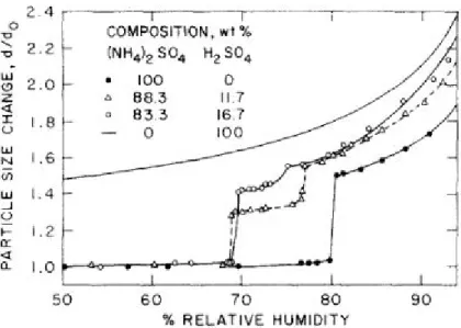
In contrast to the dry sedimentation aerosols also can be washed and rained out when they form clouds. This is called wet deposition after the hygroscopic growth of the aerosol already has taken place. Accumulation particles are the main sources for water droplets and cloud formation in case they have a hydrophilic chemical composition. At the so-called deliquescence point the relative humidity is sufficiently high enough to create a water shell around the aerosol which now has a solid core. How fast a particle grows is determined by its chemical composition and the quotient of its moist and dry diameter depending on the relative humidity around that particle. The more hydrophilic the core is the faster it grows and the larger it becomes. This quotient plotted over relative humidity leads to the typical hysteresis for this particular aerosol (figure 3). In case the aerosol comes out of a wet atmospheric layer and moves into a dry one,
the surrounding water shell remains up to a relative humidity of about70% for sulfates plotted in figure 3. Having a relative humidity smaller than this threshold the aerosol is not affected by water vapour. On the other side an aerosol particle coming out of a dry layer and being pushed into a wet one remains without liquid water shell up to a relative humidity of about 80%. This process is more important than the dry one because it directly affects the life-time of aerosols. Hence, the age of the air mass with the aerosol depends on the time of the last precipitation event.
Figure 3: Hysteresis of the hygroscopic growth of sulfuric acid and ammonium sulphate at25◦C (Tang et al., 1978)
2.2. Interaction of aerosols and molecules with radiation
Direct solar radiation measured at the ground is strongly affected by particles in the whole atmosphere via scattering, reflection, absorption, re-emission and extinction. The efficiency of all these processes depends on the incoming wavelength. The most important possibilities of interaction between aerosols and radiation are absorption and scattering.
Whereas absorption converges radiation into heat depending on wavelength and atmospheric constituents, scattering changes direction and intensity of the radiation. Elastic scattering takes place if energy and momentum of the photons are conserved before and after the scattering event. If due to light-matter interaction the particle is excited into a higher state and falls down to the initial state or a slightly higher one, the event is called inelastic scattering and is described as Raman scattering.
For a given wavelengthλ the scattering properties depend on size, shape and index of refrac- tion. In general no analytic solution can be found because the scattering is too complicated.
Only for special cases theories exist describing these scattering events. For spherical particles
Mie theory is used which is valid for arbitrary particle sizes. For small particles, compared to the wavelength of scattered light, Mie and Rayleigh theory become equal. As a consequence, scattering is described as Hertzian Dipole and classical electrodynamics.
Mie scattering
Mie scattering describes scattering of electromagnetic radiation on spherical particles. Only in case of spherical particles an analytical solution exists. In other cases the theory is analytically not closed.
This theory is valid for all sizes of spherical particles. Size parameter x = 2πrλ and complex index of refraction determine the spatial properties of the refracted light field. The photon gets mainly scattered in forward direction (Mie, 1908).
Rayleigh scattering
Rayleigh scattering is one limit of Mie scattering for small particles. It describes the interaction between tiny particles with a diameter much smaller than the wavelength and electromagnetic radiation. Particles may be individual atoms or molecules and have to have only a real part of an index of refraction with a value of about 1, which is more or less given for clear sky conditions and responsible for the blue colour of the sky.
Rayleigh scattering is a process of electric polarizability of the particles. Incoming radiation is an electromagnetic wave. The oscillating electric field of the radiation acts on the charges within a particle and forces them to move at the same frequency of the light. Therefore, Maxwell’s equations are simplified and the particle becomes a small radiating, Hertzian dipole which emits radiation. The scattering cross-section is proportional to λ−4. This leads to a very strong wavelength dependenet interaction between radiation and particles. The shorter the wavelengths are the larger the probability is the photon gets scattered at the particle.
Raman scattering
Raman scattering is the inelastic scattering of photons by molecules. When photons are scat- tered by atoms or molecules most of them are elastically Rayleigh scattered. So Raman scat- tering has also the λ−4 wavelength dependency. Only 1 out of 1000 photons is inelastically scattered by excitation. In the terrestrial atmosphere, most of the outgoing photons have a lower energy than the initial one. The easier an atom gets excited the higher the probabil- ity of such a scattering event becomes. This type of scattering becomes important for Lidar measurements.
2.3. Aerosol Optical Depth
The monochromatic extinction of the total vertical atmosphere α can always be written as the sum of the extinction coefficients of the Rayleigh scattering of air molecules αRay, the Mie scattering of aerosols αAer and absorptive contributions of some gases αGas like ozone, oxygen or water vapour:
α=aRay+aAer+aGas (2.2)
With equation 2.2 the total optical depthτext up to an heightH as the integral over the total atmospheric optical depth τ is defined as follows:
τext= Z H
0
a(z)dz
= Z H
0
[aRay(z) +aAer(z) +aGas(z)] dz
=τRay+τAer+τGas (2.3)
Using Lambert-Beer’s law aerosol optical depth (AOD) can be measured and computed.
Splitting the integral in three independent integrals is possible due to the assumption of only single scattering in the atmosphere. It is assumed that the intensity of direct solar radiation I0 decreases from top of the atmosphere to the ground depending on physical properties of the penetrated medium. The integral over possible types of extinction in the atmosphere of equation 2.3 can be simplified to three independent integrals in general because only direct solar radiation is considered. In case one photon is extincted by aerosol it can not be extincted anymore by another particle. Equation 2.4 shows the modified intensity decay for a ground based measurement.
I =I0·e−m·τext (2.4)
Here I is the radiation at the ground and m the penetrated air mass. Atmospheric refraction is also considered in this ansatz. In general m is defined as the length of the path through the atmosphere the light had to travel to reach the ground. The exact solution calculated in Kasten and Young (1989) can be simplified for a solar zenith angle θ >45◦:
m= 1
cosθ (2.5)
The refraction index of the atmosphere increases continuously coming from outer space be- cause the particle density increases exponentially in the same direction. Extraterrestrial radi- ation is refracted more and more the closer it gets to the ground because the refraction index n is proportional to the pressure p:
n = 77.6 T ·
p+4810·e T
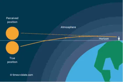
(2.6) Wherepis in milibars,T in Kelvin and eis expressed as the partial pressure of water vapuor in millibars. This leads to a curved path through the atmosphere. The closer the sun reaches the horizon the stronger the refraction takes place (figure 4).
To get a more precise result relative air masses for aerosol, Rayleigh atmosphere and ozone have to be calculated separately.
Using the formula by (Kasten, 1965) to receive the relative aerosol air mass:
mAer = 1
sin(hsun) + 0.0548·(hsun+ 2.65)−1.452 (2.7)
Figure 4: Changed apparent position of extraterrestrial objects due to atmospheric refraction (source: https://www.timeanddate.com/astronomy/refraction.html).
Wherehsun denotes the apparent solar elevation in degrees, which is always greater than the geometrical height of the sun due to a continuously changing refraction index of the atmosphere from top of atmosphere to the ground. To get hsun temperature as well as pressure profiles have to be known.
The relative Rayleigh air mass is calculated using (Kasten and Young, 1989):
mRay = 1
sin(hsun) + 0.50572·(hsun+ 6.07995)−1.6364 (2.8) The relative ozone air mass is calculated using WMO (2008):
mO3 = r+HO3
p(r+HO3)2−(rE +Hs)2·cos2(hsun) (2.9) Where HO3 = 22km is the height of the ozone layer, Hs = 10m the station height and r= 6370km the earth’s radius.
2.4. Impact of aerosols on polar climate
There are two possible ways, directly and indirectly, how aerosols can act on the climate. Di- rectly means that aerosols interact with the direct, short-wave solar radiation via scattering and absorption. In this case the aerosol can either have a warming or cooling effect to the atmosphere also depending on the surface albedo. Dark aerosol, like soot, forces a warming over a snow-covered surface because the total albedo of this system gets reduced (Shine and de F Forster, 1999). On the other hand strong scattering aerosol, like sulfur-containing par- ticles, over dark surfaces, like forests, increase the total albedo and cause a cooling to the underlying atmospheric layers (Sand et al., 2017; Haywood and Boucher, 2000).
The indirect effect describes the impact of aerosols on radiation properties and the lifetime of clouds. Aerosols always start as cores on which water molecules condensate and form droplets or ice crystals depending on the temperature of the current layer. Twomey (1974) showed for the first time that cloud formation is directly proportional to the number of aerosols while hav- ing a constant liquid water content. Water droplets in polluted air have smaller sizes than ones formed under clearer atmospheric conditions. Additionally, the cloud albedo increases with smaller cloud particles because the smaller they are the more efficiently they reflect incoming direct solar radiation back to the upper atmosphere. Hence, the atmosphere becomes cooler.
This effect is called Twomey effect. The cooling is also amplified by the absence of larger droplets which causes rain. So the cloud has a longer life-time (Sand et al., 2017; Albrecht, 1989) and also increases its vertical extend (Pincus and Baker, 1994).
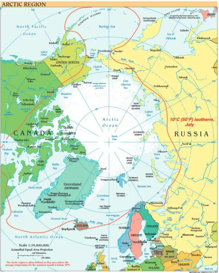
There are several definitions of the Arctic. In general it is the area farther north than the polar circle (66.56◦N). Whereas the climatological Arctic is the area on the northern hemisphere with a mean summer temperature less than10◦C and an area with a permanent frozen ground.
Because the warm gulf stream is heading northwards, subtropical atlantic water is transported to higher latitudes. The boundary of the climatological Arctic is much more shifted to the North in the European continent compared to Siberia or Northern America. In the following the climatological definition is used to determine the Arctic which is shown in figure 5.
The Arctic climate is dominated by the annual changes of incoming solar radiation between polar day and night during summer and winter times, respectively. The large temperature gradient between equator and pole is the main contributor to the atmospheric circulation. In the beginning this meridional flow is forced by the rotation of the earth and consequentially by the Coriolis force on a more zonal flow. During winter times the polar atmosphere is in stagnation. Based on the high albedo of the snow cover the surface layer constantly cools and the atmosphere is stable stratified because turbulent mixing of atmospheric layers is inhibited (Shaw, 1995). The temperature gradient is maximal between equator and polar regions and thus leads to a stronger meridional flow than in summer. When the polar night in spring ends the global temperature gradient decreases and more warmer air can reach the Arctic. With these changes of winds aerosols produced in the South can be advected into the Arctic more easily and form the Arctic Haze in the beginning of spring (Quinn et al., 2007). On the other hand the wet aerosol deposition is reduced during polar night because precipitating clouds are less frequent than in other seasons (Shaw, 1995).
Due to the already in the introduction mentioned Arctic Amplification the polar atmosphere is very sensitive to even small changes in the temperature. Additionally, the surface albedo in the Arctic is very high over snow and ice covered areas. Contrary to mid-latitudes and the tropics aerosols have a warming contribution to the large-scale energy budget because they re- duce the initially high albedo. For this reason it is very important to look at aerosol properties and long term trends in polar regions.
Figure 5: Climatological Arctic is located within the red line (source: https://legacy.lib.
utexas.edu/maps/islands_oceans_poles/arctic_region_pol_2007.pdf)
3. Data Processing and Methods
3.1. Instruments
In general, there are two ways of observing aerosols: in-situ and remote sensing instruments.
For in-situ measurements an aircraft or balloon is needed to fly directly into the atmospheric layer containing the aerosol. With this method micro-physical and chemical properties, like size, shape, composition or index of refraction, can be determined directly and very precisely for example by using filters or particle sizers. But the atmospheric cover is very small. Using remote sensing instruments, like satellites or ground based instruments, nearly the whole Earth is covered. But, compared to in-situ measurements, with a lower accuracy.
Additionally there are two different types of optical remote sensing instruments - active and passive ones. Active instruments emit electromagnetic radiation and receive the signal backscat- tered by aerosols or clouds in the atmosphere. Lidar is an example of this category. On the other hand passive instruments measure light transmitted through the whole atmosphere. Sun, stars or the moon are sources for these types of instruments. Photometers or radiometers are examples of this category.
To describe the atmospheric radiation balance it is necessary to measure aerosol properties which change the incoming solar radiation. One of the most important properties is aerosol optical depth (AOD). There are several possibilities for measuring it like Lidar, sun and star photometers. Because every instrument measures different aerosol properties at different times and to reduce typical errors of each instrument, the results should be combined for a better un- derstanding of the Arctic Haze. To fill the measuring gaps in the polar night a star photometer is used with a small overlap in March and October with the sun photometer.
3.1.1. Raman Lidar "KARL"
Figure 6: Lidar "Karl" while main- tanance work (Photo: San- dra Graßl)
The multi-wavelengths Raman Lidar KARL ("Kol- dewey Aerosol Raman Lidar") consists of a Nd:YAG laser with10W in each of the wavelengths λ= 355nm, 532nm and 1064nm. Additionally, in the first two wavelengths the polarisation in parallel and perpendic- ular to the emitted laser beam is recorded.
In the homosphere the fraction of nitrogen, N2, is con- stant at 78%. In this part of the atmosphere the Ra- man shifted lines of N2 are also detected at387nmand 607nm and water vapour at 407nm and 660nm. The mirror has a diameter of70cm. The overlap is complete after about 700m altitude, whereas below a qualitative estimation of the backscatter coefficient using a Vaisala CL51 ceilometer is performed. More technical details on the system are given in Hoffmann (2011). The evalu-
ation is typically done with30mvertical and10mintemporal resolution. No further smoothing of the Lidar profiles has been performed as this can easily lead to wrong results as the derivation of extinction coefficients from Lidar is an ill-posed problem.
3.1.2. Sun Photometer
Figure 7: Sun photometer during a calibra- tion expedition in Izaña, Tenerife (Photo: Sandra Graßl).
Aerosol optical depth (AOD) is measured by a sun photome- ter, type SP1a by Dr. Schulz & Partner GmbH (http://www.
drschulz.com/cnt/) in 17 wavelengths between λ = 369nm to 1023nm with a field of view of 1◦×1◦ and a time resolution of 1 minute. The wavelengths λ = 381.5,722.2,946.2,962.4,1045.3 and 1089.4nm are omitted in this thesis because measured AOD has always been too high. In winter 2012/13 a new sun photometer was installed and just 10 of 17 wavelengths re- mained in the same wavelength range. Only the wavelength λ = 944.8nm, which is devoted to water vapour, is omitted in this thesis for the newer photometer. To calibrate the filters for water vapour additional measurements of this highly vari- able atmospheric constituent are required. With the remain- ing 9 wavelengths optical parameters like the AOD are com- puted. The instrument is calibrated regularly in pristine condi- tions at Izaña, Tenerife, via Langley method. A cloud screen- ing based on short scale fluctuations of the AOD is used as in Alexandrov et al. (2004). The uncertainty for the AOD is generally said to be around 0.01 (Stock, 2010; Toledano et al., 2012). However, this is the maximum error of the instrument because the fluctuations are much smaller by comparing data minute by minute under low or constant aerosol conditions.
Therefore, we conclude that even 1 minute data has a suffi- cient quality and we are going to present some results accor- dingly.
The number of individual measurements differs between a few hundreds, especially in March and September, to up to 12,000 in early summer. No trend in each month can be seen com- paring the amount of cloud-free measurements over the years. Only an annual cycle due to polar day and night is included in the data. To compare different types or properties of Arctic aerosols the months April, May and August were chosen as typical months for periods with, without haze and late summer, respectively. The months March and September are not chosen because the number of available measurement points is limited due to the beginning and end of polar night.
An automatic tracking system was installed to the sun photometer in 2004. Since then the number of measurements has been increasing significantly because the photometer runs flaw- lessly. Before that upgrade measurements were taken only during campaign activity. Due to
the instrument data is only available in clear sky conditions. In this regard the data should represent the real aerosol conditions. Only aerosols that are advected and processed within clouds or hygroscopic growth cannot be measured by this instrument.
As in this study we are interested in typical aerosol properties we have omitted few singular extreme events from the data with AOD500 >0.3 that originates from known and exceptional strong events. Both, the agricultural flaming of May 2006 (Stohl et al., 2007) and the forest fire of July 2015 Markowicz et al. (2016) yieldedAOD500 values around 1 which would significantly bias monthly averages. If AOD500 >0.3was detected after cloud screening the whole day was omitted. In total seven days during the period from 2009 to 2017 were deleted from the data.
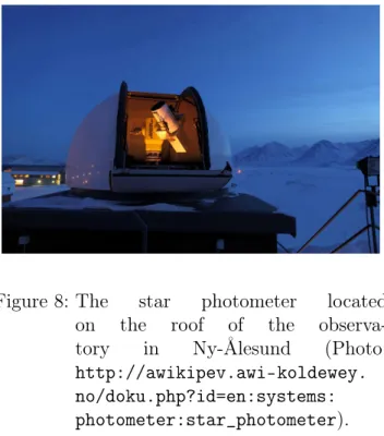
3.1.3. Star Photometer
Figure 8: The star photometer located on the roof of the observa- tory in Ny-Ålesund (Photo:
http://awikipev.awi-koldewey.
no/doku.php?id=en:systems:
photometer:star_photometer).
The measuring principle of a star photome- ter is the same as for the sun. It faces the star while rotating the different filters at λ = 420.0, 450.3, 469.4, 500.4, 532.1, 550.3, 605.4,639.8,675.7,750.9, 778.6,862.5, 933.2, 943.0, 952.7, 1025.9 and 1040.6nm.
With an additional background measure- ment the influence of stray light is re- duced.
There are two different possibilities to de- termine the AOD using a star photometer.
One star measurement requires a calibration at very clear nights, just like Langley calibra- tion for sun photometers. For the two star measurement a calibration is not needed in advance. But on the other hand the sec- ond method is much more effective by at- mospheric inhomogeneities and horizontally stratified layers.
The calculations of the AOD are performed very similarly to the sun photometer, only the apparent magnitude of different stars has to be taken into account.
To minimise measuring errors bright and, as a local advantage, circumpolar stars are chosen for photometry. The three stars γ Gem, β U M a and α Lyr are used for both types of mea- surement. The star α Aql has only been used for two star measurement yet. Their physical properties are shown in table 3.
apparent
star magnitude right ascension declination γ Gem (Alhena) 1.93 07h 34m 37.584s +31◦ 530 17.816000
β UMa (Merak) 2.37 11h 01m 50.476s +56◦ 220 56.733900 α Lyr (Vega) 0.04 18h 36m 56.336s +38◦ 470 01.280200 α Aql (Altair) 0.77 19h 50m 46.999s +08◦ 520 05.956300
Table 3: Position and apparent magnitude of all used stars for star photometry in Ny-Ålesund.
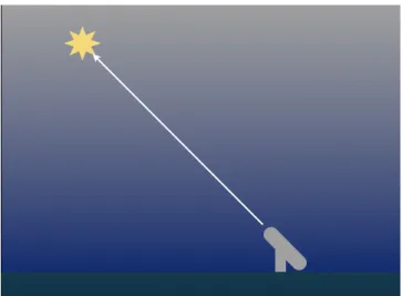
One Star Measurement
For one star measurements a Langley calibration, which is also commonly used for sun pho- tometers, has to be done in advance (see section 3.1.2).
Measurements for calibration taken by the star photometer in Ny-Ålesund are more scattered than measurements by the sun photometer. Thus, the error to the AOD is larger.
Figure 9: Measuring principle of a one star measurement
Due to the low apparent magnitudeM of stars compared to the sun a photon counter is used for measurements. The electronic count numberCN =SC−HC with SC is the total number of detected counts andHC the number of counts coming from the background, depends on the magnitude M:
M =−2.5·log10(CN) (3.1)
Using one star measurements and knowing the air massmand as well the measured apparent stellar magnitude M as the extraterrestrialM0, the total atmospheric optical extinction α can be computed for each wavelength:
αλ = Mλ−M0,λ mλ
=αAer +αRay+αO3 (3.2)
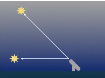
Two Star Measurement
A two star measurement consists of three standard measuring steps and requires as well a pair of stars with a high and a low star as a horizontal stratified, homogeneous atmosphere. Both stars should be as bright as possible and the following conditions towards each other:
1. Difference of the elevation angles as big as possible 2. Difference of the azimuthal angles as small as possible
Condition 1 arises from the calculation of the astronomical extinction coefficient. Only with the difference in the elevation of both stars the air mass can be calculated. Condition 2 should secure that the light of the two stars reaches the telescope under atmospheric conditions as equal as possible. For the calculation of the optical thickness of the aerosol the astronomical extraterrestrial magnitudes of both stars are needed. The steps of a two star measurement are:
1. Standard measuring of the low star (low1) 2. Standard measuring of the high star (high) 3. Standard measuring of the low star (low2)
Figure 10: Measuring principle of a two star measurement
The results are two values for the aerosol optical thicknesses per wavelength for each standard measuring pair of low1 to high and the standard measuring pair high to low2. Out of the high-graded two star measurings the spectral extraterrestrial magnitudes α1,2λ for the one star measuring are calculated which are used as calibration values for the one star measurement:
a1,2λ = (Mλ1−M0,λ1 )−(Mλ2−M0,λ2 ) m1λ−m2λ
=aAer+aRay+aO3 (3.3)
With the total atmospheric extinction the AOD can be determined:
τ1,2 =a1,2· ln(10) 2.5
=τAer+τRay+τO3 (3.4)
Cloud screening
Cloud screening is a crucial and difficult step in the preparation of data. An algorithm which is too strict removes all the data even if there are no clouds but a thick layer of aerosols. On the other hand a too soft algorithm does not remove all of the data with thin clouds and so conclusions of atmospheric properties get wrong.
The already existing algorithm for the sun photometer can not be applied to photometers dur- ing night times. Due to the large difference of stellar and solar irradiance the star photometer needs about6minfor one measurement whereas for the sun photometer only1minis sufficient.
In total only six star photometers are installed worldwide these days. Pérez-Ramírez et al.
(2012) has already suggested a cloud screening algorithm in three steps for the star photometer in Granada, Spain:
1 Eliminate all measurement points with values lower than their uncertainties and with air masses acquired withm <3.
2 Filtering of consecutive data points with ∆AOD(λ) > 0.03. Then moving averages for every AOD, τaer(λ), is computed for time periods of 1 hour and the whole measurement period. Data points are neglected when the difference between the data point itself and the average value is larger than 3 standard deviations.
3 Eliminate all data of this night if more than two-third are removed. Otherwise average remaining data over a time period of 30min.
During winter times the atmosphere is very stable without convection and the influence of the sun. Compared to aerosol arriving in Granada the background aerosol load in the polar air is much less and is less homogeneous which leads to a larger variability in the cases clouds arrive. Hence, the variability between two adjacent measurement points is small so that the steps 2 and 3 remove most of the data.
Therefore, a new idea has to be implemented using the measurements and the parameter α of equation 3.12 (chapter 3.2) directly.
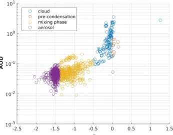
These thresholds are chosen by inspection of several measurement months of the star pho- tometer and by observations of Tomasi et al. (2007) who found characteristic values for different types of polar aerosols (table 5).
The clouds which are detected in the algorithm are still thin enough for the stellar light to pass through.
Type of measurement Properties
Cloud α >−0.5 and AOD500 >0.07 Pre-condensation α >0and AOD500 >0.07 Mixed phase α >−1.4 and α >−0.5 Aerosol α <−1.4 and AOD500 <0.1 Table 4: Parameters of the cloud screening algorithm.
Figure 11: Example of all measured data in November 2017. The different colours correspond to the thresholds listed in table 4
Before cloud formation takes place, the aerosol accumulates water vapour on its surface and rapidly changes its size, shape, refractive index and extinction efficiency. This effect only re- duces the visibility and increases the total optical depth. No cloud droplets are formed within this step but the photometer is not able to measure the AOD properly.
Manual cloud screening is very time consuming and also subjective, so an automatic script is needed. With this algorithm only data from Ny-Ålesund was analysed. To improve it, the Deutscher Wetterdienst (DWD) located in Lindenberg, Germany, is going to analyse and com- pare this algorithm with their own data. Even for them the cloud screening algorithm described in Pérez-Ramírez et al. (2012) is also too strict. A final evaluation will be done in future time.
In November 2017 the weather conditions were good enough to receive lots of data. The new cloud screening algorithm with the above mentioned thresholds are shown in figure 11.
To improve the thresholds of the four different categories this algorithm will have to be validated in future time.
Ozone correction
A huge problem during winter times is the missing of daily ozone measurements because sun light is needed for satellite based observations of a total ozone column. Only once a week an ozone balloon is launched in Ny-Ålesund.
Due to rapid changes of weather conditions the polar vortex rapidly changes its position and shape. Hence, the observing station Ny-Ålesund can be located within or onside the vortex and the vertical column of ozone can change from 178 DU (26.3.2011) to 785 DU (25.2.2009) in Ny-Ålesund.
The optical thickness of ozone is calculated with:
τo3 = Ko3(λ)
1000 ·O3(DU) (3.5)
Where Ko3(λ) being a wavelength dependent spectroscopic value based on the continuous Chappuis band between 400 and 650nm with the maximum at 603nm and O3(DU) being the total amount of ozone of the atmosphere in Dobson Units. The filter with the largest depen- dency of ozone of the star photometer has a wavelength of605.4nm, whereforeKo3(λ) = 0.1210.
For this particular filter of the star photometer the maximum error of a wrong ozone column concentration is∆τ = 0.0734 and, therefore, not neglectable.
Influence of PSCs on AOD
When the polar stratosphere becomes cold enough (<195K), water, nitric and sulphuric acid or even solid ice form spherical droplets and clouds in the stratosphere between 15-25 km height. They are called Polar Stratospheric Clouds (PSC). Over Ny-Ålesund they usually appear between December and March (Maturilli et al., 2005).
On the 23.12.2016 a PSC was observed via Lidar data with a thickness of about 0.5km over Ny-Ålesund while the star photometer was measuring simultaneously (figure 12). This day was chosen because the PSC was thickest at this day and is easily recognised in the Lidar profile.
The cloud screening algorithm detectes clouds between 10 and 10:30 am and the measured AOD is flagged afterwards as "mixing phase". Due to tropospheric conditions the star pho- tometer data was categorised into the above mentioned groups.
Knowing the thickness of the PSC (∆z = 500m), estimating the Lidar ratio (LR = 36) and in conjunction with the backscatter (baer = 2·10−7 m−1sr−1) the maximum optical depth for λ= 532nmof the cloud can be guessed using the equation for the definition of the Lidar Ratio:
LR= aaer
baer ⇒aaer =LR·baer Taking this result and using equation 2.3:
τP SC = Z z2
z1
aaer(z)dz '∆z·LR·baer = 3.6·10−3
While having an AOD variability between two adjacent measurements of up to 0.004, the influence of the PSC is negligibly small. Due to the small contribution of PSC to the total optical thickness this ansatz does not answer the question of a high mean AOD of this month.
(a) Lidar measurements of the PSC
(b) Star photometer measurement during the same time of the Lidar measurement
Figure 12: comparison of measured AOD during the presence of a PSC, observed by Lidar.
3.2. Data fitting and processing
The easiest way of fitting can be done with the later mentioned ansatz by Ångström. Never- theless, modified ways were implemented and tested to gain a bit more information and more accurate fitting results from given data.
All the used sun photometer data was evaluated with programs programmed by Maria Stock and Holger Deckelmann (Stock, 2010) in advance using World Meteorological Organization (WMO) standards (Hegner et al., 1998). So a correction of ozone was done using daily ozone column concentrations measured by the Total Ozone Mapping Spectrometer on a satellite operated by NASA. In the last step clouds were removed manually.
Ångström ansatz
The most obvious way to fit measured data by a photometer to a physical law is done considering Ångström theory in which extinction A and optical thickness τ is related to a reference value of a theoretical measurement at a wavelength ofλ0 = 1µmwith the ansatz by Ångström (1929, 1961, 1964):
τλ0 ·λ−A0 λ0 =τλ·λ−A
f(λ) =C·λ−A (3.6)
Where a = −ln(τ(λln(λ1)/τ(λ2))
1/λ2) and C =−λτ−Aλ =const. is the so-called turbidity parameter and it is connected to the refractive index, the total number of aerosol particles and its size dis- tribution. For A → −0 particles have at least the same size or are larger than the scattered light and so they are larger than 1µm (Stock, 2010) and the regime of geometrical optic can be
used. In this limes there is no wavelength dependency of scattering and both interference and refraction can be neglected. But geometrical shadows, transmission and macroscopic reflection become important. In the limes of A→ −4the particles appear like point masses and they are much smaller than the scattered solar radiation. This is also called the "Rayleigh regime". In a longterm study of Arctic aerosol properties at 500nmTomasi et al. (2007) found the Ångström exponent for Arctic background aerosol of A=−1.4 (table 5).
Aerosol Extinction Model AOD500 Ångström exponent A Mode Diameter[µm]
background Arctic aerosol 0.015 -1.40 0.01
Arctic dense aerosol 0.080 -1.00 0.01 and 0.60
Arctic Haze 0.150 -1.25 0.01 and 0.60
boreal smoke 0.300 -1.20 0.01 and 0.60
Table 5: Median values of Ångström Exponent A, AOD500 and mode diameter modeled by Tomasi et al. (2007).
This ansatz is commonly used in atmospheric science. But in the following different ways of AOD calculation are tested to increase the fitting accuracy and the gain of information about physical properties of aerosols.
Coarse and fine mode
Trying to gain additional information about aerosol properties an assumption concerning coarse and fine particle modes were done and described in O’Neill et al. (2001a), O’Neill et al. (2001b), O’Neill et al. (2003).
Optical properties of aerosols in the ultraviolet to the near-infrared spectrum are largely influ- enced by a fine and coarse mode (further described in section 2.1). The most important radius size is in sub-micron range.
The ansatz for coarse and fine mode is done using equation (O’Neill et al., 2001a):
τaer =τf +τc
=AfCf +AcCc (3.7)
where Af and Ac are the vertically integrated number density in abundance and Cf(λ) and Cc(λ) are the extinction cross sections of the fine and coarse mode, respectively. The indexes f and ccorrelate to fine and coarse mode and the Ångström exponentA is defined as:
A=−dlogτaer dlogλ with the second derivative:
A0 =−d2logτaer dlogλ2
The total optical curvature parametersτaer, A and A0 characterise most of the variability in the aerosol optical depth spectra and they are related to the coarse and fine mode components of the bimodal aerosol particle size distribution (O’Neill et al., 2001a). In O’Neill et al. (2003) all three parameters are referred to the measured spectrum to the reference values ofλ= 500nm in a second-order polynomial fit of ln(τaer)versus ln(λ).
This first method assumes a more flexible but necessarily more cumbersome optical descrip- tion in terms of independent discrete bins of a generalized aerosol size distribution.
The second method, and the more stable one, is a description of most optical phenomena by an appropriate choice of two or at most three size distribution modes. The second choice is more robust and repeatable than the multi-bin particle size distribution inversions of optical data and may serve the needs of many users of aerosol optical data (O’Neill et al., 2001a). The bimodal approach also permits simple and pure optical techniques to get coefficients for each separate particle size mode from the general spectral behaviour of the aerosol optical depth.
These coefficients can be used to extract microphysical parameters at an usually sufficient level, like effective or mean modal radius being derived from the Ångström coefficient associated with that mode.
Nevertheless, for the observations in the Arctic this algorithm was not used due to several reasons. First of all, O’Neill et al. (2001b) used a mono-cromatic ansatz to obtain a fitting ansatz for the polycromatic measurements. He argues that aerosol properties do not change from ultraviolet to near-infrared part of the electromagnetic spectrum (O’Neill et al., 2003).
Additionally, O’Neill et al. (2001a) also used algorithms for calculating Mie scattering to get an estimation for particle sizes (O’Neill et al., 2003).
In other polar regions, especially in North America, natural, like geophysical or biological, or anthropogenic processes create aerosol. This means a large distribution of particle radii.
Because of nearly no aerosol sources in Spitsbergen the arriving aerosols are very old and small.
Large particles are more affected by sedimentation or are washed out of the atmosphere by rain. So it is necessary in Ny-Ålesund to look at changes in AOD due to scattering of small and narrow distributed particles. Hence, the hypothesis is tested in the following whether A0 is independent of λ.
Long and short wavelength dependent Ångström ansatz
To prove whether a separation in wavelength is justified the original Ångström ansatz is taken but both parameters a1 and a2 are computed independently for two wavelength intervals (349,7nm ≤ λ1 ≤ 700nm and 700nm ≤ λ2 ≤ 1070,5nm). The intervals are chosen to ob- tain one for the visible range (VIS) of the electromagnetic spectrum and the other for the near-infrared (IR) part:
τ(λ) =
a1·λa2 , ∀λ <700nm
a3·λa4 , ∀λ >700nm (3.8) The four fitting parameters are calculated as in the traditional Ångström ansatz but inde-
pendently for every λ and for several days in 2013. For computating the fitting parameters the wavelength 675.9nm was included in both regimes. In case there is no difference be- tween Ångström ansatz and the modified one, in other words no wavelength dependency of the Ångström exponent is visible, a continuous fitting curve is expected.
However, the assumption of a power-law for the AOD is only a common approximation.
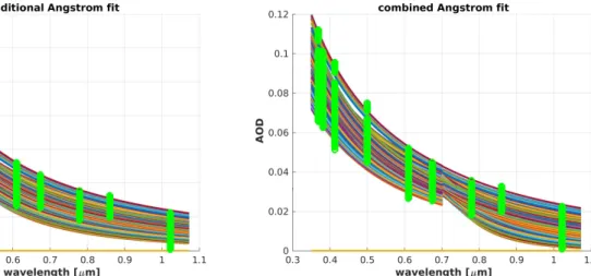
A typical result for arctic aerosol (green circles) can be depicted in figure 13. For simplicity the exponential fit (colored lines) is done using formula 1. It can easily be seen that this approximation under- and overestimates the measured AOD by the instrument (figure 13). To achieve a better result for the same data set the wavelength range was divided into two regimes, for the visible (<700nm) and infrared (>700nm) spectrum. Now two independent Ångström exponents are computed, one for every regime. The fitting curve with the chosen ansatz 3.8 approaches in a better way. In every case there was a step in the fitting functions of both regimes and the fitting accuracy has always been improved with this ansatz. Therefore, the fitting function 3.8 does not provide a good approximation of the aerosol properties and needs to be improved, why a wavelength independent ansatz has to be improved by an extension by a wavelength dependency.
The fitting accuracy is defined as the square differences χ2 between the observed and fitted AOD. In this thesis it is defined as:
χ2 = 1 m ·
n
X
k=1
AODmeas(λk)−AODf it(λk)
∆AOD(λk)
2
(3.9) Where m is associated with the degrees of freedom, n= 9 the number of used wavelengths, the suffixes ”meas” and ”f it” refer to the measured and fitted AOD, respectively. The error of the AOD is marked as∆AOD.
Differences in the fitting of the same data set with only two different wavelength intervals can be easily seen. Whereas the traditional ansatz (equation 3.6) can not reproduce a fit through the measured data in some cases, the new chosen ansatz of equation 3.9 can do so.
As it can be seen in the previous discussed generic days during spring and summer 2013 there is a change of fitting accuracy considering only long and short wavelengths, like in equation 3.8, compared to the general used Ångström ansatz in equation 3.6. This is an indicator that the suggested ansatz by Ångström (equation 3.6) has a wavelength dependent exponent.
Two component ansatz by Levenberg-Marquardt algorithm
Since an improvement was achieved by using equation 3.8 instead of equation 3.6, the Ångström law will be improved. This observation can be explained that the Arctic aerosol follows a bi- modal size distribution. Compared with other places worldwide the total aerosol load is much less but on the other hand there are sub-visible cirrus or ice crystals, which are very large.
(a) Data (green) with fitting curves (coloured) by Ångström law
(b) Data (green) with fitting curves (coloured) by two independent Ångström laws
Figure 13: Green circles represent individual measurements and the coloured lines the fitted exponential law. The data was fitted (a) in the full range of the photometer and (b) only in the visible (<700nm) and in the near infrared (>700nm) for the same data set.
To achieve a better fitting accuracy than by the traditional Ångström ansatz an approach was chosen using two components and the Levenberg-Marquardt algorithm for computation. It is a non-linear approach to find solutions for the non-linear fitting functionsf in the neighbourhood of an initially estimated parameter, in this particular case a1, a2, a3 and a4, in which f is a functional relation mapping a parameter vector to an estimated measurement vector.
Photometers only measure the integrated spectral AOD. In general it is possible that there are two independent layers of aerosols or aerosol and clouds lying over each other, which do not interact. For this case an equal looking summand is added to Ångström ansatz to gain independent information about both layers:
fLM(λ) = a1·λa2 +a3·λa4 (3.10) Considering the backscatter ratio measured by a Lidar it can easily determined whether aerosols or clouds are observed at this day.
For photometers cloud layers have to be sufficiently thin so that the direct solar radiation can penetrate the clouds directly. Otherwise the measured optical thickness is too large and the corresponding data point has to be removed out of the data set (Kautzleben, 2017).
To determine the convergence of the ansatz, the code has to come to the same result as the one with artificial noiseless data. Afterwards the noise increases linearly following the equation:
ftest(λ) =fartif icial(λ) +n·τnoise(λ) (3.11) Where fartif icial(λ) is the AOD computed by Levenberg-Marquardt algorithm being in the interval [0.0156 : 0.0859] for λ = 1019.0nm and λ = 368.1nm, respectively. r(λ) is a random
number individually set for each wavelength in the interval [−0.0956 : 0.2304] andn the factor tuning the signal-to-noise ratio. With this artificial AOD the algorithm has to converge to the four fitting parameters a1, a2, a3 and a4 of tauartif icial(λ) depending on the noise level n.
Table 6 shows whether the code still can achieve an acceptable result depending on the strength of the added noise:
n 1 10−1 10−2 10−3 10−4
convergence no no no yes yes
Table 6: convergence of the Levenberg-Marquardt algorithm with linear weighted noise added to AOD
Besides, Levenberg-Marquardt algorithm for equation 3.10 has a better fiting accuracy than Newton method, even noise in the order of 10−3 relative to the measured AOD disturbs the calculation and the code does not converge anymore. The two-component ansatz in theory is better but the convergence is only ensured when ∆ττ =O(10−3).
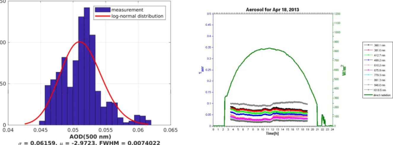
On a very clear day, like 18th April 2013, between 8 and 10 am all 120 measurements were taken to estimate the maximal error of the AOD at the reference wavelength of 500nm. Con- sidering a perfect sun photometer all the noise is produced by the atmosphere.
(a) Histogram ofAOD500nm for 18th April 2013 (b) Behaviour of the daily irradiance and the mea- sured photometer data
Figure 14: 18th April 2013 as an example of a very clear day with only small fluctuations in all 10 wavelengths (right) and the corresponding histogram (left)
Looking at numerous days between spring and autumn the algorithm failed due to missing convergence of the fitting parameters or unphysical results such as:
• Extremely large exponents (a2, a4 ≥100) with small optical thicknesses (a1, a3)
• One of the prefactorsa1 ora3 is negative when the corresponding exponents are very close to each other a2 ' a4. In the limes of small differences this algorithm becomes equal to the linear fit with only one summand.
To summarise the ansatz with two components is not an improvement to the traditional Ångström law in equation 3.6.
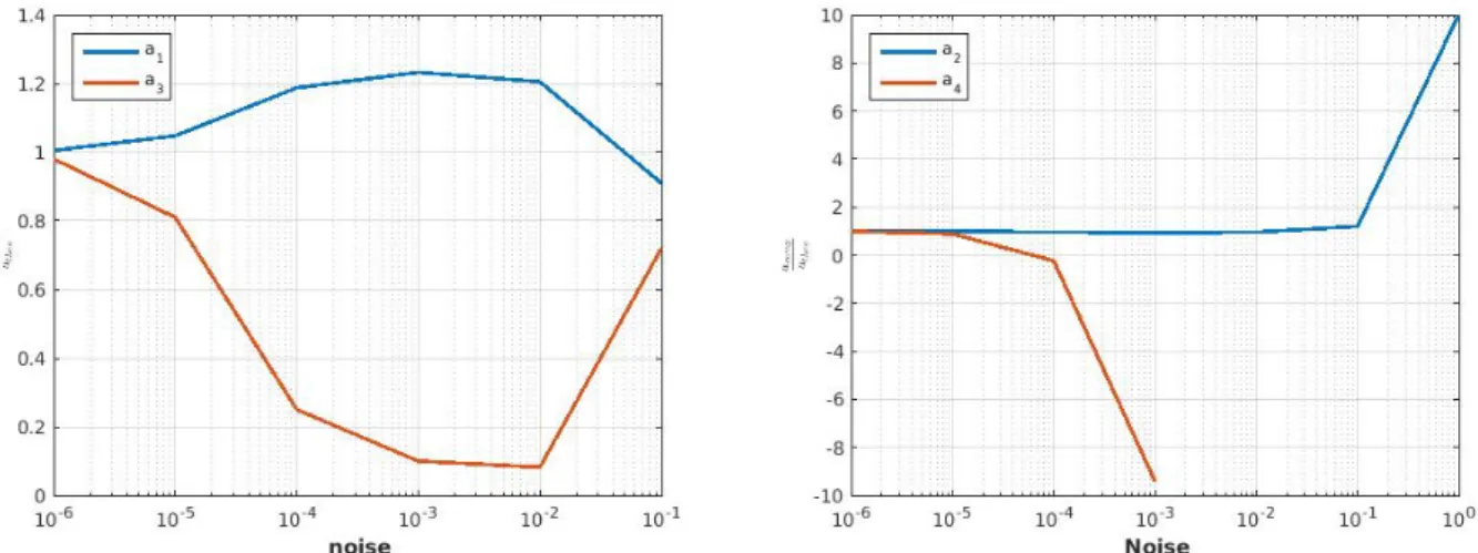
Figure 15 shows the fraction of the previously assumed parameters to the calculated ones as a fluctuation of the added noise to the AOD. The graphs of figure 15 in blue are the first summand and red the second one of equation 3.10.
The error for first summand with a1, allocated with aerosol, anda2, connected to clouds, in all cases is much smaller than for the second one, which also diverges first.
Figure 15: Quotient of computed to artificial parameters fora1, a3 (left) and a2, a4 (right) The clear day was used to give the scatter of the AOD expecting 0.007 which is approxi- mately 1% of the AOD but the code converges only at 10−3. This means the chosen ansatz (equation 3.10) is nice, physically motivated but requires one order of magnitude more precise measurement data until Levenberg-Marquardt algorithm will have a chance to retrieve the cor- rect solution from the observation data. Hence, this algorithm, as it is, is not suitable for the sun photometer standing in Ny-Ålesund.
With an improved photometer this algorithm can become useful for two constituents within the atmosphere and therefore two independent parameter sets for extinction and AOD. Im- provements could be more measured wavelengths for fitting because in this case the code has more fix points and the fit curve is more accurate. Another possibility is a better resolution due to less technical noise production within the instrument. To get more information about the technical noise itself a calibration in a laboratory can also be done previously.
Wavelength dependent Ångström exponent
As a result of the clear improvement of the ansatz by Ångström (equation 3.6) with two in- dependent components in equation 3.8, now a wavelength dependent Ångström exponent is
assumed and an ansatz with three wavelength independent fitting parameters C, α and β is chosen:
flin(λ) = C·λα+β·λ (3.12)
A Taylor expansion in the wavelengthλ was done to Ångström ansatz in 3.6, leaving in zero order a constant parameter α with the same meaning as the Ångström exponent. It can also reach values in the interval[−4 : 0]. In the first order the correction is done byβ·λwithβbeing the first derivative ofα. βbecomes more important the larger the wavelength dependency gets.
Hence, the correction term is mostly effective to the infrared. The constant C is the same as in Ångström ansatz and does not depend on the wavelength.
(a) Convergence ofα (b) Convergence ofβ
(c) Artificial AOD calculated by the Mie pro- gram of libRadtran
Figure 16: Convergence behaviour of the algorithm for both parametersα (a) andβ (b) for the given AOD500 shown in (c)
For each minute during one day within up to 400 iterations or a difference of at least 10−11 between two computational steps the best fit for all three parameters C, αandβ is numerically
computed again by Levenberg-Marquardt algorithm because only the elements of the Hesse matrix in this algorithm change. Instead of evaluating the second derivatives of the fit function fartif icial(λ) in equation 3.10 due to a1, a2, a3 and a4 now the second derivatives of flin(λ) in equation 3.12 to C, α and β are used.
To ensure the data has no noise, an artificial atmosphere was assumed calculated by the Mie program of libRadtran (see chapter 3.3). The given AOD is shown in figure 16c.
Figure 16 shows the convergence behaviour of the fitting equation 3.12 until the difference between two consecutive values does not change more than 10−11 anymore for all three pa- rameters C, α and β. For this particular chosen AOD the code already reaches the final value after the third step. All of the following computations are only necessary for vernier adjustment.
After checking for artificial atmospheric conditions all real photometer data between 2009 and 2017 were computed with this wavelength dependent ansatz of the Ångström formula (equa- tion 3.12). In 254,312 of all 255,389 cases (99.58%) a clear improvement was found like it can be seen in figure 17 for the 25th April 2015.
Figure 17: Example of a day with changes in atmospheric conditions and an improvement in fitting accuracyχ2due to wavelength dependent ansatz. Due to errors in the Langley calibration a daily pattern can be considered in the fitting accuracy of the data (Kreuter et al., 2013)
Therefore, the approach of the modified Ångström exponent and its spectral slope reveals is used for computing the AOD in this thesis because more information can be gained out of the measurement.