AEROSOL INVESTIGATION DURING THE ARCTIC HAZE SEASON OF 2018: OPTICAL AND HYGROSCOPIC PROPERTIES

(1)

AEROSOL INVESTIGATION DURING THE ARCTIC HAZE SEASON OF 2018: OPTICAL AND HYGROSCOPIC PROPERTIES

Kim Janka Müller^1,2*, Christoph Ritter¹, Konstantina Nakoudi^1,3

1Alfred Wegener Institute, Helmholtz Centre for Polar and Marine Research, Potsdam, Germany

2Carl von Ossietzky University, Oldenburg, Germany

3Institute of Physics and Astronomy, University of Potsdam, Potsdam, Germany

*Email: kim.janka.mueller@alum.uol.de ABSTRACT

In the beginning of March 2018, Lidar measurements were performed on Svalbard, Arctic Ocean, in order to analyse the optical and hygroscopic properties of Arctic aerosol. In this study, aerosol backscatter showed signiﬁcant higher values in lower altitudes. The analysis of the Colour Ratio (CR) revealed smaller particles in lower altitudes, with larger particles appearing only above Investigation of the hygroscopic character was done by applying the growth parameter introduced by Gassó et al.

(2000). It was found that the method of Zieger et.al. (2010) can be successfully extended to backscatter and CR data from Lidar measurements. Ice nucleation was examined in ice supersaturation conditions, with no ice cloud formation observed. This indicated that the role of Arctic aerosol as ice nuclei is still a poorly understood issue.

1. INTRODUCTION

During springtime, aerosol containing air masses are transported into the Arctic troposphere, forming the Arctic Haze. The main sources are suggested to be anthropogenic, originating from i.e. biomass burning, industry, heating, and forest ﬁres from Eastern Europe or Siberia. [1]

Arctic Haze lasts from February to April with its peak in March [2]. Polluted particles are mainly found below [3]. Arctic is a sensitive area experiencing significant changes in the radiation budget [4]. The phenomenon of Arctic Amplification describes the increase of near- surface temperature in Arctic regions compared to lower latitudes [5]. Increasing temperature leads to an earlier melting of sea ice and hence to a smaller albedo [6]. Since aerosol contribution to Arctic Amplification is not fully understood, it is important to analyse the optical, microphysical and hygroscopic properties of

Arctic aerosol especially during the Haze period [7], [8] and [9].

2. INSTRUMENTS KARL

The Lidar system used to collect the data for aerosol analysis is called KARL (Koldewey Aerosol Raman Lidar). This Lidar is operated at the AWIPEV station in Ny-Ålesund, Svalbard in the European Arctic ( ). KARL is a “3β+2α+2δ+2wv” Raman Lidar using a Nd:YAG laser, which emits radiation at the wavelength of . By frequency doubling and tripling the wavelengths of and become available, which are subsequently being detected in parallel and perpendicular polarising states [10]. Aerosol backscattering was determined by the numerical stable method of Klett [11] with resolution. The backscatter coefficients can be used to define the Colour Ratio (CR, Eq. 01) [1].

(Eq. 01) λ₁ denotes the shorter wavelength and λ₂ the longer wavelength, z the distance travelled by laser light. Taking into account the spectral dependency of aerosol interaction with light, the CR provides an estimation of the aerosol size [12]. Throughout the collection of this study’s data, KARL mainly measured during night time in order to provide a clear measurement set without the impact of day stray light.

Radiosondes

During the Lidar measurement period, radiosondes were launched four times a day in March 2018 at and

EPJ Web Conferences 237, 02001 (2020) ILRC 29

https://doi.org/10.1051/epjconf/202023702001

(2)

UT in the framework of the year of polar prediction. The radiosondes were Vaisala RS-41 type. Various meteorological parameters as air- pressure, temperature, relative humidity (RH) and wind speed were obtained. RH over water was taken from the radiosonde as well as the RH over ice was determined, using the water vapour partial pressure (P) in hPa and the saturation pressure of ice (SP_ice):

(Eq.02) This work considers Lidar and radiosonde data taken between and of March 2018.

3. METHODOLOGY

Some aerosol types exhibit a hygroscopic character, which means that they attract water.

After a certain threshold of humidity, aerosol particles potentially start growing with their scattering efficiency changing [13]. Zieger et al.

(2010) determined a growth factor ( ) as in Eq. 03 using the aerosol’s diameter in wet ( ) and dry ( ) surroundings [14].

(Eq.03) Dry surroundings were defined in a humidity range of and wet surroundings within [1]. In this study, the growth factor was extended by the growth function ( as in Eq. 04, with γ denoting a hygroscopic growth parameter. High values indicate strong hygroscopic growth, whereas smaller show weak hygroscopicity [15].

(Eq. 04) Since the particle’s size was not available by Lidar data, the application of the growth function was extended to backscatter and CR data. This modification was associated with the dependency of backscattering and CR on RH.

Eq. 03 was transformed into Eq. 05 and Eq. 06.

(Eq.05)

(Eq. 06)

4. RESULTS

4.1 Statistical Overview of Optical Properties Histograms (Fig. 01) provide a statistical overview of aerosol backscatter during the measurement campaign. Four different height ranges were set to distinguish the behaviour of aerosol backscatter between different altitudes.

The analysis of backscatter (Fig. 01) showed that lower altitudes feature higher backscattering, indicating that due to the haze higher number of aerosols were observed compared to other seasons e.g. summer.

Fig.01: Distribution of aerosol backscatter in different altitude intervals.

Additionally, the analysis of CR showed high values for lower altitudes, indicating that mainly smaller particles were present. Only in an altitude higher than smaller CR values were found, indicating bigger particles.

Statistical analysis of the aerosol linear depolarisation ratio revealed that most of the observed aerosol were characterised by low depolarisation values, indicating spherical particles (only % of the data showed values of indicating aspherical particles).

4.2 Hygroscopic Growth

The hygroscopic character of aerosols allows investigating the dependency of their properties on the ambient humidity. Taking the growth function and parameters as described in Eq. 04 and 05, the dependency of backscattering (Fig.

02) and CR (Fig. 03) on humidity were investigated. Additionally, the number of data points for each growth parameter were determined and are listed together with the distribution of particles (Tab. 01) for data points

2

(3)

with Concerning aerosol backscattering, a weak hygroscopic behaviour was dominating ( revealed a weak hygroscopic parameter γ1). Nevertheless, strong hygroscopicity was apparent for a number of cases ( for ; non-valid data ).

Considerable is the distribution of all measured data (backscattering and CR), showing that the majority ( ) was found in a range of RH lower than . In the range of lay contained , while in a very humid surrounding only was found.

Fig.02: Backscattering versus humidity with fitted growth functions for different growth parameters.

Concerning CR (Fig. 03), its dependency on relative humidity was less pronounced compared to that of backscattering. The same formalism as in Eq.04 was applied but with a different sign for γ. It should be noted that the majority ( ) showed strong hygroscopicity . This showed that Zieger’s method can be applied to CR data as well (non-valid data ).

Fig.03: Same as Fig. 02, except for Colour Ratio.

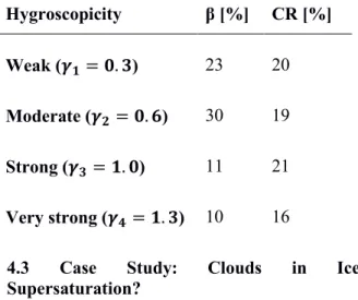
Tab. 01: Distribution of backscatter and CR for different growth parameters (for ).

Hygroscopicity β [%] CR [%]

Weak ( ) 23 20 Moderate ( ) 30 19 Strong ( ) 11 21 Very strong ( ) 10 16

4.3 Case Study: Clouds in Ice Supersaturation?

A case study examining the aerosol ice nucleation efficiency was analysed.

Fig.04: Backscattering in a time range of ±25min where the radiosonde (22:45UTC) was launched.

Depolarisation was investigated whenever high RH_ice was found, so as to determine whether an ice cloud was present or not. (Fig. 04) maximised at ( at 22:48 UTC, while in the time range of ca. ±10min significant lower values were recognised. Simultaneously, (Fig. 05) indicated supersaturation at 3.5km, whereas depolarisation (Fig. 06) was considerably low ( ) around 3km.

Despite supersaturation over ice, no ice cloud was observed. Water cloud formation could have happened within the time range of . Taking into account the dependency between humidity and temperature, temperature

3

(4)

fluctuations must have taken place to confirm this hypothesis.

Fig.05: Vertical profile of RHice. For comparison RHwater is shown.

Fig.06: Same as Fig.04, except for depolarisation.

5. CONCLUSIONS

In this study the aerosol optical and hygroscopic properties have been investigated during the Arctic Haze season 2018. The presented work revealed higher aerosol concentration in the first from ground, resulting from the presence of Arctic Haze. CR analysis indicated that most of the particles in lower altitudes were relatively small and only above bigger particles appeared. The application of the method of Zieger et al. (2010) [14] was extended to backscatter and CR data originating from Lidar measurements. The growth functions and their parameters were fitted into the present data set, with this adaption yielding satisfying results.

A case study concerning the aerosol ice nucleating efficiency indicated that not every aerosol type serves as ice nuclei. Thus, the indirect aerosol effect is still a poorly understood issue, since ambient conditions and aerosol type are potentially crucial factors.

APPENDIX

The aerosol depolarisation can be defined with Eq. 07 using the aerosol backscattering in parallel (ǁ) and perpendicular (⊥) polarisation as a function of the distance (z) and wavelength (λ).

(Eq. 07) Depolarisation is determined by the particle’s shape, thus conclusion about e.g. ice particles can be drawn [16].

REFERENCES

[1] M. Stock et al, Atmos. Env. 52, 48-55 (2011) [2] P. Tunved et al. Atmos. Chem. Phys, 13, 3643- 3660 (2013)

[3] W.R Leaitch et al. J. Clim. Appl. Met. 23, 916- 928 (1984)

[4] IPCC, Working Group 1, The Physical Science Basis (2007)

[5] S.R. Hudson, J. Geophys. Res. Atmos., 116, D16102 (2011)

[6] M.C. Serreze et al. Science, 315, 1533-1536 (2011)

[7] C. Ritter, et al. Atmos. Env. 141, 1-19 (2016) [8] J. Lisok et al. Atmos. Env. 140, 150-166 (2016) [9] K. Nakoudi et al. 29^th International Laser Radar Conference (ILRC 2019), Hefei, China (2019) [10] A. Hoffmann, Reports on Polar and Marine Research, 630, ISSN:1866-3192 (2011)

[11] J.D. Klett Appl. Opt. 31, No. 33, 211-220 (1981) [12] H.C. van de Hulst, Light Scattering by Small Particles (1981)

[13] climatescience, Aerosols and Climate, retrieved fromghttp://oxfordre.com/climatescience/view/10.10 93/acrefore/9780190228620.001.0001/acrefore- 9780190228620-e-13?rskey=FGAWKq&result=1 (2018)

[14] P. Zieger et al. Atmos. Chem. Phys., 10, 3875- 3890 (2010)

[15] S. Gassó et al. Tellus B, 53, 546-567 (2000) [16] J. Biele, Optics Express 7(12), 427-435 (2000) EPJ Web Conferences 237, 02001 (2020)

ILRC 29

4