Interannual and seasonal variations in the aerosol optical depth of the atmosphere in two regions of Spitsbergen (2002–2018)

(1)

https://doi.org/10.5194/amt-13-5303-2020

Interannual and seasonal variations in the aerosol optical depth of the atmosphere in two regions of Spitsbergen (2002–2018)

Dmitry M. Kabanov¹, Christoph Ritter², and Sergey M. Sakerin¹

1V.E. Zuev Institute of Atmospheric Optics, Siberian Branch of the Russian Academy of Sciences, Academician Zuev Square 1, Tomsk, Russia

2Alfred Wegener Institute for Polar and Marine Research, 14473 Potsdam, Germany Correspondence:Christoph Ritter (christoph.ritter@awi.de)

Received: 12 March 2020 – Discussion started: 25 May 2020

Revised: 8 August 2020 – Accepted: 18 August 2020 – Published: 8 October 2020

Abstract.In this work, hourly averaged sun photometer data from Barentsburg and Ny-Ålesund, both located on Spitsber- gen in the European Arctic, are compared. Our data set comprises the years from 2002 to 2018 with overlapping measurements from both sites during the period from 2011 to 2018. For more turbid periods (aerosol optical depth, AOD, τ0.5>0.1), we found that Barentsburg is typically more pol- luted than Ny-Ålesund, especially in the shortwave spectrum.

However, the diurnal variation in the AOD is highly correlated. Next, τ was divided into a fine and coarse mode. It was found that the fine-mode aerosol optical depth generally dominates and also shows a larger interannual than seasonal variation. The fine-mode optical depth is in fact largest in spring during the Arctic haze period. Overall the aerosol optical depth seems to decrease (at 500 nm the fine-mode optical depth decreased by 0.016 over 10 years), although this is hardly statistically significant.

1 Introduction

Studies of the character and causes of variations in all components of the climate system, including the aerosol composition of the atmosphere, have become more urgent with re- gard to climate change (IPCC, 2013). Atmospheric aerosol plays an important role in the processes of solar radiative transfer and exchange of different substances (in particular, pollutants) between the continents and ocean (e.g., Kon- dratyev et al., 2006). Compared with gases, aerosol is characterized by a complex physicochemical composition and a stronger variation in concentration and radiative impact.

Of the various aerosol characteristics, the observations of the aerosol optical depth (AOD) of the atmosphere are most widespread and are carried out at international and national networks of stations using sun photometers (see, e.g., WMO, 2005, and Holben et al., 1998). The AOD represents the extinction of radiation, integrated over the atmospheric column, and can be considered as an optical equivalent of the total aerosol content.

One of the main aerosol climatology problems is the determination of the specific features of interannual and seasonal variations in different regions. However, under changing climate system conditions, a 10-year (or even 20-year) time series may be insufficient to correctly identify the tendencies or periodicities in variations of aerosol characteristics.

The first observations of spectral AOD in the Arctic zone were carried out about 40 years ago (Shaw, 1982; Freund, 1983; Radionov and Marshunova, 1992); however, these observations only became regular in character in the early 2000s following the development of photometric observations at continental stations. A comprehensive overview of atmospheric AOD in the polar regions is given in Tomasi et al. (2012, 2015).

Studies by various authors have shown that the Arctic atmosphere is appreciably affected by outflows of different types of aerosols (e.g., smoke, industrial, sulfate and organic) from Eurasia and North America. The most powerful effect is due to smoke from forest fires that cover large areas of the boreal zone (e.g., Chubarova et al., 2012; Sitnov et al., 2013; Zhuravleva et al., 2017). The long-range transport of smoke plumes leads to considerable pollution of the Arctic atmosphere (Stohl et al., 2006; Stone et al., 2008; Eck et al.,

(2)

2009; Vinogradova et al., 2015). These episodes are short in duration (1–3 d) and rare because they depend on the product of the probabilities of two independent events: (a) a fire in any area of boreal zone and (b) the fact that the trajectory of air transport from a fire’s center arrives at a given region of the Arctic.

In addition to smoke, anthropogenic and other types of fine aerosol also flow out from midlatitudes. In contrast to forest fires, the sources of these aerosols operate almost all the time and are distributed over the entire territory of anthropogenic activity. A somewhat larger concentration of anthropogenic aerosol in densely populated regions of Europe has been observed during the past century; however, more re- cently, industrial emissions have stabilized or reduced in this area (Tørseth et al., 2012; Li et al., 2014; Zhdanova et al., 2019).

An AOD increase may also be associated with volcanic activity. In the period of time considered here, there were no large eruptions (such as the Pinatubo volcano in 1991) that had a global effect. The effects of less powerful volcanic eruptions on the Arctic atmosphere are short-term to mid-term (some weeks) in duration and are comparable to those due to smoke from forest fires. For instance, an AOD increase was observed on Spitsbergen after the eruptions of the Kasatochi (August 2008) and Sarychev (July 2009) vol- canoes (Hoffmann et al., 2010; Toledano et al., 2012).

The effects of pollutant outflows on the Arctic atmosphere intensify in the late winter–early spring. The temperature in- versions during this season lead to the formation and accumulation of aerosol in separate layers of the troposphere, which is known as the “Arctic haze phenomenon” (e.g., Shaw, 1995; Quinn et al., 2007; Tomasi et al., 2015).

Over the past decade, increasingly more work has been published analyzing the multiyear AOD variations in different regions, either based on spectral (Zhdanova et al., 2019;

Chubarova et al., 2016; Putaud et al., 2014; Li et al., 2014;

Xia, 2011; Michalsky et al., 2010; Sakerin et al., 2008a;

Weller et al., 1998) or integrated (actinometric) (Gorbarenko and Rublev, 2016; Plakhina et al., 2009; Ohvril et al., 2009) measurements of solar radiation. In most regions of Eurasia, the AOD shows a decreasing tendency after 1995. The nega- tive AOD trend is associated with a decreasing anthropogenic load and the absence of powerful volcanic eruptions analogous to Pinatubo (July 1991) and El Chichón (March–April 1982). Of particular interest is the dynamics of the aerosol constituent of the atmosphere in the Arctic zone, where the largest climate changes are seen (IPCC, 2013): increased temperature and a prolonged warm period, the reduction of sea ice area, changes in the circulations and so on.

Spitsbergen in the European Arctic is a special region, as it is strongly influenced by the warm West Spitsbergen Current.

Hence, for the given geographical latitude, the west coast of Spitsbergen faces warm and moist conditions. (Walczowski and Piechura, 2011). Moreover, Spitsbergen currently faces a pronounced winter warming of about 2^◦C per decade, which

can be partly explained by more efficient advection from the Atlantic Ocean (Isaksen et al., 2016; Dahlke and Maturilli, 2017). For this reason, aerosol properties over Spitsbergen may not be directly comparable to aerosol observations at other polar sites. On the other hand, we may see aerosol properties on Spitsbergen now that are more typical for the Arctic in the future under warmer, more marine conditions.

An analysis of aerosol properties for separate periods has already been performed for Spitsbergen (Herber et al., 2002;

Glantz et al., 2014; Chen et al., 2016; Pakszys and Zielinski, 2017). In this work, we discuss the AOD measurements from 2002 to 2018 in two regions on Spitsbergen: Ny-Ålesund and Barentsburg. Based on the multiyear observation time series, we considered the following issues: differences in the AOD between neighboring regions, the choice of the method for extracting the contributions of two (fine and coarse) AOD components, the seasonal average AOD variations during the polar day and the specific features of the interannual AOD variations during two periods of measurements (2002–2010 and 2011–2018).

2 Instruments, methods and observational data 2.1 Characterization of the instruments and regions of

measurements

Historically, observations of the spectral AODτ^a(λ)on the Svalbard archipelago have been carried out at three scientific stations that are located in close proximity to one another:

Ny-Ålesund (78^◦54⁰N, 11^◦53⁰E), Barentsburg (78^◦04⁰N, 14^◦13⁰E) and Hornsund (77^◦00⁰N, 15^◦34⁰E) – in the order of decreasing latitude. The distances from Barentsburg to Ny-Ålesund and Hornsund are 110 and 120 km, respectively.

Measurements of atmospheric AOD in the scientific settlement of Ny-Ålesund (population of about 100 residents during summer) have been performed since 1991. During the first stage of measurements (1991–1999), observations were performed during separate periods of the year (polar day and polar night) using different types of photometers (sun, lunar and star). The results of those studies have been considered in Herber et al. (2002). Here, we analyze the AOD variations during a later period when measurements became regular and homogeneous in character. The main characteristics of the sun photometers (SP1A and SP2H) used in measurements are presented in Table 1.

The sun photometer in Ny-Ålesund is located just south of the settlement at about 10 m a.s.l. on the Baseline Surface Radiation Network (BSRN) radiation field. The temporal res- olution of the data is 1 min. The instruments are regularly calibrated in Izaña/Tenerife. The air masses for aerosol and for ozone have been considered according to the formulas by Kasten and Young (1989) and the WMO (2008), respectively, and a cloud screening similar to Alexandrov et al. (2004) has been performed.

(3)

Table 1.Characteristics of the sun photometers and the data volume in Ny-Ålesund and Barentsburg.

Scientific stations Sun photometers Angle of Range of spectrum; number Number of hours (days) view (^◦) of spectral channels of measurements

Ny-Ålesund SP1A, 1 0.37–1.06 µm; 13 7520 (1130)

(AWI, Germany) SP2H 0.37–1.05 µm; 12

Barentsburg (AARI and IOA SPM, <2.5 0.34–2.14 µm; 11 1732 (350)

SB RAS, Russia) SP-9 <2 0.34–2.14 µm; 13

In 2011, the monitoring of aerosol characteristics (including AOD; Sakerin et al., 2018a) was organized at the Rus- sian Scientific Center, which is located in the southwestern part of Barentsburg settlement on the coast of the Grønfjor- den Gulf. Products of the coal mining industry and thermal power plant, which are located about 1 km from the monitoring site, may influence the aerosol characteristics in Barents- burg (population of about 500 residents).

The atmospheric AOD was initially measured using an SPM portable sun photometer (Sakerin et al., 2013) at an altitude of 65 m a.s.l. In 2015, it was changed to a SP-9 sun photometer with an automatic sun-tracking system (the instrument was installed at an altitude of 74 m a.s.l.). The base set of wavelength channels comprises the interference fil- ters with the passband maxima at the following wavelengths:

0.34, 0.37, 0.41, 0.50, 0.55, 0.67, 0.77, 0.87, 1.04, 1.25, 1.55 and 2.14 µm. Still another wavelength channel (0.94 µm) is used to determine the total water vapor content of the atmosphere.

The method for calculating the spectral AOD (Kabanov and Sakerin, 1997; Kabanov et al., 2009) includes consid- eration of the spectral transmission functions of light fil- ters as well as Rayleigh scattering and absorption by atmospheric gases: H₂O, O₃, CO₂and others. The absorption is calculated using databases of spectral line parameters HI- TRAN 2000 (https://hitran.org/media/refs/HITRAN-2000.

pdf, last access: 6 October 2020), models of continual absorption MT_CKD_3.3 (http://rtweb.aer.com/continuum_

code.html, last access: 6 October 2020) and vertical gas distribution AFGL (Anderson et al., 1986). Water vapor absorption is accounted for using real water vapor contents, measured in the 0.94 µm wavelength channel.

The data (hours and days of measurements) that were used for the AOD analysis in the two regions are presented in Ta- ble 1. Seasonal and interannual AOD variations were analyzed for the polar day (March–September) period. First, the hourly average AOD values were used to calculate the averages for each day of measurements, and the monthly averages were then calculated; based on the latter values, the averages for each year (more specifically, from March to September) were determined. For brevity, these values will be called daily, monthly, and annual AOD. The interannual variations in AOD were estimated in two variants: (a) according to the average values during the measurement period

(annual AOD) and (b) according to the averages in the periods of the spring maximum and fall minimum of AOD.

2.2 Data comparison and preparation of observation time series

A comparison of observations using two photometers may be of interest for the intercalibration of the instruments, i.e., estimating instrumental and methodical AOD determination errors (for the polar regions, e.g., Mazzola et al., 2011). If the measurements are separated in space (as in the given case), the difference in the data makes it possible to estimate local AOD inhomogeneities (Sakerin et al., 2010) caused by anthropogenic or natural factors such as local weather conditions, the type and state of the underlying surface, the orog- raphy, and the effect of industrial or other sources of aerosol.

It should be noted that we have already compared the AOD measurements at the neighboring stations on Spits- bergen, i.e., Hornsund and Ny-Ålesund (Toledano et al., 2012; Pakszys and Zielinski, 2017). The comparison of time- independent measurements showed that the average difference in the annual and seasonal AOD values at a wavelength of 0.55 µm does not exceed 0.01–0.02. Large differences in AOD between these stations occur during periods of Arctic haze and outflows of smoke from forest fires, which are man- ifest differently in these two regions. However, a comparison of monthly averages may introduce a bias due to different data availability at the involved sites.

In contrast to the abovementioned works, we compared quasi-synchronous (nearly time coincident) AOD measurements in the neighboring regions from 2011 to 2017 (see Ka- banov et al., 2018, for more details). The data from the SP1A (Ny-Ålesund) and SPM (Barentsburg) photometer observations were used to calculate the hourly average AOD values.

The data sets from the two regions were then compared provided that the times of the AOD measurements differed by no more than 1 h.

The comparison of the measurements from the two photometers showed a large dispersion of the data under strong atmospheric turbidity conditions, namely during the outflow of smoke plumes from forest fires and in the Arctic haze situations. Due to the large spatial inhomogeneity of these structures, the AOD (measured in two regions) may strongly differ, making the comparison incorrect. Therefore,

(4)

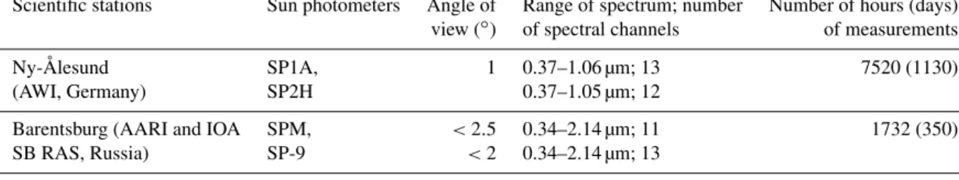
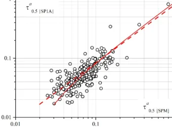
Figure 1.Scatter diagram of AOD measurements in two regions using SP1A (Ny-Ålesund) and SPM (Barentsburg) photometers. The solid line shows the unconstrained linear regression, and the dotted line shows the regression through the origin (0,0).

further analysis was performed for usual situations, whenτ^a (0.5 µm)<0.2. Figure 1 illustrates the regression relation between theτ^a(0.5 µm) measurements in neighboring regions on Spitsbergen.

A comparison of the statistical characteristics showed that the average AOD values are a little larger in Barentsburg than in Ny-Ålesund (Kabanov et al., 2018). The maximum difference in the AOD is observed in the shortwave part of the spectrum (0.38 µm), 1=τ^a (SPM) – τ^a (SP1A) =0.024, while the difference decreases to1=0.005 in near-IR range (0.87 µm). This feature is real despite the decreasing AOD at longer wavelengths, and it indicates that fine aerosol is more abundant in the atmosphere of Barentsburg. At the same time, we note that the AOD differences are minor (comparable with the uncertainty of determining AOD – about 0.01–

0.02; Kabanov et al., 2009; Sakerin et al., 2013), and the inter-diurnal AOD variations in the two regions are coordinated in character (correlation coefficients are between 0.83 and 0.89). Comparison of quasi-synchronous AOD measurements in Barentsburg and Hornsund gave close results (Ka- banov et al., 2018): 1=0.004–0.024, with correlation coefficients of between 0.71 and 0.81. Hence, observations in neighboring regions on Spitsbergen are quite compatible and identically reflect the specific features of the AOD variations.

The joint use of results from AOD monitoring in neighboring regions makes it possible to control the reliability of information as well as to identify the specific features of AOD variations not only for a specific site but for the region as a whole. The results of the observations in each of the regions have their own advantages. The advantage of the data from Barentsburg (SPM/SP-9 photometers) is a wider range (0.34–2.14 µm) of spectral measurements and the possibility to separate the contributions from two AOD components using an empirical method (see Sect. 2.3).

The valuable feature of the data from Ny-Ålesund is a longer AOD observation time series. However, different errors have accumulated in these data over the long measurement period. A simple exclusion of all suspect AOD measurements was undesirable because it was necessary to keep the observation time series as long as possible for the analysis of multiyear variations. Taking this circumstance into account, the multiyear observation time series was prepared to sort out or correct suspect AOD values (Kabanov et al., 2019a). The initial data set was processed to remove the data in which short-term bursts or rapid AOD variations were observed and to eliminate distortions to the smoothness of the wavelength dependences τ^a(λ). Owing to a certain redun- dancy of the number of spectral channels, we could identify false measurements and select most reliable data.

2.3 Fine and coarse AOD components

The attenuation of radiation by atmospheric aerosol varies as a function of wavelength, depending on the size and refractive index of aerosol particles. To characterize the AOD measured at different wavelengths, the Ångström formula is widely used:

τ^a(λ)=β·λ^−α, (1)

whereβandαare the approximation parameters of the spectral dependence of AOD;βis the turbidity coefficient, which is close in value to AOD at the wavelength of 1 µm; andαis the selectivity exponent (power law decay).

Numerous studies in different regions and under different atmospheric conditions have shown that Eq. (1) describes the wavelength dependenceτ^a(λ)in the main range (0.34–1 µm) of AOD measurements well (Ångström, 1964; Shifrin, 1995;

Eck et al., 1999; Cachorro et al., 2000; Schuster et al., 2006).

At the same time, the use of this formula has limitations and disadvantages that require an explanation.

First, the Ångström formula becomes unsuitable for de- scribing the wavelength behavior of AOD in the atmospheric

“transparency windows” in the wavelength range from 1 to 4 µm. This is because the power law dependence, Eq. (1), stems from the combined action of the fine and coarse aerosol fractions, which have different spectral properties. The extinction of radiation due to small particles (2π r/λ <1) is dominant in the visible region of spectrum; however, it rapidly decays with growing wavelength and becomes insignificant in the region beyond 1 µm. The extinction of radiation due to coarse aerosol barely changes with wavelength and becomes predominant in the near-IR range. Mie calculations and experimental data (Sakerin and Kabanov, 2007a;

Sakerin et al., 2008b) confirm that the power law AOD decay gradually transfers into almost neutral dependence. There- fore,τ^a(λ)in a wider wavelength range is better represented by the sum of two components:

τ^a(λ)=τ^c+τ^f(λ)=τ^c+m·λ⁻ⁿ, (2)

(5)

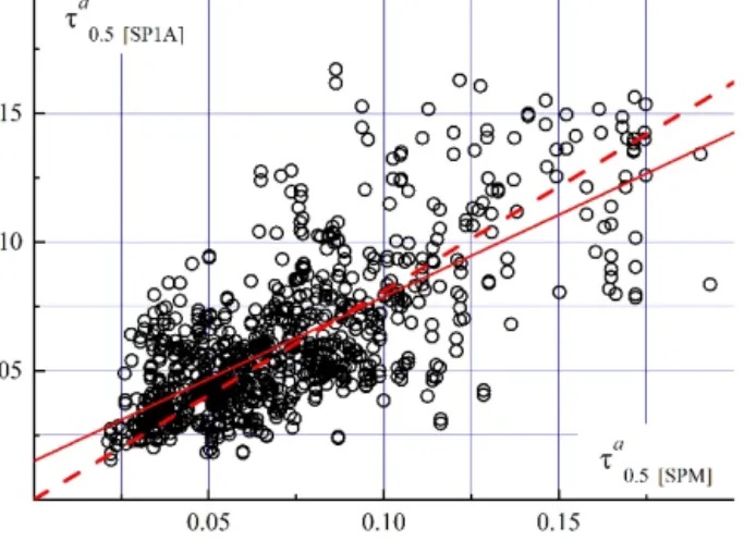
Figure 2.Correlation dependence between theαexponent and the ratio (τ_0.5^f /τ^c) according to measurements in Barentsburg. The solid line shows the unconstrained linear regression, and the dotted line shows the regression through the origin (0,0).

where τ^c is the constant (wavelength-independent) coarse AOD component,τ^f(λ)is the selective fine component, and mandnare the approximation parameters of the spectral dependence ofτ^f(λ)(and are similar to the parametersβandα of the Ångström formula).

Second, the Ångström parameters do not allow one to in- terpret the causes of AOD variations unambiguously. An increase or decrease in theαexponent is sometimes unjustifi- ably attributed to changes in fine aerosol alone. In fact, the αexponent conceals the actions of a few factors. The wavelength dependence of AOD is indeed determined by the optical properties of fine componentτ^f(λ). Both the size and refractive index of small particles influence the degree of AOD wavelength decay (and the values of thenandαparameters).

However, precisely what caused changes in the selectivity of AOD is almost impossible to determine without the use of additional information such as aerosol in situ measurements.

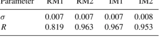
The next uncertainty factor is that theαexponent depends on the relationship of the optical depths of fine and coarse aerosol (τ_λ^f/τ^c). That is, α may increase both due to the growing content of fine aerosol and owing to the decreasing content of coarse aerosol. The presence of the interrelation between α and (τ_λ^f/τ^c) is illustrated in Fig. 2. The correlation coefficient between α and ln((τ_λ^f/τ^c)+1)is statistically significant and is equal to 0.68 (at a confidence level of P <0.0001).

We also note that theτ^ccomponent, which influences the αexponent, is tightly related and has values close to the second Ångström parameter (Sakerin and Kabanov, 2007a, b):

τ^c≈β. A consequence of this is that theαandβparameters are themselves correlated.

Thus, the use of the Ångström parameters in the analysis of AOD variations is ambiguous and may lead to erroneous conclusions. It is more preferable to consider the specific fea-

tures of the variations in the two AOD components:τ^f(λ)and τ^c. In addition to different sizes and spectral properties, fine and coarse aerosol fractions differ with respect to the ori- gins of particles and their transformation in the atmosphere.

Fine aerosol (e.g., sulfate and organic) is formed in the atmosphere as a result of various photochemical and microphysi- cal processes (Kondratyev et al., 2006). The lifetime of fine aerosol in the troposphere is a few days; therefore, it can be transported long distances (hundreds and thousands of kilo- meters). The main source of coarse aerosol (marine and dust) is the underlying surface. Because of its short lifetime and short transport distance, coarse aerosol is more local in character and pertains to a specific terrain. The only exceptions to this are powerful dust outflows from tropical latitudes.

2.4 Methods for determining fine and coarse AOD components

As indicated above, in the near-IR range, the effect of fine aerosol becomes insignificant, and AOD is determined only by the coarse component. Therefore,τ^c can be determined using an empirical method (EM), i.e., from minimal or average AOD values, measured in the range from 1.24 to 2.14 µm (Sakerin and Kabanov, 2007b; Sakerin et al., 2008b). Fol- lowing this, the second (fine) component can be found as a residual of the total AOD. Usually, it is estimated for the wavelength of 0.5 µm:τ_0.5^f =τ_0.5^a −τ^c.

However, most sun photometers (in particular the SP1A in Ny-Ålesund) operate in the wavelength range up to 1.05 µm, making an empirical method inapplicable. In this case, τ^c andτ_0.5^f can be estimated using calculation methods. For instance, in the AERONET system (http://aeronet.gsfc.nasa.

gov, last access: 6 October 2020), τ_0.5^f is calculated using the spectral deconvolution algorithm (O’Neill et al., 2003), based on the relationship of spectral AOD, measured in the shortwave part of the spectrum from 0.38 to 1.02 µm.

In Kabanov and Sakerin (2016), we suggested simpler methods for separating the contributions of τ_0.5^f and τ^c based on the regression interrelations with the parameters of Ångström formula. In the first regression method (RM1),τ^c is estimated using its interrelation with theβparameter (see Eq. 3 below). In the second method (RM2), the regression dependence ofτ_0.5^f on theα andβ parameters (see Eq. 4) is used. The comparison of different methods ofτ_0.5^f (orτ^c) estimation for marine and continental (Tomsk) atmospheric conditions showed close results: the average difference ofτ^c from data of the base empirical method (EM) does not exceed 0.007 for a standard deviation from 0.006 to 0.024.

For Arctic conditions (such as those at Spitsbergen), we performed an additional study (Kabanov et al., 2019a) regarding the selection of an optimal method of τ_0.5^f (or τ^c) estimation. Different methods were tested using SPM photometer measurements of AOD in Barentsburg. The error of the methods was estimated by comparing the calculated

(6)

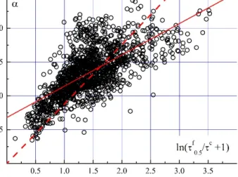
Table 2.Estimates of the applicability of different methods (RM1, RM2, IM1 and IM2) of theτ^c(orτ_0.5^f ) calculation.

Parameter RM1 RM2 IM1 IM2

σ 0.007 0.007 0.007 0.008

R 0.819 0.963 0.967 0.953

values of τ_0.5^f or τ^c with the data from the base empirical method.

Figure 3 illustrates the results of testing two regression methods (RM1 and RM2), based on the interrelations between τ^c and the β parameter and between τ_0.5^f and the α andβparameters. For the conditions on Spitsbergen, we obtained the following regression equations:

RM1:τ^c=0.665·β−0.0005 (3)

RM2:τ_0.5^f = −0.829+1.066·0.5^−α

·β (4)

Table 2 presents the standard deviations (σ) and the correlation coefficients (R values) between the calculated (RM1 and RM2) and empirical (EM)τ^cvalues. These results sug- gest that the regression methods make it possible to estimate τ^cwith an identical error of 0.007.

The disadvantage of the regression methods is that they require a preliminary data accumulation under the conditions of a specific region in order to determine the optimal regression coefficients in Eqs. (3) and (4) (Kabanov and Sakerin, 2016). Of course, the error of the regression methods may increase if the aerosol characteristics strongly differ from those typical for the region and do not correspond to the selected regression coefficients.

Therefore, in addition to the regression methods, we considered the applicability of another two methods ofτ_0.5^f estimation, based on the results of solving the inverse problem, namely the retrieval of the particle sizes from measurements of spectral AOD. Inversion method 1 (IM1) is based on the interrelation betweenτ_0.5^f and the volume or cross section of particles of fine aerosol. This method is implemented using the following steps:

– Step 1 – based on any known method of solving the inverse problem (for a specified refractive index, type of the particle distribution function and grid of radius ranges), the spectral AOD values are used to calculate the particle distribution function (dV /dr) or (dS/dr).

– Step 2 – in the distribution (dV /dr) obtained in Step 1, we select the part referring to the fine fraction and calculate the total particle volume (V^f) via integration.

– Step 3 – we consider the regression interrelation between particle volumes in the fine fraction (V^f) and the τ^fvalues, calculated using the empirical method (EM).

The interrelation obtained (Fig. 4a) is then used to select the parameters of a linear regression equation which

makes it possible to calculate theτ^fcomponent according to the particle volumesV^f.

Inversion method 2 (IM2) is implemented by first solving the inverse problem and then solving the direct problem of the aerosol optics; this is carried out as follows: as in IM1, the spectral AOD values are used to retrieve the distribution functions (dS/dr); based on the (dS/dr) values,τ_0.5^f is calculated for the size range of fine aerosol.

The inverse problem on retrieving the distribution functions (dS/dr) was solved using the iteration algorithm from Sviridenkov (2001), modified from the algorithm of Twitty (1975). The particle distribution was assumed to be lognormal, and the refractive index was assumed to have a real part of 1.5 and an imaginary part of 0. In the calculations we used the following radius grid: 0.09–0.13–0.17–0.21–

0.25–0.29–0.33–0.37–0.41–0.45–0.49–0.53–0.59–0.65–

0.81–0.99–1.21–1.59–1.81–2–2.5–3 µm.

The applicability of the inversion methods was estimated for a few variants: (a) for different wavelength intervals of AOD (0.34–2.14, 0.38–0.87, 0.38–1.02 and 0.34–1.02 µm), (b) for the distribution functions (dS/dr) and (dV /dr), and (c) for different radius boundaries of particles of the fine fraction (0.1–0.5 and 0.1–0.45 µm). Figure 4 presents examples of interrelations betweenτ_0.5^f (EM) and the calculated values of particle volumeV^fand betweenτ_0.5^f values determined using the respective base (EM) and inversion (IM1) methods.

The calculations in this case were performed for the AOD wavelength range from 0.38 to 1.02 µm and a particle radius range from 0.1 to 0.5 µm.

Analysis of the application of IM1 and IM2 (Kabanov et al., 2019a) showed that theτ_0.5^f determination error decreases by about a factor of 1.5 when the AOD is used in a wide (0.34–2.14 µm) wavelength range. However, for the narrower wavelength range of the SP1A photometer (0.38–1.02 µm) theτ_0.5^f calculation error is comparable with results from regression methods (see Table 2). That is, the relative errors of theτ^candτ_0.5^f calculations for the mean conditions of Bar- entsburg (τ_0.5^a =0.086; Sakerin et al., 2018a) are 30 % and 11 %, respectively.

The IM1 method was chosen for a subsequent use. Despite its more complicated calculation procedure, IM1 is more sen- sitive to aerosol variations, which is indicated by the highest correlation coefficient betweenτ_0.5^f (IM1) and data from the base (EM).

There may be a question as to why we consider the seasonal and interannual variations in the optical characteristics τ^candτ_0.5^f after the retrieval of the aerosol size distribution.

The analysis of the disperse composition of aerosol is a more complex and nonunique problem because it is necessary to consider the transformation of two aerosol fractions, which are described by a few parameters: the shapes and widths of the distributions for each fraction, the separation bound- ary and the effective particle radii. Moreover, an uncertainty

(7)

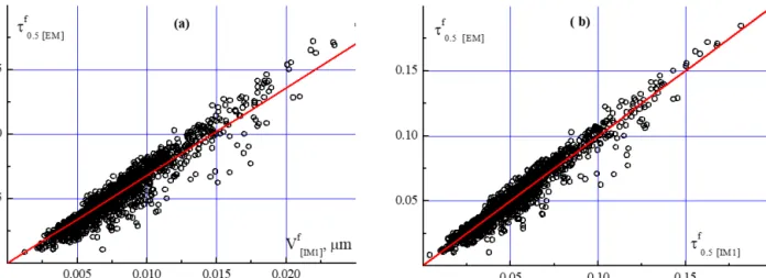
Figure 3. (a)The interrelation ofτ^cwith theβparameter, and(b)the interrelation ofτ_0.5^f calculated using the respective base (EM) and RM2 methods.

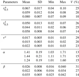
Figure 4. (a)The interrelation betweenτ_0.5^f and the particle volumeV^f, and(b)the interrelation betweenτ_0.5^f values calculated using the respective inversion (IM1) and empirical (EM) methods.

remains regarding the values of these parameters due the a priori specified aerosol refractive index.

In this work, we pursued a simpler task: to determine the character and magnitude of variations in aerosol optical characteristics. In this case, instead of many microstructure parameters, it is sufficient to analyze their more compact optical image in the form of two components –τ^fandτ^c.

3 Discussion of the results

Current climate change and environmental transformation influence the regularities of variations in aerosol characteristics to some degree. Due to the deficit of local aerosol sources in the Arctic zone, outflows of smoke and anthropogenic and volcanic aerosol from midlatitudes play an important role in AOD variations in this region. The frequency of these outflows in particular months and years determines the specific

features of the seasonal dynamics of AOD in Arctic regions and the magnitude of interannual oscillations.

3.1 Interannual variations

The highest atmospheric turbidities in the Spitsbergen region were observed on 10 July 2015 and on 2–3 May 2006 (Fig. 5). Daily AOD (0.5 µm) in these cases reached 0.82 and 0.6, respectively, which are values that are about an order of magnitude larger than multiyear averages. After passing to monthly AOD values, the effect of these short-term turbidities decreased to 0.192 in May 2006 and 0.152 in July 2015.

Trajectory analyses of air mass motion showed that the extreme AOD values in July 2015 were due to the long-range transport of smoke from forest fires in Alaska (Sakerin et al., 2018a; Pakszys and Zielinski, 2017; Markowicz et al., 2016).

We also considered the second anomalous situation (in May 2006) (e.g., Lund Myhre et al., 2007; Stohl et al., 2007) that

(8)

Figure 5.Spectral dependences of AOD: the top of the panel shows situations with high aerosol turbidities of the atmosphere, and the bottom of the panel shows the multiyear averages in the two regions.

was associated with the outflow of smoke aerosol from agricultural fires in the eastern Europe in detail.

Episodes with high atmospheric turbidities were also observed in June 2003, March and August 2008, April and Au- gust 2009, and April 2011. The AOD values during these periods of time have been analyzed by many authors (Toledano et al., 2012; Glantz et al., 2014; Tomasi et al., 2015; Chen et al., 2016; Pakszys and Zielinski, 2017). Independent of the causes of these short-term turbidities (Arctic haze and outflows of smoke or volcanic aerosol), they enhance not only the monthly but also the annual AOD values.

The abovementioned high-turbidity episodes (2006, 2008, 2009 and 2015) were partly reflected in annual AOD oscillations (Fig. 6). Moreover, a maximum appeared in the interannual variations in 2011–2012. This maximum was not due to extreme 1–3 d AOD bursts but to stronger turbidities compared with the adjacent years.

The annual AOD maxima occur with an average periodic- ity of about 3 years. When high-turbidity episodes are eliminated (see the dashed line in Fig. 6), certain maxima disap- pear; however, the general character of the AOD oscillations remains unchanged. Among these maxima, the highest AOD value in 2003 seems suspect. This annual AOD value can- not be considered representative due to the short observation periods (4 d in March and 5 d in May–June) in that year.

In addition to oscillations, a tendency toward a minor AOD decrease can be discerned in the multiyear variations (Fig. 6).

On average, the decline inτ_0.5^a is 0.016 over 10 years, but the significance of this trend is 0.062, which is close to but ex- ceeds the statistically significant level of 0.05. This is also indicated by a comparison of the AOD characteristics in the two observation periods: the average AOD (0.5 µm) in 2011–

2018 decreased by 0.013 relative to 2002–2010 (Fig. 5).

Overall,τ_0.5^f decreased by 0.016 over 10 years. However, this decreasing AOD tendency is hardly statistically significant

Table 3.Statistical characteristics of the annual AOD: average, minimal (Min) values, maximal (Max) values, standard deviations (SD) and variation coefficients (V). In each horizontal panel of the table, values for Ny-Ålesund (2002–2018) are shown in the first row, values for Ny-Ålesund (2011–2018) are shown in the second row and values for Barentsburg (2011–2018) are shown in the third row.

Parameters Mean SD Min Max V (%)

τ_0.5^a 0.067 0.017 0.04 0.10 25

0.059 0.012 0.04 0.08 20

0.080 0.007 0.07 0.09 10

τ_0.5^f 0.050 0.013 0.02 0.07 26

0.044 0.011 0.02 0.06 25

0.058 0.008 0.04 0.07 14

τ^c 0.017 0.005 0.01 0.03 29

0.015 0.003 0.01 0.02 20

0.022 0.005 0.01 0.03 23

α 1.41 0.19 1.03 1.71 13

1.44 0.21 1.11 1.71 15

1.24 0.19 1.01 1.60 15

β 0.026 0.008 0.016 0.040 31

0.022 0.006 0.016 0.034 27 0.035 0.005 0.025 0.042 14

(confidence level of 0.062). The statistical estimates of the τ_0.5^f andτ^c variations in the spring and fall periods in these two regions (Fig. 7) also revealed no trend component.

From the statistical characteristics (Table 3) and Fig. 7, it follows that AOD and its interannual variations are mainly determined by fine aerosol: the SD values and the range

<Min–Max> are a factor of 2–3 larger for τ_0.5^f than for τ^c. The relative variations inτ_0.5^f andτ^care about the same:

their variation coefficients (V values) are between 14 % and 29 %. Neither AOD component shows a clear predominance of variation coefficients. For instance, in the period from 2011 to 2018, the variation coefficients were larger forτ_0.5^f than for τ^c (25 % and 20 %, respectively) in Ny-Ålesund;

however, the inverse was found in Barentsburg, with values of 14 % and 23 %, respectively.

The interannual oscillations in the Ångström exponent can be considered minor: the variation coefficients for α are 13 %–15 %. The average α and the total variability range (from 1 to 1.7) are within the range of values characteris- tic for the continental midlatitude atmosphere and are larger than those in the marine atmosphere (Sakerin et al., 2018a, b). These Ångström exponent values are because the ratio (τ_0.5^f /τ^c=2.6–2.9) and the relative contribution of the fine component (τ_0.5^f /τ_0.5^a =0.73–0.75) are close to continental values. As an example, we present multiyear data in the boreal zone of Siberia during the spring (smoke-free) period (Kabanov et al., 2019b). The average AOD values in Siberia are about 2 times larger (τ_0.5^f =0.105,τ^c=0.036) than in

(9)

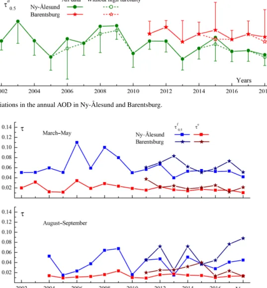
Figure 6.Multiyear variations in the annual AOD in Ny-Ålesund and Barentsburg.

Figure 7.Multiyear variations inτ_0.5^f andτ^cfor the periods of the spring maximum and fall minimum of AOD in two regions on Spitsbergen.

Ny-Ålesund, and the ratio (τ_0.5^f /τ^c) and theαexponent are almost the same: (τ_0.5^f /τ^c)=2.92 andα=1.43.

In Figs. 6 and 7, it is clearly seen that the AOD in Bar- entsburg is almost always higher than in Ny-Ålesund. The average excess of the annual AOD is1τ_0.5^a =0.02,1τ_0.5^f = 0.012,1τ^c=0.008 (see rows 2 and 3 in Table 3). This result indicates that slightly more anthropogenic (fine) and coarse aerosols are contained in the atmosphere of Barentsburg (see also Figs. 1 and 5).

Variations in the annual AOD in Ny-Ålesund and Barents- burg are coordinated in character. Oscillations in the fine component sometimes show inverse changes in the two regions, such as in spring 2013 (see Fig. 7). The different behavior ofτ_0.5^f may be because the observation time series are inhomogeneous in each region due to clouds or because the AOD values are measured at different times.

3.2 Specific features of seasonal variations

The most common regularity of the seasonal AOD behavior at midlatitudes is the spring (and sometimes also summer) maximum and fall minimum (e.g., Sakerin et al., 2015;

Chubarova et al., 2014; Holben et al., 2001). The primary causes of this AOD behavior are the annual cycle in the Sun’s declination, meaning a return of sunlight and possibly a longer aerosol lifetime over the frozen ocean. The springtime increases in insolation and temperature trigger a few processes: (a) snow cover evaporates and melts; (b) the atmosphere is enriched by different deposition products, which accumulated over the winter, (c) primary (marine and soil) aerosol starts to come from the underlying surface; and (d) photochemical production processes of in situ aerosol in the atmosphere and the emission of organic aerosol are acti- vated (e.g., Kondratyev et al., 2006).

(10)

Figure 8.Seasonal averageτ_0.5^a variations in Ny-Ålesund and Bar- entsburg.

The seasonal AOD dynamics in the Arctic zone is analogous to midlatitudes: there is a springtime maximum and a decay toward fall (e.g., Toledano et al., 2012; Tomasi et al., 2015; Sakerin et al., 2018a). This AOD behavior is due to similar annual rhythms of both local aerosol sources in the Arctic and long-range aerosol transport from midlatitudes.

Figure 8 shows the seasonal variations in monthly AOD for the two regions on Spitsbergen. The seasonal AOD behaviors in Ny-Ålesund were similar in character in 2002–

2010 and 2011–2018. The difference is that AOD values in March–June have decreased by ∼0.02 during the more recent 8 years. At the same time, monthly AOD in the second half of polar day (July–September) remained at the same low level (0.05–0.06). As a result, the seasonal AOD decrease in 2011–2018 became less pronounced: the relative amplitude had been 30 % – versus 55 % in the period from 2002 to 2010.

Seasonal AOD variations in Barentsburg are characterized by an additional summer maximum in July–August. Despite this difference, common factors in AOD variations in the two regions are nonetheless predominant. Analysis of the interrelation between AOD values measured in Ny-Ålesund and Barentsburg showed quite a high (0.90) correlation coefficient (Fig. 9). Hence, the synoptic, seasonal and interannual AOD oscillations are largely coordinated in character.

Observation time series from the two regions were compared to clarify the causes of the summertime AOD maximum in Barentsburg. The increased AOD values in July and August were found to be due to smoke outflows (in particular on 10 July 2015; Sakerin et al., 2018a). From the total number of measurements, the percentage of smoke-contaminated measurements was found to be larger in Barentsburg than in Ny-Ålesund. A few rare but powerful outflows of smoke aerosol led to an increase in the monthlyτ_0.5^f (Fig. 10) and τ_0.5^a (Fig. 8) values and distorted the natural seasonal variations. When these smoke outflow events were eliminated (see

Figure 9.The interrelation between daily AOD (0.5 µm) values measured in Ny-Ålesund and Barentsburg (2011–2018). The solid line shows the unconstrained linear regression, and the dotted line shows the regression through the origin (0,0).

Figure 10.Seasonal variations in the fine and coarse AOD components in Ny-Ålesund and Barentsburg.

the dashed lines in Figs. 8 and 10), the seasonal AOD behavior in Barentsburg became similar to that in Ny-Ålesund, although with larger (by 0.017 on average) AOD values. The average AOD characteristics for the spring maximum and fall minimum periods in the two regions are presented in Table 4 and Fig. 11.

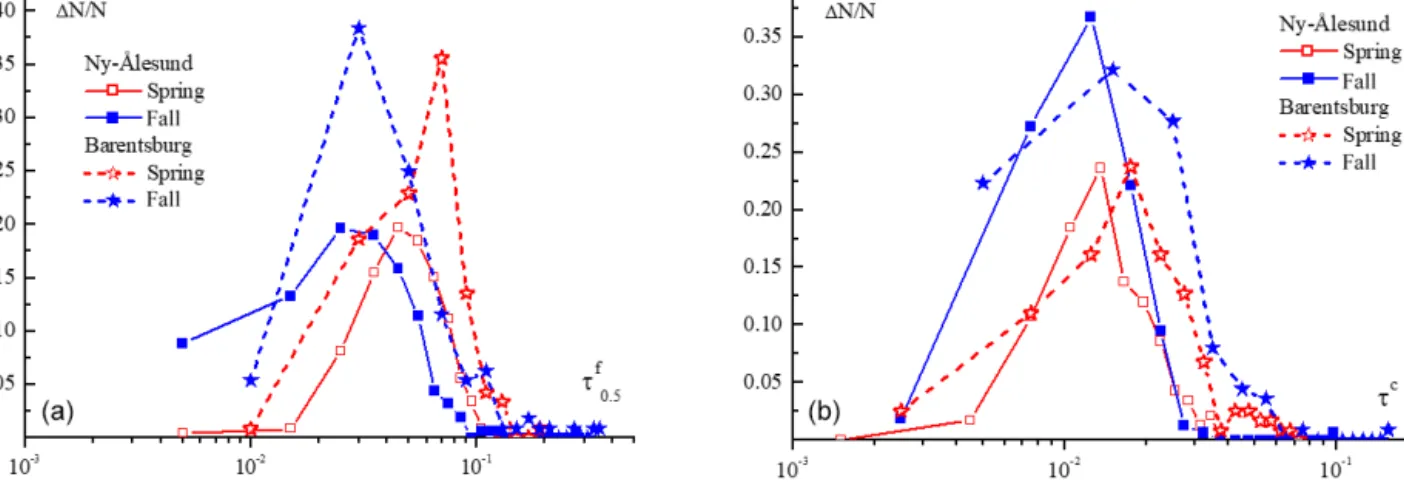
In Fig. 10 and Table 4, it can be seen that the fine component makes the major contribution to the formation of the seasonal AOD behavior: the average τ_0.5^f values decrease from spring toward fall in the two regions by almost the same amount (0.015–0.016). Moreover, modal (most prob- able)τ_0.5^f values vary in a similar way (Fig. 12a). Theτ_0.5^f mode from spring toward fall shifts from 0.07 to 0.03 in Bar- entsburg and from 0.05 to 0.03 in Ny-Ålesund. The average (Fig. 10) and modal (Fig. 12b) values of the coarse AOD component remain almost unchanged during the polar day:

(11)

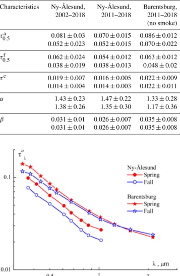
Table 4.Average AOD characteristics (±SD) in Ny-Ålesund and Barentsburg during the spring (April–May) maximum (first row in each horizontal panel) and fall (August–September) minimum (second row in each horizontal panel).

Characteristics Ny-Ålesund, Ny-Ålesund, Barentsburg, 2002–2018 2011–2018 2011–2018 (no smoke)

τ_0.5^a 0.081±0.03 0.070±0.015 0.086±0.012 0.052±0.023 0.052±0.015 0.070±0.022 τ^f

0.5 0.062±0.024 0.054±0.012 0.063±0.012 0.038±0.019 0.038±0.013 0.048±0.02

τ^c 0.019±0.007 0.016±0.005 0.022±0.009 0.014±0.004 0.014±0.003 0.022±0.011

α 1.43±0.23 1.47±0.22 1.33±0.28 1.38±0.26 1.35±0.30 1.17±0.36

β 0.031±0.01 0.026±0.007 0.035±0.008 0.031±0.01 0.026±0.007 0.035±0.008

Figure 11.Average spectral dependences of AOD in two regions on Spitsbergen (2011–2018) during the spring (April–May) maximum and fall (August–September) minimum.

monthlyτ^cvalues are about 0.015 in Ny-Ålesund and 0.022 in Barentsburg.

The seasonal decrease inτ_0.5^f from spring toward fall leads to changes in the ratio (τ_0.5^f /τ^c) and spectral AOD dependence (Fig. 11): the slope of the spectral AOD dependence and the Ångström exponent become a little smaller. The relative contribution of fine aerosol to AOD (τ_0.5^f /τ_0.5^a )in Ny- Ålesund is 0.77 in spring and 0.73 in fall. In Barentsburg this ratio is a little smaller – 0.73 and 0.69, respectively.

4 Conclusions

The following section presents a brief summary of the results of our study.

1. In order to identify the specific features of seasonal and multiyear variations in atmospheric AOD, it is important to analyze the fine and coarse AOD components separately, as they have different spectral properties, ori- gins and lifetimes. As applied to AOD measurements in Ny-Ålesund, we considered a few methods for estimating the contributions of fine and coarse components, and one of the methods (IM1) was selected for a subsequent use. A comparison with data from the base (EM) showed that the standard deviation of theτ^candτ_0.5^f calculations is 0.007, and the relative errors are 30 % and 11 %, respectively.

2. Outflows of different types of fine aerosol from the Eurasian and North American midlatitudes appreciably affect the monthly (and even annual) AOD in the Arc- tic atmosphere. Outflows of smoke from massive forest and agricultural fires have the strongest effect. The frequency of these episodic outflows in specific years as well as the frequency of of Arctic haze events influence the specific features of the seasonal variations and determine the amplitude of the interannual AOD variations in the Arctic atmosphere.

3. The oscillations in annual AOD in Ny-Ålesund and Barentsburg are coordinated in character and are determined by fine aerosol (interannual variations inτ^c are a factor of 2–3 smaller). In the multiyear (2002–

2018) variations we revealed a tendency toward decreasing AOD, but the trend is hardly statistically significant. The annual AOD in Barentsburg is, on average, 0.02 larger than in Ny-Ålesund, indicating larger fine (1τ_0.5^f =0.012) and coarse (1τ^c=0.008) aerosol contents in the larger settlement.

4. The seasonal AOD variations in Ny-Ålesund are characterized by a decrease from spring toward fall. In the last period (2011–2018), the seasonal AOD decrease became less pronounced. Monthly AOD values decreased from 0.07 to 0.09 (by∼0.02) in March–June, and they remained unchanged (0.05–0.06) in the second half of polar day. In the seasonal AOD variations in Barents- burg there was an additional summer maximum, which was caused by a relatively larger influence of smoke outflows. When the smoke outflow events were eliminated, the seasonal behavior became analogous to that in Ny- Ålesund, although with higher AOD values (0.017).

5. The fine component has the main effect on the formation of the seasonal behavior of AOD. Its relative contribution to AOD (τ_0.5^f /τ_0.5^a ) is 0.77 in spring and 0.73 in fall in Ny-Ålesund (0.73 and 0.69 in Barentsburg, respectively). The coarse AOD component during the polar day is almost unchanged: 0.015 in Ny-Ålesund and 0.022 in Barentsburg on average. The average annual and monthly values of the Ångström exponentα(from

(12)

Figure 12.Frequency histograms of(a)τ_0.5^f and(b)τ^cin spring and fall in two regions on Spitsbergen (2011–2018).

1.2 to 1.5) do not differ from those in the midlatitude continental atmosphere. That largeαexponents are because the ratios of the two AOD components (τ_0.5^f /τ^c) differ little between the Arctic and continental atmosphere.

Data availability. Data can be obtained from Dmitry M. Kabanov upon request.

Author contributions. DMK carried out the analysis and provided the figures. CR is PI of the photometer in Ny-Ålesund. SMS is the co-PI of the photometric measurements in Barentsburg. SMS and CR wrote the paper.

Competing interests. The authors declare that they have no conflict of interest.

Acknowledgements. The authors acknowledge their colleagues for organizing and carrying out the photometric observations in Ny-Ålesund and Barentsburg, namely Siegrid Debatin, Jürgen Graeser, Dmitry Grigorievich Chernov, Alexey Viktorovich Gu- bin, Konstantin Evgenievich Lubo-Lesnichenko, Aleksandr Niko- laevich Prakhov, Vladimir Fedorovich Radionov, Olga Ruslanovna Sidorova and Ury Sergeevich Turchinovich.

The study was supported by the Ministry of Science and Higher Education of the Russian Federation (project no. AAAA-A17- 117021310142-5).

Financial support. The article processing charges for this open- access publication were covered by a Research Centre of the Helmholtz Association.

Review statement. This paper was edited by Andrew Sayer and re- viewed by three anonymous referees.

References

Alexandrov, M. D., Marshak, A., Cairns, B., Lacis, A. A., and Carlson, B. E.: Automated cloud screening algorithm for MFRSR data, Geophys. Res. Lett., 31, L04118, https://doi.org/10.1029/2003GL019105, 2004.

Anderson, G., Clough, S., Kneizys, F., Chetwynd, J., and Shet- tle, E.: AFGL Atmospheric Constituent Profiles (0–120 km), Air Force Geophysics Laboratory, AFGL-TR-86-0110, Environmen- tal Research Papers, no. 954., 1986.

Ångström, A.: Parameters of atmospheric turbidity, Tellus XVI, 1, 64–75, 1964.

Cachorro, V. E., Duran, P., Vergaz, R., and de Frutos, A. M.:

Measurements of the atmospheric turbidity of the north-centre continental area in Spain: spectral aerosol optical depth and Angstrom turbidity parameters, J. Aerosol Sci., 31, 687–702, https://doi.org/10.1016/S0021-8502(99)00552-2, 2000.

Chen, Y. -C., Hamre, B., Frette, Q., Muyimbwa, D., Blindheim, S., Stebel, K., Sobolewski, P., Toledano, C., and Stamnes, J.:

Aerosol optical properties in Northern Norway and Svalbard, Appl. Opt., 55, 660–672. https://doi.org/10.1364/AO.55.000660, 2016.

Chubarova, N., Nezval’, Ye., Sviridenkov, I., Smirnov, A., and Slutsker, I.: Smoke aerosol and its radiative effects during extreme fire event over Central Russia in summer 2010, At- mos. Meas. Tech., 5, 557–568, https://doi.org/10.5194/amt-5- 557-2012, 2012.

Chubarova, N. E., Nezval’, E. I., Belikov, I. B., Gorbarenko, E. V., Eremina, I. D., Zhdanova, E. Yu., Korneva, I. A., Konstantinov, P. I., Lokoshchenko, M. A., Skorokhod, A. I., and Shilovtseva, O. A.: Climatic and Environmental Char- acteristics of Moscow Megalopolis According to the Data of the Moscow State University Meteorological Observa- tory over 60 Years, Russ. Meteorol. Hydro+., 39, 602–613, https://doi.org/10.3103/S1068373914090052, 2014.

(13)

Chubarova, N. Y., Poliukhov, A. A., and Gorlova, I. D.: Long-term variability of aerosol optical thickness in Eastern Europe over 2001–2014 according to the measurements at the Moscow MSU MO AERONET site with additional cloud and NO2 correction, Atmos. Meas. Tech., 9, 313–334, https://doi.org/10.5194/amt-9- 313-2016, 2016.

Eck, T. F., Holben, B. N., Reid, J. S., Dubovik, O., Smirnov, A., O’Neill, N. T., Slutsker, I., and Kinne, S.: Wavelength dependence of the optical biomass burning, urban, and desert dust aerosol, J. Geophys. Res., 104, 31333–31350, 1999.

Eck, T. F., Holben, B. N., Reid, J. S., Sinyuk, A., Hyer, E. J., O’Neill, N. T., Shaw, G. E., Vande Castle, J. R., Chapin, F. S., Dubovik, O., Smirnov, A., Vermote, E., Schafer, J. S., Giles, D., Slutsker, I., Sorokine, M., and Newcomb, W. W.:

Optical properties of boreal region biomass burning aerosols in central Alaska and seasonal variation of aerosol optical depth at an Arctic coastal site, J. Geophys. Res., 114, D11201, https://doi.org/10.1029/2008JD010870, 2009.

Freund, J.: Aerosol optical depth in the Canadian Arctic, Atmos.

Ocean, 21, 158–167, 1983.

Glantz, P., Bourassa, A., Herber, A., Iversen, T., Karlsson, J., Kirkevåg, A., Maturilli, M., Seland, Ø., Stebel, K., Struthers, H., Matthias, M., and Thomason, L.: Remote sensing of aerosols in the Arctic for an evaluation of global climate model simulations, J. Geophys. Res.-Atmos., 119, 8169–8188, https://doi.org/10.1002/2013JD021279, 2014.

Gorbarenko, E. V. and Rublev, A. N.: Long-term changes in the aerosol optical thickness in Moscow and correction under strong atmospheric turbidity, Izv. Atmos. Ocean Phy+., 52, 188–195, 2016.

Herber, A., Thomason, L. W., Gernandt, H., Leiterer, U., Nagel, D., Schulz, K., Kaptu, J., Albrecht, T., and Notholt, J.: Con- tinuous day and night aerosol optical depth observations in the Arctic between 1991 and 1999, J. Geophys. Res., 107, 4097, https://doi.org/10.1029/2001JD000536, 2002.

Hoffmann, A., Ritter, C., Stock, M., Maturilli, M., Eckhardt, S., Herber, A., and Neuber, R.: Lidar measurements of the Kasatochi aerosol plume in August and September 2008 in Ny-Ålesund, Spitsbergen, J. Geophys. Res., 115, D00L12, https://doi.org/10.1029/2009JD013039, 2010.

Holben, B. N., Eck, T. F., Slutsker, I., Tanre, D., Buis, J. P., Set- zer, A., Vermote, E., Reagan, J. A., Kaufman, Y. J., Nakadjima, T., Lavenu, F., Jankowiak, I., and Smirnov, A.: AERONET - A federated instrument network and data archive for aerosol characterization, Rem. Sens. Environ., 66, 1–16, 1988.

Holben, B. N., Tanre, D., Smirnov, A., Eck, T. F., Slutsker, I., Abuhassan, N., Newcomb, W. W., Schafer, J. S., Chatenet, B., Lavenu, F., Kaufman, Y. J., Vande Castle, J., Setzer, A., Markham, B., Clark, D., Frouin, R., Halthore, R., Karneli, A., O’Neill, N. T., Pietras, C., Pinker, R. T., Voss, K., and Zibordi, G.: An emerging ground-based aerosol climatology: Aerosol optical depth from AERONET, J. Geophys. Res., 106, 12067–

12097, https://doi.org/10.1016/S0034-4257(98)00031-5, 2001.

IPCC: Climate Change 2013: The Physical Science Basis, Inter- governmental Panel on Climate Change, 2013, 1552 pp. (elec- tronic resource), available at: http://www.climatechange2013.

org/images/report/WG1AR5_ALL_FINAL.pdf (last access: 5 October 2020), 2013.

Isaksen, K., Nordli, O., Forland, E. J., Lupikasza, E., East- wood, S., and Niedzwiedz, T.: Recent warming on Spits- bergen – Influence of atmospheric circulation and sea ice cover, J. Geophys. Res.-Atmos., 121, 11913–11931, https://doi.org/10.1002/2016JD025606, 2016.

Kabanov, D. M. and Sakerin, S. M.: About method of atmospheric aerosol optical thickness determination in near-spectral range, Atmos. Ocean Opt., 10, 540–545, 1997.

Kabanov, D. M., Veretennikov, V. V., Voronina, Yu. V., Sak- erin, S. M., and Turchinovich, Yu. S.: Information system for network sunphotometers, Atmos. Ocean Opt., 22, 121–127, https://doi.org/10.1134/S1024856009010187, 2009.

Kabanov, D. M. and Sakerin, S. M.: Comparison of assessment techniques of fine and coarse component aerosol optical depth of the atmosphere from measurement in the visible spectrum, in: Proc. SPIE., 22nd International Symposium Atmospheric and Ocean Optics: Atmospheric Physics, Tomsk, Russia, 100353D, https://doi.org/10.1117/12.2248657. 2016.

Kabanov, D. M., Sakerin, S. M., Kruglinsky, I. A., Ritter, C., Sobolewski, P. S., and Zielinski, T.: Comparison of atmospheric aerosol optical depths measured with different sun photometers in three regions of Spitsbergen Archipelago, in: Proc. SPIE., 24th International Symposium on Atmospheric and Ocean Op- tics: Atmospheric Physics, Tomsk, Russia, 13 December 2018, https://doi.org/10.1117/12.2503949, 2018.

Kabanov, D. M., Sakerin, S. M., and Ritter, C.: Preparing time series of observations of atmospheric aerosol optical depth (AOD) at two stations on Spitsbergen Archipelago and selecting methods of extracting the contributions of fine and coarse AOD components, in: Proc. SPIE., 25th International Symposium on Atmo- spheric and Ocean Optics: Atmospheric Physics, Novosibirsk, Russia, 18 December 2019, https://doi.org/10.1117/12.2539926, 2019a.

Kabanov, D. M., Sakerin, S. M., and Turchinovich, Yu, S.:

Interannual and seasonal variations in the atmospheric aerosol optical depth in the region of Tomsk (1995–

2018), Atmospheric and Ocean Optics, 32, 663–670, https://doi.org/10.1134/S1024856019060071, 2019b.

Kasten, F. and Young, A. T.: Revised optical air mass ta- bles and approximation formula, Appl. Opt., 28, 4375–4738, https://doi.org/10.1364/AO.28.004735, 1989.

Kondratyev, K. Ya., Ivlev, L. S., Krapivin, V. F., and Varotsos, C. A.: Atmospheric aerosol properties, formation processes, and impacts: from nano- to global scales, Springer/PRAXIS, Chich- ester, U.K., 572 pp., 2006.

Li, J., Carlson, B. E., Dubovik, O., and Lacis, A. A.:

Recent trends in aerosol optical properties derived from AERONET measurements, Atmos. Chem. Phys., 14, 12271–

12289, https://doi.org/10.5194/acp-14-12271-2014, 2014.

Markowicz, K. M., Pakszys, P., Ritter, C., Zielinski, T., Ud- isti, R., Cappelletti, D., Mazzola, M., Shiobara, M., Xian, P., Zawadzka, O., Lisok, J., Petelski, T., Makuch, P., and Karasi´nski, G.: Impact of North American intense fires on aerosol optical properties measured over the European Arctic in July 2015, J. Geophys. Res. -Atmos, 121, 14487–14512, https://doi.org/10.1002/2016JD025310, 2016.

Mazzola, M., Stone, R. S., Herber, A., Tomasi, C., Lupi, A., Vi- tale, V., Lanconelli, C., Toledano, C., Cachorro, V. E., O’Neill, N. T., Shiobara, M., Aaltonen, V., Stebel, K., Zielinski, T., Petel-

(14)

ski, T., Ortiz de Galisteo, J.-P., Torres, B., Berjon, A., Goloub, P., Li, Z., Blarel, L., Abboud, I., Cuevas, E., Stock, M., Schulz, K.- H., Virkkula, A.: Evaluation of sun photometer capabilities for retrievals of aerosol optical depth at high latitudes: The POLAR- AOD intercomparison campaigns, Atmos. Environ., 52, 4–17, https://doi.org/10.1016/j.atmosenv.2011.07.042, 2012.

Michalsky, J., Denn, F., Flynn, C., Hodges, G„ Kiedron, P., Koontz, A., Schlemmer, J., and Schwartz, S. E.: Cli- matology of aerosol optical depth in north-central Ok- lahoma: 1992–2008, J. Geophys. Res., 115, D07203, https://doi.org/10.1029/2009JD012197, 2010.

Lund Myhre, C., Toledano, C., Myhre, G., Stebel, K., Yttri, K. E., Aaltonen, V., Johnsrud, M., Frioud, M., Cachorro, V., de Frutos, A., Lihavainen, H., Campbell, J. R., Chaikovsky, A. P., Shiobara, M., Welton, E. J., and Tørseth, K.: Regional aerosol optical properties and radiative impact of the extreme smoke event in the European Arctic in spring 2006, Atmos. Chem. Phys., 7, 5899–

5915, https://doi.org/10.5194/acp-7-5899-2007, 2007.

Ohvril, H., Teral, H., Neiman, L., Uustare, M., Tee, M., Russak, V., Kallis, A., Okulov, O., Terez, E., Terez, G., Guschin, G., Abakumova, G., Gorbarenko, E., Tsvetkov, A., and Laulainen, N.: Global dimming and brightening versus atmospheric column transparency, Europe, 1906–2007, J. Geophys. Res., 114, D00D12, https://doi.org/10.1029/2008JD010644, 2009.

O’Neill, N. T., Eck, T. F., Smirnov, A., Holben, B. N., and Thulasiraman, S.: Spectral discrimination of coarse and fine mode optical depth, J. Geophys. Res., 108, 4559–4573, https://doi.org/10.1029/2002JD002975, 2003.

Pakszys, Ð. and Zielinski, T.: Aerosol optical properties over Svalbard: a comparison between Ny- Ålesund and Hornsund, Oceanologia, 2017, 431–444, https://doi.org/10.1016/j.oceano.2017.05.002, 2017.

Plakhina, I. N., Pankratova, N. V., and Makhotkina, E. L.: Variations in the atmospheric aerosol optical depth from the data obtained at the Russian actinometric network in 1976–2006, Izv. Atmos.

Ocean Phy+., 45, 456–466, 2009.

Putaud, J. P., Cavalli, F., Martins dos Santos, S., and Dell’Acqua, A.: Long-term trends in aerosol optical characteristics in the Po Valley, Italy, Atmos. Chem. Phys., 14, 9129–9136, https://doi.org/10.5194/acp-14-9129-2014, 2014.

Quinn, P., Shaw, G., Andrews, E., Dutton, E. G., Ruoho-Airola, T., and Gong, S. L.: Arctic haze: current trends and knowl- edge gaps, Tellus, 59, 99–114, https://doi.org/10.1111/j.1600- 0889.2006.00238.x, 2007.

Radionov, V. F. and Marshunova, M. S.: Long-term variations in the turbidity of the Arctic atmosphere in Russia, Atmos. Ocean, 30, 531–549, 1992.

Sakerin, S. M. and Kabanov, D. M.: Spectral dependence of the atmospheric aerosol optical depth in the wavelength range from 0.37 to 4 µm, Atmos. Ocean Opt., 20, 141–149, 2007a.

Sakerin, S. M. and Kabanov, D. M.: Correlations between the parameters of Angström formula and aerosol optical thickness of the atmosphere in the wavelength range from 1 to 4 µm, Atmos.

Ocean Opt., 20, 200–206, 2007b.

Sakerin, S. M., Gorbarenko, E. V., and Kabanov, D. M.: Pecu- liarities of many-year variations of atmospheric aerosol optical thickness and estimates of influence of different factors, Atmos.

Ocean Opt., 21, 540–545, 2008a.

Sakerin, S. M., Kabanov, D. M., Smirnov, A. V., and Holben, B. N.:

Aerosol optical depth of the atmosphere over ocean in the wavelength range 0.37-4 µm, Int. J. Remote Sens., 29, 2519–2547, https://doi.org/10.1080/01431160701767492, 2008b.

Sakerin, S. M., Kabanov, D. M., Nasrtdinov, I. M., Turchinovich, S. A., and Turchinovich, Yu. S.: The results of two-point experi- ments on the estimation of the urban anthropogenic effect on the characteristics of atmospheric transparency, Atmos. Ocean Opt., 23, 88–94, https://doi.org/10.1134/S1024856010020028, 2010.

Sakerin, S. M., Kabanov, D. M., Rostov, A. P., Turchi- novich, S. A., and Knyazev, V. V.: Sun photometers for measuring spectral air transparency in stationary and mobile conditions, Atmos. Ocean Opt., 26, 352–356, https://doi.org/10.1134/S102485601304012X, 2013.

Sakerin, S. M., Beresnev, S. A., Kabanov, D. M., Kornienko, G. I., Nikolashkin, S. V., Poddubny, V. A., Tashchilin, M. A., Turchinovich, Yu. S., Holben, B. N., and Smirnov, A.: Analysis of approaches to modeling the annual and spectral behaviors of atmospheric aerosol optical depth in Siberia and Primorye, Atmos. Ocean Opt., 28, 145–157, https://doi.org/10.1134/S1024856015020104, 2015.

Sakerin, S. M., Kabanov, D. M., Radionov, V. F., Cher- nov, D. G., Turchinovich, Yu. S., Lubo-Lesnichenk, K. E., and Prakhov, A. N.: Generalization of results of atmospheric aerosol optical depth measurements on Spitsbergen Archipelago in 2011–2016, Atmos. Ocean Opt., 31, 163–170, https://doi.org/10.1134/S1024856018020112, 2018a.

Sakerin, S. M., Golobokova, L. P., Kabanov, D. M., Pol’kin, V. V., and Radionov, V. F.: Zonal distribution of aerosol physicochemical characteristics in the Eastern Atlantic, Atmos. Ocean Opt., 31, 492–501, https://doi.org/10.1134/S1024856018050160, 2018b.

Schuster, G. L., Dubovik, O., and Holben, B. N.: Angstrom exponent and bimodal aerosol size distributions, J. Geophys. Res., 111, D07207, https://doi.org/10.1029/2005JD006328, 2006.

Shaw, G. E.: Atmospheric turbidity in the Polar regions, J.

Appl. Meteorol., 21, 1080–1088, https://doi.org/10.1175/1520- 0450(1982)021<1080:ATITPR>2.0.CO;2, 1982.

Shaw, G. E.: The Arctic haze phenomenon, Bull. Amer.

Meteor. Soc., 76, 2403–2414, https://doi.org/10.1175/1520- 0477(1995)076<2403:TAHP> 2.0.CO;2, 1995.

Shifrin, K. S.: Simple relationships for the Angstrom parameter of disperse systems, Appl. Opt., 34, 4480–4485, 1995.

Sitnov, S. A., Gorchakov, G. I., Sviridenkov, M. A., Gor- chakova, I. A., Karpov, A. V., and Kolesnikova, A. B.:

Aerospace monitoring of smoke aerosol over the European part of Russia in the period of massive forest and peatbog fires in July–August of 2010, Atmos. Ocean Opt., 26, 265–280, https://doi.org/10.1134/S1024856013040143, 2013.

Stohl, A., Andrews, E., Burkhart, J. F., Forster, C., Herber, A., Hoch, S. W., Kowal, D., Lunder, C., Mefford, T., Ogren, J. A., Sharma, S., Spichtinger, N., Stebel, K., Stone, R., Ström, J., Tørseth, K., Wehrli, C., and Yttri, K. E.: Pan-Arctic enhancements of light absorbing aerosol concentrations due to North American boreal forest fires during summer 2004, J. Geophys. Res., 111, D22214, https://doi.org/10.1029/2006JD007216, 2006.

Stohl, A., Berg, T., Burkhart, J. F., Fj ´æraa, A. M., Forster, C., Her- ber, A., Hov, Ø., Lunder, C., McMillan, W. W., Oltmans, S., Shiobara, M., Simpson, D., Solberg, S., Stebel, K., Ström, J.,