2.2 Discrete-Time Control Systems

Lecture 2: SISO Control Limitations

1 The Bode’s Integral Formula

As we have learned last week, a control systems must satisfy specific performance con- ditions on the sensitivity functions (also called Gang of Four). As we have seen, the sensitivity function S refers to the disturbance attenuation and relates the tracking error e to the reference signal. As stated last week, one wants the sensitivity to be small over the range of frequencies where small tracking error and good disturbance rejection are desired. Let’s introduce the next concepts with an example:

Example 1. (11.10 Murray) We consider a closed loop system with loop transfer func- tion

L(s) =P(s)C(s) = k

s+ 1, (1.1)

where k is the gain of the controller. Computing the sensitivity function for this loop transfer function results in

S(s) = 1 1 +L(s)

= 1

1 + _s+1^k

= s+ 1 s+ 1 +k.

(1.2)

By looking at the magnitude of the sensitivity function, one gets

|S(jω)|=

r 1 +ω²

1 + 2k+k²+ω². (1.3)

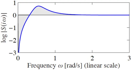
One notes, that this magnitude |S(jω)|<1 for all finite frequencies and can be made as small as desired by choosing a sufficiently large k.

Theorem 1. Bode’s integral formula. Assume that the loop transfer function L(s) of a feedback system goes to zero faster than ¹_s ass→ ∞, and let S(s) be the sensitivity function. If the loop transfer function has poles pk in the right-half-plane, then the sensitivity function satisfies the following integral:

Z ∞

0

log|S(jω)|dω = Z ∞

0

log 1

|1 +L(jω)|dω

=πX p_k.

(1.4)

This is usually called the principle of conservation of dirt.

What does this mean?

• Low sensitivity is desirable across a broad range of frequencies. It implies distur- bance rejection and good tracking.

Figure 1: Waterbed Effect.

• So much dirt we remove at some frequency, that much we need to add at some other frequency. This is also called the waterbed effect.

This can be resumed with Figure 1

Theorem 2. (Second waterbed formula) Suppose that L(s) has a single real RHP-zeroz or a complex conjugate pair of zeros z =x±jy and hasNp RHP-polespi. Let ¯pi denote the complex conjugate of ¯p_i. Then for closed-loop stability, the sensitivity function must satisfy

Z ∞

0

ln|S(jω)| ·w(z, ω)dω =π

N p

Y

I=1

|p_i +z

¯

p_i−z|, (1.5)

where

(w(z, ω) = _z2^2z+ω², if real zero

w(z, ω) = _x2+(y−ω)^{x 2} +_x2+(y+ω)^{x 2}, if complex zero. (1.6) Summarizing, unstable poles close to RHP-zeros make a plant difficult to control. These weighting functions make the argument of the integral negligible at ω > z. A RHP-zero reduces the frequency range where we can distribute dirt, which implies a higher peak for S(s) and hence disturbance amplification.

2 Digital Control

2.1 Signals and Systems

A whole course is dedicated to this topic (see Signals and Systems of professor D’Andrea).

A signal is a function of time that represents a physical quantity.

Continuous-timesignals are described by a functionx(t) such that this takes continuous values.

Discrete-timeSignals differ from continuous-time ones because of a sampling procedure.

Computers don’t understand the concept of continuous-time and therefore sample the signals, i.e. measure signal’s informations at specific time instants. Discrete-time are described by a function x[n] =x(n·T_s) where T_s is thesampling time. Thesampling frequency is defined as f_s = _T¹

s.

One can understand the difference between the two descriptions by looking at Figure 2.

t x(t)

Figure 2: Continuous-Time versus Discrete-Time representation

Advantages of Discrete-Time analysis

• Calculations are easier. Moreover, integrals become sums and differentiations be- come finite differences.

• One can implement complex algorithms.

Disadvantages of Discrete-Time analysis

• The sampling introduces a delay in the signal (≈e^−sTs2 )

• The informations between two samplings, that is betweenx[n] andx[n+ 1], are lost.

Every controller which is implemented on a microprocessor is a discrete-time system.

2.2 Discrete-Time Control Systems

Nowadays, controls systems are implemented in microcontrollers or in microprocessors in discrete-time and really rarely (see the lecture Elektrotechnik II) in continuous-time. As defined, although the processes are faster and easier, the informations are still sampled

and there is a certain loss of data. But how are we flexible about information loss? What is acceptable and what is not? The concept of aliasingwill help us understand that.

2.2.1 Aliasing

If the sampling frequency is chosed too low, i.e. one measures less times pro second, the signal can become poorly determined and the loss of information is too big to reconstruct it uniquely. This situation is called aliasing and one can find many examples of that in the real world. Let’s have a look to an easy example: you are finished with your summer’s exam session and you are flying to Ibiza, to finally enjoy the sun after a summer spent at ETH. You decide to film the turbine of the plane because, although you are on holiday, you have an engineer’s spirit. You land in Ibiza and, as you get into your hotel room, you want you have a look at your film. The rotation of the turbine’s blades you observe looks different to what it is supposed to be, and since you haven’t drunk yet, there must be some scientific reason. In fact, the sampling frequency of your phone camera is much lower than the turning frequency of the turbine: this results in a loss of information and hence in a wrong perception of what is going on.

Let’s have a more mathematical approach. Let’s assume a signal

x₁(t) = cos(ω·t). (2.1)

After discretization, the sampled signal reads

x₁[n] = cos(ω·T_s·n) = cos(Ω·n), Ω =ω·T_s. (2.2) Let’s assume a second signal

x₂(t) = cos

ω+2π T_s

·t

, (2.3)

where the frequency

ω₂ =ω+ 2π

T_s. (2.4)

is given. Using the periodicity of the cos function, the discretization of this second signal reads

x₂[n] = cos

ω+2π Ts

·T_s·n

= cos (ω·T_s·n+ 2π·n)

= cos(ω·Ts·n)

=x₁[n].

(2.5)

Although the two signals have different frequencies, they are equal when discretized. For this reason, one has to define an interval ofgood frequencies, where aliasing doesn’t occur.

In particular it holds

|ω|< π

T_s (2.6)

or

f < 1

2·T_s ⇔f_s >2·f_max. (2.7)

The maximal frequency accepted is f = _2·T¹

s and is called Nyquist frequency. In order to ensure good results, one uses in practice a factor of 10.

f < 1

10·T_s ⇔f_s >10·f_max. (2.8) For control systems the crossover frequency should be

f_s ≥10· ω_c

2π. (2.9)

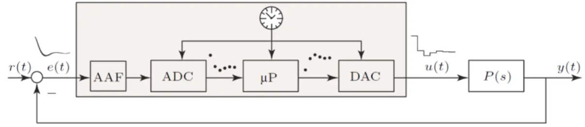
2.2.2 Discrete-time Control Loop Structure

The discrete-time control loop structure is depicted in Figure 3. This is composed of

Figure 3: Control Loop with AAF.

different elements, which we list in the following paragraphs.

Anti Aliasing Filter (AAF)

In order to solve this problem, an Anti Aliasing Filter (AAF) is used. The Anti Aliasing Filter is an analog filter and not a discrete one. In fact, we want to eliminate unwanted frequencies before sampling, because after that is too late (refer to Figure 3).

But how can one define unwanted frequencies? Those frequencies are normally the higher frequencies of a signal ¹. Because of that, as AAF one uses normally a low-pass filter.

This type of filter, lets low frequencies pass and blocks higher ones². The mathematic formulation of a first-order low-pass filter is given by

lp(s) = k

τ ·s+ 1. (2.10)

wherekis the gain andτ is the time constant of the system. The drawback of such a filter is problematic: the filter introduces additional unwanted phase that can lead to unstable behaviours.

Analog to Digital Converter (ADC)

At each discrete time step t =k·T the ADC converts a voltagee(t) to a digital number following a sampling frequency.

1Keep in mind: high signal frequency means problems by lower sampling frequency!

2This topic is exhaustively treated in the course Signals and Systems.

Microcontroller (µP)

This is a discrete-time controller that uses the sampled discrete-signal and gives back a dicrete output.

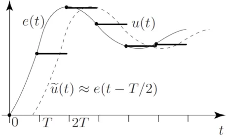
Digital to Analog Converter (DAC)

In order to convert back the signal, the DAC applies a zero-order-hold (ZOH). This introduces an extra delay of ^T₂ (refer to Figure 4).

Figure 4: Zero-Order-Hold.

2.3 Controller Discretization/Emulation

In order to understand this concept, we have to introduce the concept of z-transform.

2.3.1 The z-Transform

From the Laplace Transform to the z−transform

The Laplace transform is an integral transform which takes a function of a real variable t to a function of a complex variable s. Intuitively, for control systems t represents time and s represents frequency.

Definition 1. The one-sided Laplace transform of a signalx(t) is defined as L(x(t)) =X(s) = ˜x(s) =

Z ∞

0

x(t)e^−stdt. (2.11) Because of its definition, the Laplace transform is used to consider continuous-time sig- nals/systems. In order to deal with discrete-time system, one must derive its discrete analogon.

Example 2. Consider x(t) = cos(ωt). The Laplace transform of such a signal reads L(cos(ωt)) =

Z ∞

0

e^−stcos(ωt)dt

=−1

se^−stcos(ωt)

∞ 0

− ω s

Z ∞

0

e^−stsin(ωt)dt

= 1 s − ω

s

−1

se^−stsin(ωt)

∞ 0

+ω s

Z ∞

0

e^−stcos(ωt)dt

= 1 s − ω²

s²L(cos(ωt)).

(2.12)

From this equation, one has

L(cos(ωt)) = s

s²+ω² (2.13)

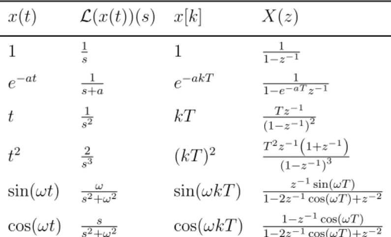
Some of the known Laplace transforms are listed in Table 1.

Laplace transforms receive as inputs functions, which are defined in continuous-time. In order to analyze discrete-time system, one must derive its discrete analogue. Discrete time signals x(kT) = x[k] are obtained by sampling a continuous-time function x(t). A sample of a function is its ordinate at a specific time, called the sampling instant, i.e.

x[k] =x(tk), tk =t0+kT, (2.14) where T is the sampling period. A sampled function can be expressed through the mul- tiplication of a continuous funtion and a Dirac comb (see reference), i.e.

x[k] =x(t)·D(t), (2.15)

with D(t) which is a Dirac comb.

Definition 2. A Dirac comb, also known as sampling function, is a periodic distribution constructed from Dirac delta functions and reads

D(t) =

∞

X

k=−∞

δ(t−kT). (2.16)

Remark. An intuitive explanation of this, is that this function is 1 for t=kT and 0 for all other cases. Since k is a natural number, i.e. k =−∞, . . . ,∞, applying this function to a continuous-time signal consists in considering informations of that signal spaced with the sampling time T.

Imagine to have a continuous-time signal x(t) and to sample it with a sampling periodT. The sampled signal can be described with the help of a Dirac comb as

xm(t) =x(t)·

∞

X

k=−∞

δ(t−kT)

=

∞

X

k=−∞

x(kT)·δ(t−kT)

=

∞

X

k=−∞

x[k]·δ(t−kT),

(2.17)

where we denote x[k] as the k−th sample of x(t). Let’s compute the Laplace transform of the sampled signal:

X_m(s) = L(x_m(t))

(a) =

Z ∞

0

xm(t)e^−stdt

= Z ∞

0

∞

X

k=−∞

x[k]·δ(t−kT)e^−stdt

(b) =

∞

X

k=−∞

x[k]· Z ∞

0

δ(t−kT)e^−stdt

(c) =

∞

X

k=−∞

x[k]e^−ksT,

(2.18)

where we used

(a) This is an application of Definition 1.

(b) The sum and the integral can be switched because the functionf(t) =δ(t−kT)e^−st is non-negative. This is a direct consequence of the Fubini/Tonelli’s theorem. If you are interested in this, have a look at https://en.wikipedia.org/wiki/Fubini%

27s_theorem.

(c) This result is obtained by applying the Dirac integral property, i.e.

Z ∞

0

δ(t−kT)e^−stdt=e^−ksT. (2.19)

By introducing the variable z =e^sT, one can rewrite Equation 2.18 as X_m(z) =

∞

X

k=−∞

x[k]z^−k, (2.20)

which is defined as the z−transform of a discrete time system. We have now found the relation between the z transform and the Laplace transform and are able to apply the concept to any discrete-time signal.

Definition 3. The bilateral z−transform of a discrete-time signal x[k] is defined as X(z) =Z((x[k]) =

∞

X

k=−∞

x[k]z^−k. (2.21)

Some of the known z−transforms are listed in Table 1.

Properties

In the following we list some of the most important properties of the z−transform. Let X(z), Y(z) be thez−transforms of the signals x[k], y[k].

x(t) L(x(t))(s) x[k] X(z)

1 ¹_s 1 _1−z¹−1

e^−at _s+a¹ e^−akT _1−e−aT¹ z⁻¹

t _s¹2 kT _(1−z^{T z−1}₋₁

)²

t² _s²3 (kT)^{2 T}

2z⁻¹(^1+z−1)

(1−z⁻¹)³

sin(ωt) _s2+ω^{ω 2} sin(ωkT) _1−2z^z−1⁻¹cos(ωT)+z^{sin(ωT) −2}

cos(ωt) _s2+ω^{s 2} cos(ωkT) _1−2z^1−z−1⁻¹cos(ωT)+z^cos(ωT)−2

Table 1: Known Laplace andz−transforms.

1. Linearity

Z(ax[k] +by[k]) = aX(z) +bY(z). (2.22) Proof. It holds

Z(ax[k] +by[k]) =

∞

X

k=−∞

(ax[k] +by[k])z^−k

=

∞

X

k=−∞

ax[k]z^−k+

∞

X

k=−∞

by[k]z^−k

=aX(z) +bY(z).

(2.23)

2. Time shifting

Z(x[k−k₀]) = z^−k0X(z). (2.24) Proof. It holds

Z(x[k−k₀]) =

∞

X

k=−∞

x[k−k₀]z^−k. (2.25) Define m=k−k₀. It holds k =m+k₀ and

∞

X

k=−∞

x[k−k₀]z^−k=

∞

X

k=−∞

x[m]z^−mz^−k0

=z^−k0X(z).

(2.26)

3. Convolution ∗

Z(x[k]∗y[k]) =X(z)Y(z). (2.27)

Proof. Follows directly from the definition of convolution.

4. Reverse time

Z(x[−k]) = X 1

z

. (2.28)

Proof. It holds

Z(x[−k]) =

∞

X

k=−∞

x[−k]z^−k

=

∞

X

r=−∞

x[r]

1 z

−r

=X 1

z

.

(2.29)

5. Scaling in z domain

Z a^kx[k]

=Xz a

. (2.30)

Proof. It holds

Z a^kx[k]

=

∞

X

k=−∞

x[k]z a

^−k

=X z

a

.

(2.31)

6. Conjugation

Z(x^∗[k]) =X^∗(z^∗). (2.32)

Proof. It holds

X^∗(z) =

∞

X

k=−∞

x[k]z^−k

!∗

=

∞

X

k=−∞

x^∗[k](z^∗)^−k.

(2.33)

Replacing z by z^∗ one gets the desired result.

7. Differentiation in z domain

Z(kx[k]) = −z ∂

∂zX(z). (2.34)

Proof. It holds

∂

∂zX(z) = ∂

∂z

∞

X

k=−∞

x[k]z^−k

linearity of sum/derivative =

∞

X

k=−∞

x[k] ∂

∂zz^−k

=

∞

X

k=−∞

x[k](−k)z^−k−1

=−1 z

∞

X

k=−∞

kx[k]z^−k,

(2.35)

from which the statement follows.

Approximations

In order to use this concept, often the exact solution is too complicated to compute and not needed for an acceptable result. In practice, approximations are used. Instead of considering the derivative as it is defined, one tries to approximate this via differences.

Given y(t) = ˙x(t), the three most used approximation methods are

• Euler forward:

y[k]≈ x[k+ 1]−x[k]

T_s (2.36)

• Euler backward:

y[k]≈ x[k]−x[k−1]

T_s (2.37)

• Tustin method

y[k]−y[k−1]

2 ≈ x[k]−x[k−1]

T_s (2.38)

The meaning of the variable z can change with respect to the chosen discretization ap- proach. Here, just discretization results are presented. You can try derive the following rules on your own. A list of the most used transformations is reported in Table 2. The

Exact s = 1 Ts

·ln(z) z =e^s·Ts Euler forward s = z−1

T_s z =s·T_s+ 1 Euler backward s = z−1

z·T_s z = 1 1−s·T_s Tustin s = 2

T_s · z−1

z+ 1 z = 1 +s· ^T₂^s 1−s· ^T₂^s Table 2: Discretization methods and substitution.

different approaches are results of different Taylor’s approximations³:

3As reminder: e^x≈1 +x.

• Forward Euler:

z =e^s·Ts ≈1 +s·T_s. (2.39)

• Backward Euler:

z =e^s·Ts = 1

e^−s·Ts ≈ 1 1−s·Ts

. (2.40)

• Tustin:

z= e^s·Ts2

e^−s·Ts2 ≈ 1 +s·^T₂^s

1−s·^T₂^s. (2.41)

In practice, the most used approach is the Tustin transformation, but there are cases where the other transformations could be useful.

Example 3. You are given the differential relation y(t) = d

dtx(t), x(0) = 0. (2.42)

One can rewrite the relation in the frequency domain using the Laplace transform. Using the property for derivatives

L d

dtf(t)

=sL(f(t))−f(0). (2.43)

By Laplace transforming both sides of the relation and using the given initial condition, one gets

Y(s) = sX(s). (2.44)

In order to discretize the relation, we sample with a generic sampling time T the signals.

Forward Euler’s method for the approximation of differentials reads

˙

x(kT)≈ x((k+ 1)T)−x(kT)

T . (2.45)

The discretized relation reads

y(kT) = x((k+ 1)T)−x(kT)

T . (2.46)

In order to compute thez-transform of the relation, one needs to use its time shift property, i.e.

Z(x((k−k₀)T)) =z^−k0Z(x(kT)). (2.47) In this case, the shift is of -1 and transforming both sides of the relation results in

Y(z) = zX(z)−X(z)

T = z−1

T X(z). (2.48)

By using the relations of Equation (2.44) and Equation (2.48), one can write s = z−1

T . (2.49)

2.4 State Space Discretization

Starting from the continuous-time state space form

˙

x(t) = Ax(t) +Bu(t)

y(t) = Cx(t) +Du(t), (2.50)

one wants to obtain the discrete-time state space representation x[k+ 1] =A_dx[k] +B_du[k]

y[k] =Cdx[k] +Ddu[k]. (2.51) By recalling that x[k + 1] = x((k + 1)T), one can start from the solution derived for continuous-time systems

x(t) = e^Atx(0) +e^At Z t

0

e^−AτBu(τ)dτ. (2.52)

By plugging into this equation t= (k+ 1)T, one gets x((k+ 1)T) =e^A(k+1)Tx(0) +e^A(k+1)T

Z (k+1)T

0

e^−AτBu(τ)dτ (2.53) and hence

x(kT) =e^AkTx(0) +e^AkT Z kT

0

e^−AτBu(τ)dτ. (2.54) Since we want to write x((k+ 1)T) in terms ofx(kT), we multiply all terms of Equation (2.54) by e^AT and rearrange the equation as

e^A(k+1)Tx(0) =e^ATx(kT)−e^A(k+1)T Z kT

0

e^−AτBu(τ)dτ. (2.55) Substituting this result into Equation (2.53), one gets

x((k+ 1)T) =e^ATx(kT)−e^A(k+1)T Z kT

0

e^−AτBu(τ)dτ+e^A(k+1)T

Z (k+1)T

0

e^−AτBu(τ)dτ

=e^ATx(kT) +e^A(k+1)T

Z (k+1)T

kT

e^−AτBu(τ)dτ

=e^ATx(kT) +

Z (k+1)T

kT

e^{A[(k+1)T−τ]}Bu(τ)dτ (a) =e^ATx(kT)−

Z 0

T

e^AαBdαu(kT).

= e^AT

|{z}

Ad

x[k] + Z T

0

e^AαBdα

| {z }

Bd

u[k],

(2.56) where we used

(a) α= (k+ 1)T −τ, dα =−dτ.

It follows that

Ad =e^AT, B_d =

Z T

0

e^AαBdα, C_d =C,

D_d =D.

(2.57)

Example 4. Given the general state space for in Equation (2.50) The forward Euler approach for differentials reads

˙

x≈ x[k+ 1]−x[k]

T_s . (2.58)

Applying this to the generic state space formulation

˙

x(t) = Ax(t) +Bu(t)

y(t) = Cx(t) +Du(t), (2.59)

one gets

x[k]−x[k−1]

T_s =Ax[k] +Bu[k]

y[k] =Cx[k] +Du[k],

(2.60)

which results in

x[k+ 1] = (I+TsA)

| {z }

A_d,f

x[k] +TsB

|{z}

Bd,f

u[k]

y[k] = C

|{z}

Cd,f

x[k] + D

|{z}

Dd,f

u[k]. (2.61)

Example 5. You are given the system

˙ x(t) =

1 −1

2 4

x(t) +

1 0

u(t) y(t) = 1 1

x(t).

(2.62)

(a) Find the discrete-time state space representation of the system using a sampling time T_s = 1s, i.e. find A_d, B_d, C_d, D_d

Solution. In order to compute the exact discretization, we use the formulas derived in class. For A_d, one has

A_d =e^ATs =e^A. (2.63)

In order to compute the matrix exponential, one has to compute its eigenvalues, store them in a matrix D, find its eigenvectors, store them in matrixT, find the diagonal form and use the law

e^A=T e^DT⁻¹. (2.64)

First, we compute the eigenvalues of A. It holds P_A(λ) = det(A−λI)

= det

1−λ −1 2 4−λ

=λ²−5λ+ 6

= (λ−2)·(λ−3).

(2.65)

Therefore, the eigenvalues are λ₁ = 2 and λ₂ = 3 and they have algebraic multiplicity 1.

We compute now the eigenvectors:

• E_λ1 =E₂: from (A−λ₁I)x= 0 one gets the system of equations −1 −1 0

2 2 0

One can note that the second row is linear dependent with the first. We therefore have a free parameter and the eigenspace for λ₁ reads

E₂ =n

−1 1

o

. (2.66)

E₂ has geometric multiplicity 1.

• E_λ2 =E₃: from (A−λ₂I)x= 0 one gets the system of equations −2 −1 0

2 1 0

One notes that the first and the second row are linearly dependent. We therefore have a free parameter and the eigenspace for λ₂ reads

E₃ =n

−1 2

o

(2.67) E₃ has geometric multiplicity 1. Since the algebraic and geometric multiplicity concide for every eigenvalue of A, the matrix is diagonalizable. With the computed eigenspaces, one can build the matrix T as

T =

−1 −1

1 2

, (2.68)

and D as a diagonal matrix with the eigenvalues on the diagonal:

D= 2 0

0 3

. (2.69)

It holds

T⁻¹ = 1 (−2 + 1)·

2 1

−1 −1

=

−2 −1

1 1

.

(2.70)

Using Equation (2.64) one gets A_d=e^A

=T e^DT⁻¹

=

−1 −1

1 2

·

e² 0 0 e³

·

−2 −1

1 1

=

2e² −e³ e²−e³

−2e²+ 2e³ −e²+ 2e³

.

(2.71)

For B_d holds

B_d = Z Ts

0

e^AτBdτ

= Z 1

0

e^AτBdτ

= Z 1

0

−1 −1

1 2

·

e^2τ 0 0 e^3τ

·

−2 −1

1 1

· 1

0

dτ

= Z 1

0

−e^2τ −e^3τ e^2τ 2e^3τ

· −2

1

dτ

= Z 1

0

2e^2τ−e^3τ

−2e^2τ + 2e^3τ

dτ

=

e²−^e₃³ − ²₃

−e²+ ²₃e³+ ¹₃

.

(2.72)

Furthermore, one has C_d =C and D_d =D= 0.

References

[1] Analysis III notes, ETH Zurich.

[2] Karl Johan Amstroem, Richard M. Murray Feedback Systems for Scientists and En- gineers. Princeton University Press, Princeton and Oxford, 2009.

[3] Sigurd Skogestad, Multivariate Feedback Control. John Wiley and Sons, New York, 2001.

[4] https://en.wikipedia.org/wiki/Dirac_comb

[5] https://ccrma.stanford.edu/~jos/Laplace/Laplace_4up.pdf